A constrained edit distance algorithm between semi-ordered trees

(1)

A constrained edit distance algorithm between semi-ordered trees

Aïda Ouangraoua

∗

, Pascal Ferraro

LaBRI - Université de Bordeaux 1, 351 Cours de la Libération, 33405 Talence Cedex, France

a r t i c l e i n f o

Article history:

Received 19 February 2008

Received in revised form 17 September 2008 Accepted 17 November 2008 Communicated by M. Crochemore Keywords: Semi-ordered trees Theory of computation Tree editing Dynamic programming a b s t r a c t

In this paper, we propose a formal definition of a new class of trees calledsemi-ordered trees

and a polynomial dynamic programming algorithm to compute a constrained edit distance between such trees. The core of the method relies on a similar approach to compare unordered [Kaizhong Zhang, A constrained edit distance between unordered labeled trees, Algorithmica 15 (1996) 205–222] and ordered trees [Kaizhong Zhang, Algorithms for the constrained editing distance between ordered labeled trees and related problems, Pattern Recognition 28 (3) (1995) 463–474]. The method is currently applied to evaluate the similarity between architectures of apple trees [Vincent Segura, Aida Ouangraoua, Pascal Ferraro, Evelyne Costes, Comparison of tree architecture using tree edit distances: Application to two-year-old apple tree, Euphytica 161 (2007) 155–164].

Edit distances, initially introduced for string-to-string comparison [1], were later extended to compare ordered trees [2,

3] and unordered trees [4]. Ordered trees are trees in which the left-to-right order of each node’s children is fixed [2] while unordered trees are trees in which no order is considered on the set of children of any vertex.

In this context, the tree-to-tree edition problem consists in determining a sequence of edit operations (substitutions, insertions and deletions of vertices) of minimum cost needed to transform one tree into the other, the cost of a sequence being the sum of the costs of its edit operations. The edit operations are constrained in order to preserve the topology of trees after their application. Basically, in an optimal sequence of edit operations no more than one edit operation can be applied on any vertex of a tree and the edit operations must maintain the ancestor–descendant relation between vertices. Furthermore, in ordered tree comparisons, an additional constraint is added to maintain the left-to-right order of each node’s children [2] while in the case of unordered trees an additional constraint preserves the descendants of the nearest common ancestor of two vertices [4].

In this paper, we propose unifying these two approaches by introducing a new class of trees calledsemi-ordered trees. Asemi-ordered treeis a tree with a semi-order relation defined on the set of children of each vertex. Thus, ordered and unordered trees can be considered as semi-ordered trees using an appropriate definition of the semi-order relations between children of vertices. Finally, we propose an algorithm to compute a constrained edit distance between two semi-ordered trees using the dynamic programming principle.

The introduction ofsemi-ordered treesis motivated by a biological application. Indeed, in most botanical applications, trees are used to represent the topological structure of plant architectures [5] and then to evaluate the similarity between these architectures using edit distances [6]. Generally, the topological structure of plant architectures can be modeled by ordered trees. However, the order between the components of a plant is often partially measured and in some cases, only semi-order relations instead of order relations are measured between the components. In these cases, plant architectures can be modeled by semi-ordered trees.

∗_{Corresponding author. Tel.: +33 5 40 00 35 10.}

(2)

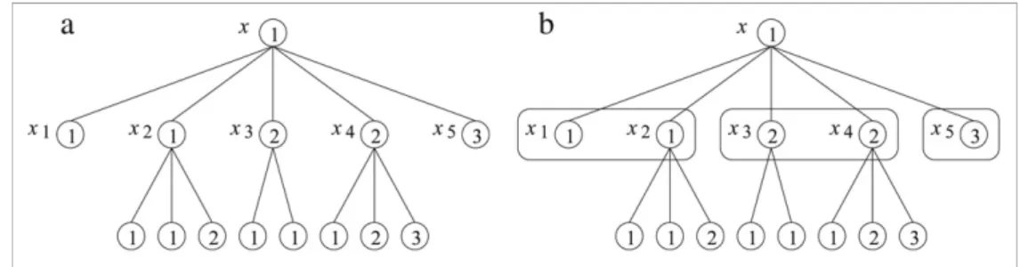
Fig. 1.(a) A semi-ordered treeT, (b) the ordered partition of the children of the vertexxinduced by the total semi-order relationvxon C(x). In Section2, we formally define a semi-ordered tree. In Section3, we first define the notion ofmapping between two semi-ordered trees, and then a polynomial algorithm for the computation of a constrained edit distance between semi-ordered trees is described.

2. Semi-ordered trees

A directed graphG

=

(

V

,

E

)

consists of a setVof vertices, a setEof edges, each edge being represented by an ordered pair of vertices. The order (i.e. number of vertices) of a graphG

=

(

V

,

E

)

is denoted by

|G|

and the number of vertices in a subset of verticesX

⊆

Vis denoted by

|X|

. IfGis a directed graph then for any edge

(

x

,

y

)

inE,xandyare called aparent-child pair. Arooted treeis then an acyclic, connected, directed graphT

=

(

V

,

E

)

in which every vertex except one (the rootr) has exactly one parent vertex: the root has no parent. Theparentof a vertexxis denoted by P

(

x

)

and the set ofchildrenof xis denoted by C

(

x

)

. A path between two verticesxandyis a (possibly empty) sequence of edges

{

(

xi

,

xi+1

)

i=1,n

}

such that

x1

=

xandxn+1

=

y. A vertexyis then adescendantof a vertexx(and reciprocallyxis anancestorofy) if there exists a path betweenxandy. The ancestor–descendant relation on the set of vertices of a rooted tree is a partial order relation on the set of its vertices denoted by

≤

: byx

≤

ywe mean thatxis an ancestor ofy. Thenearest common ancestorof two verticesx andyofT, denoted byx

∧

y, is the common ancestor ofxandysuch that for any common ancestorzofxandy,z

≤

(

x

∧

y

)

. In the following,T

[x]

denotes the subtree ofTrooted atxwhich contains all the descendants ofx, and the empty tree and the empty graph are both denoted by

∅ =

(

∅

,

∅

)

.

Aforestis a set of rooted trees. The set of the roots of the trees composing a forestFis denoted by roots

(

F

)

. LetT be a rooted tree. Letxbe a vertex ofT. LetX

= {x

1

, . . . ,

xn

}

be a subset of C

(

x

)

.F[X]denotes the subforest ofT consisting of subtrees rooted at vertices ofX,F[X] = {T

[x

1

]

, . . . ,

T

[x

n

]}

. Thus, the subforest of a vertexxdenoted byF

[

C

(

x

)

]

is obtained fromT

[x]

by removing the rootxand all edges incident withx.F[C

(

x

)

]

is simply denoted byF[x].

An ordered tree is a pair

(

T

,

S

)

whereTis a rooted tree andS

= {

x

,

x

∈

T

}

is a set of total order relations such that for any vertexxofT,

_xis a total order relation on C

(

x

)

. The set of total order relationsSand the ancestor–descendant relation

≤

on the vertices ofTinduce two total order relations on the set of vertices ofT(namelyprefixorpostfixorder relations). An unordered tree is a rooted treeTsuch that the only significant relation between the vertices ofTis the ancestor–descendant relation (all the children of a vertex ofTare equivalent). We propose unifying these two classes of trees in a single one called semi-ordered trees (Fig. 1.a). Asemi-order relation[7]

v

on a setVis a reflexive and transitive binary relation onV.

v

is a total semi-order relationif for any pair

(

x

,

y

)

of elements ofV,x

v

yory

v

x, otherwise

v

is calledpartial semi-order relation. InFig. 1, the total semi-order relation on the set of children of a given vertex in a tree is defined by the relation ‘‘less than or equal to’’ on the numbers associated to the vertices.

Definition 1 (Semi-ordered Tree). A semi-ordered tree is a pair

(

T

,

Sv

)

whereTis a rooted tree andSv

= {v

x

,

x

∈

T

}

is a set of total semi-order relations such that for any vertexxofT,

v

_xis a total semi-order relation on C

(

x

)

.

Note that an unordered treeTis a semi-ordered tree

(

T

,

Sv

)

such that for any vertexxofT,

v

xis an equivalence relation having only one equivalence class,i.e.for any pair

(

x1

,

x2

)

in C

(

x

)

×

C

(

x

)

,x1

v

x x2andx2

v

x x1(all the children ofxare equivalent). Similarly, an ordered treeT is a semi-ordered tree

(

T

,

Sv

)

such that for any vertexxofT,

v

xis a total order relation on C

(

x

)

. A semi-order (or pre-order) relation on C

(

x

)

means that some elements of C

(

x

)

are equivalent (equal) while some others can be totally ordered. If there are some elements which are not comparable then the semi-order is partial otherwise it is a total semi-order relation.

Let

(

T

,

Sv

)

be a semi-ordered tree. The set of semi-order relationsSvand the ancestor–descendant relation

≤

on the

vertices ofTinduce an order relation denoted by

v

on the set of vertices ofTdefined as follows. Let us consider two vertices xandy.xwill be smaller thanyaccording to

v

if and only ifxis an ancestor ofyor there exists two ancestorsandtof respectivelyxandy, having the same parentusuch thatsis strictly smaller thantaccording to

v

_u.

Formally, for any vertexuofT ands

,

t

∈

C

(

u

)

, the relations

v

_u tandt

6v

_usis denoted bys@ut. The order relation

v

is such that for any pair

(

x

,

y

)

of vertices ofT,xandysatisfyx

v

yif and only ifxis an ancestor ofyor there is a pair

(

s

,

t

)

of vertices in C

(

x

∧

y

)

such thats

≤

xandt

≤

yands@x∧yt:

∀x

,

y

∈

V

,

x

v

y

⇔

x

≤

yor

,

(3)

elements ofV(defining a partition ofV) is denoted byV≡

= {[x] |

x

∈

V}. In the same way, the total semi-order relation

v

induces atotal order relation

(i.e.reflexive, transitive and antisymmetric) onV≡defined by:

∀[x]

,

[y] ∈

V≡

,

[x] [y] ⇔

x

v

y

.

For any vertexxofT, thepartitionof C

(

x

)

induced by

v

_x is denoted by C

(

x

)

≡(Fig. 1.b). For any setXin C

(

x

)

≡, the left-classofXdenoted byX−_{is the set of all vertices}_x

iin C

(

x

)

such that for any vertexxjinX,xi @xjand the

augmented-left-classofXdenoted byX+is defined asX+

=

X

∪

X−. The maximal setXof C

(

x

)

≡for the order relation defined on

C

(

x

)

≡is such that C

(

x

)

=

X+, then the subforest ofxis the subforest ofT consisting of subtrees rooted at vertices ofX+, F[x] =F

[X

+

_]

_.

For example, in Fig. 1.b, the ordered partition of C

(

x

)

is C

(

x

)

≡

=

{{x

1

,

x2

}

,

{x

3

,

x4

}

,

{x

5

}}

. If the set X is

{x

1

,

x2

}

(respectively,

{x

3

,

x4

}

;

{x

5

}

) then the left-class ofXisX−

= ∅

(respectively,X−

= {x

1

,

x2

}

;X−

= {x

1

,

x2

,

x3

,

x4

}

) and the augmented-left-class ofXisX+

_{= {x}

1

,

x2

}

(respectively,X+

= {x

1

,

x2

,

x3

,

x4

}

;X+

=

C

(

x

)

).

Asemi-ordered forestis a pair

(

F

,

v

_F

)

whereFis a set of semi-ordered trees and

v

_F is a total semi-order relation on roots

(

F

)

. Note that, for any setXin C

(

x

)

≡,

(

F[X]

,

v

x

)

,

(

F

[X

−

]

,

v

x

)

and

(

F

[X

+

]

,

v

x

)

are semi-ordered forests sinceF

[X]

,

F[X−

]

andF

[X

+

]

are sets of semi-ordered trees and

v

_xis a total semi-order relation on roots

(

F

[X]

)

=

X, roots

(

F[X−

]

)

=

X− and roots

(

F[X+

_]

₎

₌

_X+_.

In the following, trees are labeled on an alphabetΣand

α

is a function that associates a label ofΣto each vertex of a tree T

=

(

V

,

E

)

,

α

:

V

→

Σ. A distancedis assumed to be defined on the labels ofΣ. A distance1_{between vertices is defined} usingd:

γ (

x

,

y

)

=

d

(α(

x

), α(

y

))

. Let

λ

be a symbol not inΣ.dis extended by defining quantitiesd

(α(

x

), λ)

andd

(λ, α(

y

))

such thatdis a distance onΣ

∪ {

λ

}

. The distanced

(α(

x

), λ)

between the label of a vertexxand the label

λ

is denoted by

γ (

x

, λ)

by convention, and similarly for

γ (λ,

y

)

.

In the following,

(

T1

,

Sv1

)

and

(

T2

,

Sv2

)

are two semi-ordered trees. If there is no confusion,

(

T1

,

Sv1

)

and

(

T2

,

Sv2

)

are respectively denoted byT1andT2,

v

1and

v

2are the partial order relations respectively defined on the set of vertices ofT1 andT2. They are simply denoted by

v

if there is no confusion.

3. Edit distance

The computation of an edit distance between two trees consists in determining a sequence of edit operations of minimum cost which transforms an initial tree into a target tree. In order to characterize the effect of a sequence of edit operations between two trees, edit distance mappings between vertices of trees has been introduced in [4] for unordered and [2,3] for ordered trees.

3.1. Mapping between semi-ordered trees

An optimal sequence of edit operations (i.e. a sequence having a minimum cost) from T1 to T2 is such that the corresponding mapping associates a vertex ofT1to at most one vertex ofT2and reciprocally and preserves the relations defined on the vertices ofT1andT2, namely the ancestor–descendant relation and the semi-order relations. The preservation of the ancestor–descendant relationship

≤

and the semi-order relations

v

_xis equivalent to the preservation of

≤

and the order relation

v

induced on the vertices ofT1andT2.

Avalid mappingfromT1

=

(

V1

,

E1

)

toT2

=

(

V2

,

E2

)

is a setMof ordered pairs of vertices

(

s

,

s0

)

withs

∈

V1ands0

∈

V2 such that for any pairs

(

s

,

s0

₎

_and

₍

_t

_,

_t0

₎

_in_M_:

s

=

t

⇔

s0

=

t0

(

one-to-one

)

s

≤

t

⇔

s0

≤

t0

(

ancestor–descendant preservation

)

s

v

t

⇔

s0

v

t0

(

semi-order preservation

)

For any pair

(

s

,

s0

)

inM,sands0are called images of each other and are denoted byM

(

s

)

=

s0andM

(

s0

)

=

s. If there is no confusion,

(

s

,

s0

₎

_∈

_M_{is denoted by}_s

_∈

_M_and_s0

_∈

_M_{. Let}_F

1(respectively,F2) be a subforest ofT1(respectively,T2). The

1 A distancedon a setVis a function that associates to each pair of elements ofVa non-negative real such that for anyx,y,zinV,d(x,y)=0 if and only ifx=y,d(x,y)=d(y,x)andd(x,y)+d(y,z)≥d(x,z).

(4)

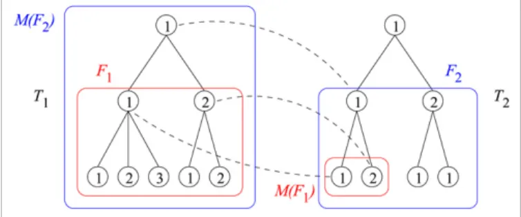
Fig. 2.A valid mapping from a semi-ordered treeT1to a semi-ordered treeT2and the imagesM(F1)andM(F2)of subforestsF1andF2ofT1andT2

respectively. The vertices ofT1andT2images of each other are linked by dotted lines.

Fig. 3.Examples of mappings between two semi-ordered treesT1andT2.M= {(x,y), (w1, w2), (x1,x2), (y1,y2), (z1,z2)}is a not valid mapping fromT1

toT2:y1vz1whereasy26vz2.M\{(z1,z2)}is a valid but not constrained mapping:(w1∧x1)≤y1whereas(w2∧x2)6≤y2.M\{(y1,y2), (z1,z2)}is a

constrained mapping fromT1toT2.

image ofF₁(respectively,F₂) denoted byM

(

F₁

)

(respectively,M

(

F₂

)

) is the subforest ofT₂(respectively,T₁) containing all the images of vertices ofF1(respectively,F2) and their descendants. The concept of mapping is extended to forests and sets of vertices not necessarily connected.

LetMbe a valid mapping fromT1toT2(Fig. 2). LetI(respectively,J) be the set of vertices ofT1(respectively,T2) which do not appear in a pair ofM. The cost ofMis defined by:

γ (

M

)

=

X

(s,s0₎_∈_M

γ (

s

,

s0

)

+

X

s∈I

γ (

s

, λ)

+

X

s0_∈_J

γ (λ,

s0

).

Theedit distancebetweenT1andT2is the minimum cost of a valid mapping fromT1toT2. Since unordered trees are particular cases of semi-ordered trees, computing the edit distance between two semi-ordered trees is at least as hard as the computation of the edit distance between unordered trees which is a MAX-SNP-hard problem [8].

3.2. Constrained edit distance

Since the computation of the edit distance between two semi-ordered trees is a MAX-SNP-hard problem, we consider a constrained version of the problem: the computation on semi-ordered trees of theconstrained edit distanceintroduced by Zhang [4] to compare unordered trees.

Aconstrained mappingfromT1toT2is a valid mapping

(

M

,

T1

,

T2

)

such that for any pairs

(

s

,

s0

)

,

(

t

,

t0

)

and

(

u

,

u0

)

inM:

(

s

∧

t

)

≤

u

⇔

(

s0

∧

t0

)

≤

u0

(

structure preservation

)

Examples of mappings between semi-ordered trees are presented inFig. 3. Let x(respectively,y) be a vertex ofT1 (respectively,T2). LetX

= {x

1

, . . . ,

xn

}

(respectively,Y

= {y

1

, . . . ,

ym

}

) be a subset of C

(

x

)

(respectively, C

(

y

)

). The set of constrained mappings fromT1

[x]

toT2

[y]

(respectively,F1

[X]

toF2

[Y

]

) is denoted byMC

(

T1

[x]

,

T2

[y]

)

(respectively, MC

(

F1

[X]

,

F2

[Y

]

)

).

Definition 2 (Constrained Edit Distance). The constrained edit distance between T1 and T2 is the minimum cost of a constrained mapping fromT1toT2:

DC

(

T1

,

T2

)

=

min

{

γ (

M

)

|

M

∈

MC

(

T1

,

T2

)

}

.

Zhang [4] has described a dynamic programming algorithm to compute the constrained edit distance between two

unordered trees using reductions of some subproblems tominimum cost maximum flow problems[9]. Similarly, we propose in the following a reduction of the computation of the constrained edit distance between semi-ordered trees to minimum cost maximum flow problems. The following recurrence formulas form the basis of the algorithm for the computation of the constrained edit distance between two semi-ordered trees.

(5)

Fig. 4.A restricted mapping fromF1[C(x)]toF2[C(y)]such thatP(M)= {(x1,y1), (x2,y3)}.

Lemma 3 (Initialization). Let x, y be two vertices of T1and T2respectively. X and Y are two sets of vertices respectively in C

(

x

)

≡ and C

(

y

)

≡:











DC

(

∅

,

∅

)

=

0 DC

(

T1

[x]

,

∅

)

=

γ (

x

, λ)

+

DC

(

F1

[x]

,

∅

)

DC

(

F1

[X]

,

∅

)

=

P

xk∈XDC

(

T1

[x

k

]

,

∅

)

DC

(

F1

[X

+

]

,

∅

)

=

DC

(

F1

[X]

,

∅

)

+

DC

(

F1

[X

−

]

,

∅

)

DC

(

∅

,

T2

[

y

]

)

=

γ (λ,

y

)

+

DC

(

∅

,

F2

[

y

]

)

DC

(

∅

,

F2

[Y

]

)

=

P

yk∈YDC

(

∅

,

T2

[y

k

]

)

DC

(

∅

,

F2

[Y

+

]

)

=

DC

(

∅

,

F2

[Y

]

)

+

DC

(

∅

,

F2

[Y

−

]

).

Proof. The two first formulas are obvious. Since the forestF1

[X]

is composed of subtrees rooted at vertices ofX,DC

(

F1

[X]

,

∅

)

is equal to the sum of the valuesDC

(

T1

[x

k

]

,

∅

)

such thatxkis a vertex inX. SinceX+

=

X

∪

X−,DC

(

F1

[X

+

]

,

∅

)

is equal to DC

(

F1

[X]

,

∅

)

plusDC

(

F1

[X

−

]

,

∅

)

. The proofs of the last three formulas are symmetric to the previous proofs.

Lemma 4 (Constrained Edit Distance Between Subtrees). Let x and y be two vertices of T1and T2respectively. The constrained edit distance between T1

[x]

and T2

[y]

is:

DC

(

T1

[x]

,

T2

[y]

)

=

min

(

_D

C

(

F1

[x]

,

F2

[y]

)

+

γ (

x

,

y

)

minyk∈C(y)

{D

C

(

T1

[x]

,

T2

[y

k

]

)

−

DC

(

∅

,

T2

[y

k

]

)

} +

DC

(

∅

,

T2

[y]

)

minxk∈C(x)

{D

C

(

T1

[x

k

]

,

T2

[y]

)

−

DC

(

T1

[x

k

]

,

∅

)

} +

DC

(

T1

[x]

,

∅

).

The proof ofLemma 4(inAppendix) is similar to the proof of Lemma 6 in [4]. Indeed, only the preservation of ancestor– descendant relations is needed to computeDC

(

T1

[x]

,

T2

[y]

)

.

However, to computeDC

(

T1

[x]

,

T2

[y]

)

, we first need to computeDC

(

F1

[x]

,

F2

[y]

)

. The computation ofDC

(

F1

[x]

,

F2

[y]

)

uses the notion ofrestricted mappingintroduced by Zhang [4] using a different formalism. LetX

= {x

1

, . . . ,

xn

}

(respectively,

Y

= {y

1

, . . . ,

ym

}

) be a subset of C

(

x

)

(respectively, C

(

y

)

). Arestricted mappingfromF1

[X]

toF2

[Y

]

is a constrained mapping MfromF1

[X]

toF2

[Y]

)

such that for any pairs

(

s

,

s0

)

and

(

t

,

t0

)

inM(Fig. 4):

(

s

∧

t

)

∈

F1

[

X

] ⇔

(

s

0

_∧

t0

)

∈

F2

[

Y

]

This means that each tree ofF1

[X]

is mapped on at most one tree ofF2

[Y]

and reciprocally. Thus,M induces a valid mapping fromXtoYdenoted byP

(

M

)

(Fig. 4) and defined as follows:

P

(

M

)

= {

(

xi

,

yj

)

∈

X

×

Y

|

M

(

T1

[x

i

]

)

⊆

M

(

T2

[y

j

]

)

and M

(

T2

[y

j

]

)

⊆

M

(

T1

[x

i

]

)

}

.

The set of restricted mappings fromF1

[X]

toF2

[Y

]

is denoted byR

(

F1

[X]

,

F2

[Y

]

)

.

Lemma 5 (Constrained Edit Distance Between Subforests).Let x and y be two vertices of T1and T2respectively. The constrained edit distance between F1

[x]

and F2

[y]

is:

DC

(

F1

[x]

,

F2

[y]

)

=

min

(

_min

_{

γ (

_M

),

_M

_∈

_R

(

_F

1

[x]

,

F2

[y]

)

}

minyk∈C(y)

{D

C

(

F1

[x]

,

F2

[y

k

]

)

−

DC

(

∅

,

F2

[y

k

]

)

} +

DC

(

∅

,

F2

[y]

)

minxk∈C(x)

{D

C

(

F1

[x

k

]

,

F2

[y]

)

−

DC

(

F1

[x

k

]

,

∅

)

} +

DC

(

F1

[x]

,

∅

).

The proof ofLemma 5(inAppendix) is only based on the preservation of the ancestor–descendant relation and the structure. It is then similar to the proof of Lemma 7 in [4].

Finally, the computation ofDC

(

F1

[x]

,

F2

[y]

)

leads us to the computation of an optimal restricted mapping betweenF1

[x]

andF2

[y]

. LetPbe a valid mapping from C

(

x

)

to C

(

y

)

. LetI(respectively,J) be the set of vertices of C

(

x

)

(respectively, C

(

y

)

) which do not appear in a pair ofP. We denote by

γ

∗

₍

_P

₎

_{the value:}

γ

∗

₍

P

)

=

X

(xi,yj)∈P DC

(

T1

[x

i

]

,

T2

[y

j

]

)

+

X

xi∈I DC

(

T1

[x

i

]

,

∅

)

+

X

yj∈J DC

(

∅

,

T2

[y

j

]

).

(6)

LetMbe an optimal restricted mapping fromF1

[x]

toF2

[y]

. SinceM has a minimum cost, its cost is

γ

∗

(

P

(

M

))

. Thus, a way of computing the minimum cost of a restricted mapping inR

(

F1

[x]

,

F2

[y]

)

is finding a valid mappingPfrom the set of children ofx(i.e.C

(

x

)

) to the set of children ofy(i.e.C

(

y

)

) such that

γ

∗

₍

_P

₎

_{is minimum. In the case of unordered trees,}

the sets C

(

x

)

and C

(

y

)

are unordered therefore if

|

C

(

x

)

| = |

C

(

y

)

|

, finding a valid mappingP from C

(

x

)

to C

(

y

)

such that

γ

∗

₍

_P

₎

_{is minimum is equivalent to the computation of a bipartite matching of minimum weight in the weighted bipartite}

graph

(

C

(

x

)

∪

C

(

y

),

C

(

x

)

×

C

(

y

))

such that the weight of an edge

(

xi

,

yj

)

∈

C

(

x

)

×

C

(

y

)

isDC

(

T1

[x

i

]

,

T2

[y

j

]

)

. More generally, Zhang [4] reduces the computation ofPto a minimum cost maximum flow problem [9]. In the current case,Pis a mapping that conserves the semi-order relation defined on C

(

x

)

and C

(

y

)

and the problem cannot be immediately reduced to a minimum cost maximum flow problem. Nevertheless,Pcan be partitioned into mappings between forests whose sets of roots are unordered and thus, the computations of the costs of these mappings are reduced to minimum cost maximum flow problems. The minimum cost of a restricted mapping from a semi-ordered forestF1to a semi-ordered forestF2is denoted byDR

(

F1

,

F2

)

:

DR

(

F1

,

F2

)

=

min

{

γ (

M

),

M

∈

R

(

F1

,

F2

)

}

.

For any vertices x and yof T1 and T2 respectively, since the setX (respectively,Y) of C

(

x

)

≡ (respectively, C

(

y

)

≡)

which is maximal for the order relation defined on C

(

x

)

≡(respectively, C

(

y

)

≡) is such thatF1

[x] =

F1

[X

+

]

(respectively, F2

[y] =

F2

[Y

+

]

),DR

(

F1

[x]

,

F2

[y]

)

=

DR

(

F1

[X

+

]

,

F2

[Y

+

]

)

.

Theorem 6 (Minimum Cost of a Restricted Mapping). Let x, y be two vertices of T1and T2respectively. X and Y are two sets of vertices respectively in C

(

x

)

≡and C

(

y

)

≡. The minimum cost of a restricted mapping from F1

[X

+

]

to F2

[Y

+

]

is:

DR

(

F1

[X

+

]

,

F2

[Y

+

]

)

=

min

(

_D

R

(

F1

[X]

,

F2

[Y

]

)

+

DR

(

F1

[X

−

]

,

F2

[Y

−

]

)

DR

(

∅

,

F2

[Y

]

)

+

DR

(

F1

[X

+

]

,

F2

[Y

−

]

)

DR

(

F1

[X]

,

∅

)

+

DR

(

F1

[X

−

]

,

F2

[Y

+

]

).

Proof. LetMbe a restricted mapping fromF1

[X

+

]

toF2

[Y

+

]

. We consider 4 cases according to whetherM

(

F1

[X]

)

= ∅

or not andM

(

F2

[Y

]

)

= ∅

or not:

•

IfM

(

F1

[X] 6= ∅

)

andM

(

F2

[Y

] 6= ∅

)

, sinceMis a valid mapping (conservation of the partial order relation), for any vertex u1inF1

[X]

(respectively,u2inF2

[Y

]

) which appears inM,M

(

u1

)

∈

F2

[Y]

(respectively,M

(

u2

)

∈

F1

[X]

). ThenMis such that:

·

M

(

F1

[X]

)

⊆

F2

[Y

]

andM

(

F2

[Y

]

)

⊆

F1

[X]

and,

·

M

(

F1

[X

−

]

)

⊆

F2

[Y

−

]

andM

(

F2

[Y

−

]

)

⊆

F1

[X

−

]

.

The cost ofMis equal to the cost of a restricted mapping fromF1

[X]

toF2

[Y

]

plus the cost of a restricted mapping from F1

[X

−

]

toF2

[Y

−

]

and sinceMhas a minimum cost, its cost is:

γ (

M

)

=

DR

(

F1

[X]

,

F2

[Y

]

)

+

DR

(

F1

[X

−

]

,

F2

[Y

−

]

).

•

IfM

(

F1

[X] 6= ∅

)

andM

(

F2

[Y

]

)

= ∅

then sinceMis of minimum cost, its cost is:

γ (

M

)

=

DR

(

∅

,

F2

[Y

]

)

+

DR

(

F1

[X

+

]

,

F2

[Y

−

]

).

•

IfM

(

F1

[X]

)

= ∅

andM

(

F2

[Y

] 6= ∅

)

then this case is symmetric to the previous one and the cost ofMis:

γ (

M

)

=

DR

(

F1

[X]

,

∅

)

+

DR

(

F1

[X

−

]

,

F2

[Y

+

]

).

•

IfM

(

F1

[X]

)

= ∅

andM

(

F2

[Y]

)

= ∅

thenM2

=

M

∪

M1whereM1is a non-empty restricted mapping fromF1

[X]

toF2

[Y

]

is such thatM2

∈

R

(

F1

[X

+

]

,

F2

[Y

+

]

)

and

γ (

M2

)

≤

γ (

M

)

(since

γ

satisfies the triangle inequality), the cost ofMis then greater than or equal to the minimum cost computed in the first case.

The minimum cost of a mapping inR

(

F1

[X

+

]

,

F2

[Y

+

]

)

is then the minimum of the minimum costs of mappings in the first

three cases.

In the formula for the computation ofDR

(

F1

[X

+

]

,

F2

[Y

+

]

)

(Lemma 6),

DR

(

F1

[X]

,

F2

[Y

]

)

is the only part of the equation that is not of the formDR

(

F1

[Z

+

]

,

F2

[T

+

]

)

for some

(

Z

,

T

)

smaller than

(

X

,

Y

)

. Then, to computeDR

(

F1

[X

+

]

,

F2

[Y

+

]

)

, we first need to computeDR

(

F1

[X]

,

F2

[Y

]

)

which can be reduced to a minimum cost maximum flow problem as for the minimum cost of a restricted mapping between unordered forests [4] using the notions ofnetworkandflow.

Anetworkis a quintupleG

=

(

V

,

E

,

c

,

s

,

t

)

such that:

• (

V

,

E

)

is a directed graph,

•

cis a function that associates to each ordered pair

(

u

, v)

inV

×

Vitscapacity, a non-negative realc

(

u

, v)

and such that

(

u

, v)

6∈

E

⇒

c

(

u

, v)

=

0,

•

sis a single vertex inVwhich has no parent and is called the source,

•

tis a single vertex inVwhich has no child and is called the sink.

(7)

Fig. 5.(a) A treeT1[x], (b) a treeT2[y]and(c)the flow networkR(C(x),C(y)): all the edges are directed from the left to the right and for any edge(u, v),

c(u, v)=1 exceptc(e,t)=2.

Aflowin a networkG

=

(

V

,

E

,

c

,

s

,

t

)

is a functionfthat associates to each ordered pair

(

u

, v)

inV

×

Va real such that:

•

f

(

u

, v)

≤

c

(

u

, v)

,

•

f

(

u

, v)

= −f

(v,

u

)

,

• P

w∈Vf

(

u

, w)

=

0

∀u

6=

s

,

t.

Thevalue of a flow f inGdenoted by

|f

|

is

|f

| =

P

v∈Vf

(

s

, v)

. Ifdis a function that associates to each

(

u

, v)

inEa real cost

d

(

u

, v)

, the cost of the flowfdenoted byd

(

f

)

isd

(

f

)

=

P

(u,v)∈Ed

(

u

, v)

·

f

(

u

, v)

. LetG

=

(

V

,

E

,

c

,

s

,

t

)

be a flow network,d a cost function defined onE. The minimum cost maximum flow problem inGconsists in computing a flowfinGsuch that

|f

|

is maximum andd

(

f

)

is minimum.

For anyx

∈

T1,X

⊆

C

(

x

)

,y

∈

T2,Y

⊆

C

(

y

)

,R

(

X

,

Y

)

denotes the flow networkG

=

(

V

,

E

,

c

,

s

,

t

)

such that (Fig. 5):

•

If

|X| = |Y

|

·

V

= {s

,

t} ∪X

∪

Ywithsandtthe source and the sink ofGrespectively.

·

E

=

(

{s} ×

X

)

∪

(

X

×

Y

)

∪

(

Y

× {t

}

)

.

·

for any

(

u

, v)

inE,c

(

u

, v)

=

1.

•

If

|X|

>

|Y

|

·

V

= {s

,

t

,

e} ∪X

∪

·

E

=

(

{s} ×

X

)

∪

(

X

×

(

Y

∪ {e}

))

∪

((

Y

∪ {e}

)

× {t}

)

.

·

for any

(

u

, v)

inE\{

(

e

,

t

)

}

,c

(

u

, v)

=

1 andc

(

e

,

t

)

= |X| − |Y

|

.

•

If

|X|

<

|Y

|

·

V

= {s

,

t

,

e} ∪X

∪

·

E

=

(

{s} ×

(

X

∪ {e}

))

∪

((

X

∪ {e}

)

×

Y

)

∪

(

Y

× {t}

)

.

·

for any

(

u

, v)

inE\{

(

s

,

e

)

}

,c

(

u

, v)

=

1 andc

(

s

,

e

)

= |Y| − |X|

.

Lemma 7 (Computation of DR).Let x, y be two vertices of T1and T2respectively. X and Y are two sets of vertices respectively in C

(

x

)

≡and C

(

y

)

≡. The minimum cost of a restricted mapping from F1

[X]

to F2

[Y

], D

R

(

F1

[X]

,

F2

[Y]

)

is computed as the minimum cost of a maximum flow in the flow network R

(

X

,

Y

)

with the costs:

•

If

|X| = |Y|

then

∀

(

xi

,

yj

)

∈

X

×

Y

,

d

(

xi

,

yj

)

=

DC

(

T1

[x

i

]

,

T2

[y

j

]

)

and for any other edge

(

u

, v)

, d

(

u

, v)

=

0,

•

If

|X|

>

|Y

|

then

∀

(

xi

,

yj

)

∈

X

×

Y

,

d

(

xi

,

yj

)

=

DC

(

T1

[x

i

]

,

T2

[y

j

]

)

,

∀x

i

∈

X

,

d

(

xi

,

e

)

=

DC

(

T1

[x

i

]

,

∅

)

(

u

, v)

, d

(

u

, v)

=

0,

•

If

|X|

<

|Y

|

then

∀

(

xi

,

yj

)

∈

X

×

Y

,

d

(

xi

,

yj

)

=

DC

(

T1

[x

i

]

,

T2

[y

j

]

)

,

∀y

j

∈

Y

,

d

(

e

,

yj

)

=

DC

(

∅

,

T2

[y

j

]

)

(

u

, v)

, d

(

u

, v)

=

0.

Proof. The computation ofDR

(

F1

[X]

,

F2

[Y]

)

is equivalent to find a valid mappingPfromXtoYsuch that

γ

∗

(

P

)

is minimum with:

γ

∗

₍

P

)

=

X

(xi,yj)∈P DC

(

T1

[x

i

]

,

T2

[y

j

]

)

+

X

xi∈I DC

(

T1

[x

i

]

,

∅

)

+

X

yj∈J DC

(

∅

,

T2

[y

j

]

)

whereI(respectively,J) is the set of vertices ofX(respectively,Y) which do not appear in a pair ofP. IfI

6= ∅

andJ

6= ∅

then for any

(

xi

,

yj

)

inI

×

J,P2

=

P

∪ {

(

xi

,

yj

)

}

is such that

γ

∗

(

P2

)

≤

γ

∗

(

P

)

. Then the minimum cost of a restricted mapping fromF1

[X]

toF2

[Y

]

is the minimum value

γ

∗

(

P

)

for a valid mappingPfromXtoY such that

|I| =

0 or

|J| =

0. Thus if

|X| = |Y

|

(respectively,

|X|

>

|Y

|

;

|X|

<

|Y

|

) then

|I| =

0 and

|J| =

0 (respectively,

|I| = |X| − |Y|

and

|J| =

0;

|I| =

0 and

|J| = |Y

| − |X|

). SinceXandYare unordered sets and the maximum value of a flow inR

(

X

,

Y

)

isf∗

=

max

{|X|

,

|Y

|}

,

γ

∗

(

P

)

is exactly the minimum cost of a maximum flow inR

(

X

,

Y

)

with the defined cost.

UsingLemmas 3,4,5,7andTheorem 6, Algorithm3.2describes the computation ofDC

(

T1

,

T2

)

. In the algorithm, the vertices ofT1(respectively,T2) are numbered from 1 to

|T

1

|

(respectively,

|T

2

|

) according to a postfix order (i.e.induced by a post-order traversal of each of the trees) and for any vertexx

∈

T1(respectively,y

∈

T2), the sets of C

(

x

)

≡(respectively,

(8)

C

(

y

)

≡). The validity of the algorithm3.2follows from six points:

(1) Lemmas 3,4,5,7andTheorem 6are valid,

(2) The dynamic programming tables are first initialized,

(3) For any

(

x

,

y

)

∈

T1

×

T2,DC

(

T1

[x]

,

T2

[y]

)

is computed afterDC

(

F1

[x]

,

F2

[y]

)

, allDC

(

F1

[x

k

]

,

F2

[y]

)

such thatxk

∈

C

(

x

)

and allDC

(

F1

[x]

,

F2

[y

k

]

)

such thatyk

∈

C

(

y

)

,

(4) For any

(

x

,

y

)

∈

T1

×

T2,DC

(

F1

[x]

,

F2

[y]

)

is computed afterDR

(

F1

[x]

,

F2

[y]

)

, allDC

(

F1

[x

k

]

,

F2

[y]

)

such thatxk

∈

C

(

x

)

and allDC

(

F1

[x]

,

F2

[y

k

]

)

such thatyk

∈

C

(

y

)

,

(5) For any

(

X

,

Y

)

∈

C

(

x

)

≡

×

C

(

y

)

≡,DR

(

F1

[X

+

]

,

F2

[Y

+

]

)

is computed after distancesDR

(

F1

[X]

,

F2

[Y]

)

,DR

(

F1

[X

−

]

,

F2

[Y

−

]

)

, DR

(

F1

[X

+

]

,

F2

[Y

−

]

)

andDR

(

F1

[X

−

]

,

F2

[Y

+

]

)

,

(6) For any

(

X

,

Y

)

∈

C

(

x

)

≡

×

C

(

y

)

≡,DR

(

F1

[X]

,

F2

[Y]

)

is computed after all distancesDC

(

T1

[x

i

]

,

T2

[y

j

]

)

such that

(

xi

,

yj

)

∈

C

(

x

)

×

C

(

y

)

.

Algorithm 3.2. Begin

initialize dynamic programming tables usingLemma 3

Forx

=

1

→ |

T1

|

Do Fory

=

1

→ |

T2

|

Do

ForX

=

1

→ |

C

(

x

)

≡

|

Do

ForY

=

1

→ |

C

(

y

)

≡

|

Do

computeDR

(

F1

[X]

,

F2

[Y

]

)

usingLemma 7 computeDR

(

F1

[X

+

]

,

F2

[Y

+

]

)

usingTheorem 6 computeDC

(

F1

[x]

,

F2

[y]

)

usingLemma 5

computeDC

(

T1

[x]

,

T2

[y]

)

usingLemma 4 Output:DC

(

T1

[|

T1

|]

,

T2

[|

T2

|]

)

End

The complexity of the computation ofDC

(

T1

,

T2

)

is due to the computations ofDR

(

F1

[X]

,

F2

[Y

]

)

for allx

∈

T1,X

∈

C

(

x

)

≡, y

∈

T2,Y

∈

C

(

y

)

≡, which are computed by solving minimum cost maximum flow problems [9]. For any verticesxandyof T1andT2respectively,Xin C

(

x

)

≡andY in C

(

y

)

≡, an algorithm presented by Tarjan [9] allows computing the minimum

cost of a maximum flow in R

(

X

,

Y

)

in timeO

(

|X| × |Y

| ×

(

|X| + |Y

|

)

×

log₂

(

|X| + |Y

|

))

. For anyiin

{

1

,

2

}

, we set deg

(

Ti

)

=

maxx∈Ti

{deg

(

x

)

}

withdeg

(

x

)

= |

C

(

x

)

|

. The complexity in time of the computation ofDC

(

T1

,

T2

)

using Algorithm

3.2is then in: O

X

x∈T1

X

y∈T2

X

X∈C(x)≡

X

Y∈C(y)≡

|X| × |Y

| ×

(

|X| + |Y

|

)

×

log₂

(

|X| + |Y

|

)

!

.

≤

O

X

x∈T1

X

y∈T2

X

X∈C(x)≡

|X| ×

X

Y∈C(y)≡

|Y

| ×

(

deg

(

T1

)

+

deg

(

T2

))

log2

(

deg

(

T1

)

+

deg

(

T2

))

!

.

≤

O

X

x∈T1

|

C

(

x

)

| ×

X

y∈T2

|

C

(

y

)

| ×

(

deg

(

T1

)

+

deg

(

T2

))

×

log2

(

deg

(

T1

)

+

deg

(

T2

))

!

.

≤

O

(

|T

1

| × |T

2

| ×

(

deg

(

T1

)

+

deg

(

T2

))

×

log2

(

deg

(

T1

)

+

deg

(

T2

))).

Finally, the computation ofDC

(

T1

,

T2

)

has then a complexity in time bounded byO

(

|T

1

| × |T

2

| ×

(

deg

(

T1

)

+

deg

(

T2

))

×

log₂

(

deg

(

T1

)

+

deg

(

T2

)))

.

Concerning the space complexity of Algorithm3.2, for any verticesxandyofT1andT2respectively and any sets of vertices XandYrespectively in C

(

x

)

≡and C

(

y

)

≡, the minimum costs of restricted mappings between subforests (DR

(

F1

[X]

,

F2

[Y

]

)

andDR

(

F1

[X

+

]

,

F2

[Y

+

]

)

) can be temporarily stored until the computation ofDC

(

F1

[x]

,

F2

[y]

)

. The temporary array used to store these values requires spaceO

(

deg

(

T1

)

×

deg

(

T2

))

. Then, the algorithm for the computation ofDC

(

T1

,

T2

)

only requires a permanent array to memorize the intermediate computed distances between subforests (DC

(

F1

[x]

,

F2

[y]

)

) and between subtrees (DC

(

T1

[x]

,

T2

[y]

)

). This permanent array requires spaceO

(

|T

1

| × |T

2

|

)

. The space complexity of the algorithm is then bounded byO

(

|T

1

| × |T

2

|

)

.

IfT1andT2are ordered trees (respectively, unordered trees), then Algorithm3.2has exactly the same steps (i.e.series of instructions) and results as the algorithm proposed by [3] (respectively, [4]) to compute the constrained edit distance between two ordered trees (respectively, unordered trees).

4. Conclusion

In this paper, we have formally defined semi-ordered trees and proposed an edit distance between such trees. The algorithm to compute the constrained edit distance between two semi-ordered trees uses the dynamic programming principle and works in polynomial time.

(9)

techniques. Acknowledgement

This work was supported by the research project grant ANR-06-BLANC-0045 (BRASERO) from the national agency for research.

Appendix. Proofs ofLemmas4and5

Proof ofLemma4. We consider a partition ofMC

(

T1

[

x

]

,

T2

[

y

]

)

in 4 subsets according to whetherM

(

T1

[

x

]

)

⊆

F2

[

y

]

or not andM

(

T2

[y]

)

⊆

F1

[x]

or not. LetMbe a minimum cost mapping inMC

(

T1

[x]

,

T2

[y]

)

.

•

IfM

(

T1

[x]

)

⊆

F2

[y]

andM

(

T2

[y]

)

6⊆

F1

[x]

thenx

∈

Mandy

6∈

M, then there is a vertexyk

∈

C

(

y

)

such thatM

(

x

)

∈

T2

[y

k

]

and sinceMis a valid mapping (preservation of the ancestor–descendant relation) thenM

(

T1

[x]

)

⊆

T2

[y

k

]

. SinceMis a minimum cost mapping, its cost is:

γ (

M

)

=

min yk∈C(y)

{

DC

(

T1

[

x

]

,

T2

[

yk

]

)

−

DC

(

∅

,

T2

[

yk

]

)

} +

DC

(

∅

,

T2

[

y

]

).

•

IfM

(

T1

[x]

)

6⊆

F2

[y]

andM

(

T2

[y]

)

⊆

F1

[x]

, then this case is symmetric to the previous one:

γ (

M

)

=

min xk∈C(x)

{D

C

(

T1

[x

k

]

,

T2

[y]

)

−

DC

(

T1

[x

k

]

,

∅

)

} +

DC

(

T1

[x]

,

∅

).

•

IfM

(

T1

[x]

)

6⊆

F2

[y]

andM

(

T2

[y]

)

6⊆

F1

[x]

thenx

∈

Mandy

∈

M, then

(

x

,

y

)

∈

MsinceMis a valid mapping (preservation of the ancestor–descendant relation). SinceMis a minimum cost mapping, its cost is:

γ (

M

)

=

DC

(

F1

[x]

,

F2

[y]

)

+

γ (

x

,

y

).

•

IfM

(

T1

[x]

)

⊆

F2

[y]

andM

(

T2

[y]

)

⊆

F1

[x]

thenx

6∈

Mandy

6∈

M. SinceMis a minimum cost mapping, its cost is:

γ (

M

)

=

DC

(

F1

[x]

,

F2

[y]

)

+

γ (

x

, λ)

+

γ (λ,

y

).

Since

γ

verifies the triangle inequality, the minimum cost in this case is greater than or equal to the minimum cost in the previous case.

The minimum cost of a mapping inMC

(

T1

[x]

,

T2

[y]

)

three cases.

Proof ofLemma5. We consider a partition ofMC

(

F1

[x]

,

F2

[y]

)

in 4 subsets according to whether there is a vertexyk

∈

C

(

y

)

such thatM

(

F1

[x]

)

⊆

F2

[y

k

]

or not and there is a vertexxk

∈

C

(

x

)

such thatM

(

F2

[y]

)

⊆

F1

[x

k

]

or not. LetMbe a minimum cost mapping inMC

(

F1

[x]

,

F2

[y]

)

.

•

If

∃

yk

∈

C

(

y

)

|

M

(

F1

[x]

)

⊆

F2

[y

k

]

and@xk

∈

C

(

x

)

|

M

(

F2

[y]

)

⊆

F1

[x

k

]

then sinceMis a minimum cost mapping, its cost is:

γ (

M

)

=

min yk∈C(y)

{D

C

(

F1

[x]

,

F2

[y

k

]

)

−

DC

(

∅

,

F2

[y

k

]

)

} +

DC

(

∅

,

F2

[y]

).

•

If@yk

∈

C

(

y

)

|

M

(

F1

[x]

)

⊆

F2

[y

k

]

and

∃

xk

∈

C

(

x

)

|

M

(

F2

[y]

)

⊆

F1

[x

k

]

, then this case is symmetric to the previous one:

γ (

M

)

=

min xk∈C(x)

{D

C

(

F1

[x

k

]

,

F2

[y]

)

−

DC

(

F1

[x

k

]

,

∅

)

} +

DC

(

F1

[x]

,

∅

).

•

If@yk

∈

C

(

y

)

|

M

(

F1

[x]

)

⊆

F2

[y

k

]

and@xk

∈

C

(

x

)

|

M

(

F2

[y]

)

⊆

F1

[x

k

]

, sinceMis a constrained mapping, it is a restricted mapping fromF1

[x]

toF2

[y]

. SinceMis a minimum cost mapping , its cost is the minimum cost of a restricted mapping fromF1

[x]

toF2

[y]

:

γ (

M

)

=

min

{

γ (

M

),

M

∈

R

(

F1

[x]

,

F2

[y]

)

}

.

(10)

•

If

∃

yk

∈

C

(

y

)

|

M

(

F1

[x]

)

⊆

F2

[y

k

]

and

∃

xk

∈

C

(

x

)

|

M

(

F2

[y]

)

⊆

F1

[x

k

]

thenMis a particular case of restricted mapping such thatP

(

M

)

= {

(

xk

,

yk

)

}

, its cost is then greater than or equal to the minimum cost in the previous case.

The minimum cost of a mapping inMC

(

F1

[x]

,

F2

[y]

)

three cases.

References

[1] Robert A. Wagner, Michael J. Fisher, The string-to-string correction problem, Journal of the association for computing machinery 21 (1974) 168–173. [2] K. Zhang, D. Shasha, Simple fast algorithms for the editing distance between trees and related problems, SIAM Journal on Computing 18 (6) (1989)

1245–1262.

[3] Kaizhong Zhang, Algorithms for the constrained editing distance between ordered labeled trees and related problems, Pattern Recognition 28 (3) (1995) 463–474.

[4] Kaizhong Zhang, A constrained edit distance between unordered labeled trees, Algorithmica 15 (1996) 205–222.

[5] Christophe Godin, Yves Caraglio, A multiscale model of plant topological structures, Journal of Theoretical Biology 191 (1998) 1–46. [6] Pascal Ferraro, Christophe Godin, A distance measure between plant architectures, Annals of Forest Science 57 (2000) 445–461.

[7] Franco P. Preparata, Raymond Tzuu-Yau Yeh, Introduction to Discrete Structures for Computer Science and Engineering, Addison-Wesley Longman Publishing Co., Inc., Boston, MA, USA, 1973.

[8] Kaizhong Zhang, Tao Jiang, Some max SNP-hard results concerning unordered labeled trees, Information Processing Letters 49 (1994) 249–254. [9] Robert Endre Tarjan, Data Structures and Network Algorithms, in: CBMS-NFS — Regional Conference Series In Applied Mathematics, 1983. [10] Vincent Segura, Aida Ouangraoua, Pascal Ferraro, Evelyne Costes, Comparison of tree architecture using tree edit distances: Application to

two-year-old apple tree, Euphytica 161 (2007) 155–164.

[11] Christophe Godin, Evelyne Costes, Yves Caraglio, Exploring plant topological structure with the amapmod software: An outline, Silva Fennica 31 (1997) 355–366.

[12] Aida Ouangraoua, Pascal Ferraro, Laurent Tichit, Serge Dulucq, Local similarity between quotiented ordered trees, Journal of Discrete Algorithms 5 (1) (2007) 23–35.