econstor
www.econstor.eu
Der Open-Access-Publikationsserver der ZBW – Leibniz-Informationszentrum Wirtschaft
The Open Access Publication Server of the ZBW – Leibniz Information Centre for Economics
Nutzungsbedingungen:
Die ZBW räumt Ihnen als Nutzerin/Nutzer das unentgeltliche, räumlich unbeschränkte und zeitlich auf die Dauer des Schutzrechts beschränkte einfache Recht ein, das ausgewählte Werk im Rahmen der unter
→ http://www.econstor.eu/dspace/Nutzungsbedingungen nachzulesenden vollständigen Nutzungsbedingungen zu vervielfältigen, mit denen die Nutzerin/der Nutzer sich durch die erste Nutzung einverstanden erklärt.
Terms of use:
The ZBW grants you, the user, the non-exclusive right to use the selected work free of charge, territorially unrestricted and within the time limit of the term of the property rights according to the terms specified at
→ http://www.econstor.eu/dspace/Nutzungsbedingungen By the first use of the selected work the user agrees and declares to comply with these terms of use.
zbw
Leibniz-Informationszentrum WirtschaftFischer, Matthias J.; Hinzmann, Gerd
Working Paper
A new class of copulas with tail
dependence and a generalized tail
dependence estimator
Diskussionspapiere // Friedrich-Alexander-Universität Erlangen-Nürnberg, Lehrstuhl für Statistik und Ökonometrie, No. 77/2006
Provided in cooperation with:
Friedrich-Alexander-Universität Erlangen-Nürnberg (FAU)
Suggested citation: Fischer, Matthias J.; Hinzmann, Gerd (2006) : A new class of copulas with tail dependence and a generalized tail dependence estimator, Diskussionspapiere // Friedrich-Alexander-Universität Erlangen-Nürnberg, Lehrstuhl für Statistik und Ökonometrie, No. 77/2006, http://hdl.handle.net/10419/29568
A NEW CLASS OF COPULAS WITH TAIL DEPENDENCE
AND A GENERALIZED TAIL DEPENDENCE ESTIMATOR
Matthias Fischer & Gerd Hinzmann Department of Statistics and Econometrics University of Erlangen-N¨urnberg, Germany Email: [email protected]
summary
We present a new family of copulas (”generalized mean copulas”) which is positive comprehensive and allows for upper tail dependence. It includes the Spearman copula and a specific Fr´echet copula as special cases. Some properties and a generalized tail dependence estimator are derived. Finally, a small simulation study is conducted.
Keywords and phrases: Geometric mean; arithmetic mean; copula; tail depen-dence
1
Introduction
Since the pioneering work of Embrechts et al. (1999) and the research group of Credit Lyonais (e.g. Bouy´e et al., 2000), the popularity of the copula concept in finance steadily increases. As it was demonstrated by Sklar (1959), each multivariate probability distribu-tion can be decomposed into its margins and its dependence structure, e.g. by its copula. In contrast to the modelling of the marginal distribution, capturing the adequate dependence structure between the assets under consideration is still a challenging task. Above that, risk managers are especially faced with the problem that assets tend to collapse together, a phenomenon titled as ”tail dependence” in the literature. This gives rise to two issues. Firstly, the construction of copulas which are able to assign sufficient probability to these extreme events of common rises or falls. Secondly, the development of simple and accurate tail dependence estimators (TDE) in order to check whether tail dependence is present in a data set, at all. Based on a specific copula which is introduced within this work, we are able to give some contribution to each of these aspects.
In detail, the proceeding is as follows. Section 2 briefly reviews the copula concept and the notion of tail dependence. In section 3, the generalized mean copulas are introduced and some properties are derived. The main focus of section 4 is on a special case, the so-called harmonic mean copulas. Finally, section 5 is dedicated to the development of a family of non-parametric tail dependence estimator and a small simulation study.
2
Copulas: A review
Let [a, b]⊆R. A functionK: [a, b]×[a, b]→Ris said to be 2-increasingif itsK-volume
VK(u1, u2, v1, v2)≡K(u2, v2)−K(u2, v1)−K(u1, v2) +K(u1, v1)≥0 (2.1)
for alla≤u1≤u2 ≤b anda≤v1 ≤v2 ≤b. If, additionally, [a, b] = [0,1] and K satisfies the boundary conditions
K(u,0) =K(0, v) = 0, K(u,1) =u and K(1, v) =v (2.2)
for arbitraryu, v∈[0,1],K is commonly termed as copula and we writeC, instead.
Putting a different way, let X and Y denote two random variables with joint distribution FX,Y(x, y) and continuous marginal distribution functions FX(x) andFY(y). According to Sklar’s (1959) fundamental theorem, there exists a unique decomposition
FX,Y(x, y) =C(FX(x), FY(y))
of the joint distribution into its marginal distribution functions and the so-called copula C(u, v) =P(U ≤u, V ≤v), U ≡FX(X), V ≡FY(Y)
on [0,1]2which comprises the information about the underlying dependence structure (For details on copulas we refer to Nelsen, 2006 and Joe, 1999).
Prominent examples are theindependencecopula
CI(u, v) =uv (2.3)
which corresponds to bivariate distributions with independent marginals and the maximum copula
CU(u, v) = min{u, v}, (2.4)
associated to random variables which are co-monotone and, thus, constituting an upper bound for all copulas. Copulas which include both independent copula (i.e. no dependence) and maximum copula (i.e. perfect dependence) will be termed as positive comprehensive, henceforth. Examples are given in the next section.
3
A generalized mean copula
In general, every convex-combination of two (or more) copulas is again a copula. For instance, convex-combining (2.3) and (2.4), family B11 in Joe (1999) is obtained, i.e.
which is also a special case of the Fr´echet family (Fr´echet, 1958). In other words, CA is a (weighted) arithmetic mean ofCIandCUand termed as arithmetic mean copula, henceforth. Similarly, family B12 in Joe (1999) – also Spearman or Cuadras-Aug´e copula – is given by CG(u, v;α) = min{u, v}α(uv)1−α, α∈[0,1] (3.2)
which can be seen as a weighted geometric mean ofCI andCU. In both cases,α= 0 results in the independence, whereas α= 1 results in the maximum copula. Hence, both copula families are positive comprehensive. A natural generalization of (3.1) and (3.2) is given by a weighted H¨older (or power) mean ofCI and CU. This generalized mean, also known as H¨older mean, is an abstraction of the (weighted) arithmetic and (weighted) geometric means (see, e.g. Borwein & Borwein, 1987 or Bullen, 2003). Form∈Randα∈[0,1], consider
K(u, v;α, m)≡(αmin{u, v}m+ (1−α)(uv)m)1/m
. (3.3)
Note that K(u, v;α,1) = CA(u, v) and – after taking the limit –K(u, v;α,0) = CG(u, v). We next show thatKis a copula form∈R\ {0,1}, too. The boundary conditions are easily verified: K(u,0;α, m) = K(0, v;α, m) = 0, K(u,1;α, m) =uand K(1, u;α, m) = v for all u, v ∈[0,1]. Moreover, K is an exchangeable function, i.e. K(u, v;α, m) =K(v, u;α, m). In order to proof that K is actually a copula it remains to verify that K satisfies the two-increasing condition from (2.1) with
VK = (αmin{u2, v2}m+ (1−α)(u2v2)m) 1 m −(αmin{u 2, v1}m+ (1−α)(u2v1)m) 1 m −(αmin{u1, v2}m+ (1−α)(u1v2)m) 1 m + (αmin{u 1, v1}m+ (1−α)(u1v1)m) 1 m.
Lemma 3.1. K(u, v;α, m)from (3.3) is a copula forα∈[0,1]andm∈R. Proof: In order to proof thatVK≥0, consider the following cases
• Case 1: u1≤v1≤u2≤v2, • Case 2: u1≤v1≤v2≤u2, • Case 3: u1≤u2≤v1≤v2, • Case 4: v1≤u1≤v2≤u2, • Case 5: v1≤u1≤u2≤v2, • Case 6: v1≤v2≤u1≤u2. Introducing the auxiliary function
f(u;α, m)≡(α+ (1−α)um)1/m
we have to check the validity of the following inequalities: 3
• Case 1: u2f(v2)−v1f(u2)−u1f(v2) +u1f(v1)≥0, • Case 2: v2f(u2)−v1f(u2)−u1f(v2)+u1f(v1) = (v2−v1)f(u2)−u1(f(v2)−f(v1))≥0, • Case 3: u2f(v2)−u2f(v1)−u1f(v2) +u1f(v1) = (u2−u1)(f(v2)−f(v1))≥0, • Case 4: v2f(u2)−v1f(u2)−u1f(v2) +v1f(u1)≥0, • Case 5: u2f(v2)−v1f(u2)−u1f(v2)+v1f(u1) = (u2−u1)f(v2)−v1(f(u2)−f(u1))≥0, • Case 6: v2f(u2)−v1f(u2)−v2f(u1) +v1f(u1) = (v2−v1)(f(u2)−f(u1))≥0. Actually, using the exchangeability ofK, it suffices to prove case 1, case 2 and case 3.
Case 1: Assume thatu1≤v1≤u2≤v2. Due to lemma 3.2(5.),v1f(u2)≤u2f(v1) and it follows that
u2f(v2)−v1f(u2)−u1f(v2) +u1f(v1)≥u2f(v2)−u2f(v1)−u1f(v2) +u1f(v1)
andu2f(v2)−u2f(v1)−u1f(v2) +u1f(v1) = (u2−u1)(f(v2)−f(v1))≥0.
Case 2: Assuming thatu1≤v1≤v2≤u2 we have to show that
(v2−v1)f(u2)−u1(f(v2)−f(v1))≥0.
We restrict ourselves to 0 < v1 < v2 because v1 = v2 and u1 = v1 = 0 is trivial. Now
f(u2)≥f(v2) (cf. lemma 3.2(1.)) andu1≤v1 and therefore
(v2−v1)f(u2)−u1(f(v2)−f(v1))≥(v2−v1)f(v2)−v1(f(v2)−f(v1))
and it suffices to show that
(v2−v1)f(v2)−v1(f(v2)−f(v1))≥0 ⇐⇒ f(v2)
v1
≥f(v2)−f(v1) v2−v1
.
Denotingv2=v1+4, we can rewrite the last inequality to
f(v1+4)
v1
≥f(v1+4)−f(v1)
4 .
Now letting4 →0, we have to show that f(v1) v1 = lim4→0 f(v1+4) v1 ≥4→lim0 f(v1+4)−f(v1) 4 =f 0(v 1).
This, however follows from lemma 3.1(4).
Case 3: Under the above assumption and with lemma 3.2(1) – where it is established that f is monotone increasing – the assertion follows immediately. ¤
Lemma 3.2. Let α∈[0,1]andm∈R. Then
1. f is strictly monotone increasing foru∈[0,1].
2. f(0) = α1/m form > 0 and, after taking limits, f(0) = 0for m <0. Furthermore,
f(1) = 1. 3. It is foru∈[0,1] u≤(α+ (1−α)um)1/m ≤1. 4. Foru∈[0,1]we have f(u)≥uf0(u). 5. For4 ≥0 we have uf(u+4)≤(u+4)f(u).
6. f is concave form >1, convex form <1 and linear form= 1.
Proof:
1. Follows from f0(u) = (1−α) (α+ (1−α)um)1/m−1
um−1≥0.
2. Obvious.
3. The upper bound follows from 1. and 2. Form >0, the lower bound holds if α(1− um)≥0 which is valid for α≥0 and 0≤u≤1. Form <0, the lower bound holds if
α(1−um)≤0 which is valid forα≥0 and 0≤u≤1.
4. From the equivalence
(α+ (1−α)um)1/m ≥ u(1−α) (α+ (1−α)um)1/m−1um−1 ⇐⇒
(α+ (1−α)um)1/m ≥ (1−α) (α+ (1−α)um)1/m−1um ⇐⇒ α+ (1−α)um ≥ (1−α)um ⇐⇒ α≥0.
5. Form >0, notice the equivalenceuf(u+4)≤(u+4)f(u)⇐⇒
u(α+ (1−α)(u+4)m)1/m ≤ (u+4) (α+ (1−α)um)1/m ⇐⇒
um(α+ (1−α)(u+4)m) ≤ (u+4)m(α+ (1−α)um) ⇐⇒ um≤(u+4)m.
The derivation form <0 is similar, but nowum≥(u+4)m.
6. Follows from
f00(u) = a(a−1) (a+um−uma)
1/m−1
um−2(m−1)
(−a+um(a−1)) ≶0 form≷1. ¤
Contour lines of generalized mean copulas are given in figure 1, below. 5
m=−5 0 0.2 0.4 0.6 0.8 1 0 0.1 0.2 0.3 0.4 0.5 0.6 0.7 0.8 0.9 1 m=−1 0 0.2 0.4 0.6 0.8 1 0 0.1 0.2 0.3 0.4 0.5 0.6 0.7 0.8 0.9 1 m=0 0 0.2 0.4 0.6 0.8 1 0 0.1 0.2 0.3 0.4 0.5 0.6 0.7 0.8 0.9 1 m=1 0 0.2 0.4 0.6 0.8 1 0 0.1 0.2 0.3 0.4 0.5 0.6 0.7 0.8 0.9 1 m=5 0 0.2 0.4 0.6 0.8 1 0 0.1 0.2 0.3 0.4 0.5 0.6 0.7 0.8 0.9 1 m=9 0 0.2 0.4 0.6 0.8 1 0 0.1 0.2 0.3 0.4 0.5 0.6 0.7 0.8 0.9 1 Figure 1: α= 0.5
4
A special case: The harmonic mean copula
We now restrict ourselves to a specific member of the generalized mean copula family, namely the so-calledharmonic mean copulas (HMC) which emerge form=−1, i.e.
CH(u, v;α)≡ α 1 min{uv} +1uv−α = min{u, v} ·uv αuv+ (1−α) min{u, v} = CG(u, v; 0.5)2 CA(u, v;α) . (4.1)
For the HMC-copulas global dependence measures like Kendall’sτ, Spearman’sρ, Gini’sγ and Blomqist’sβ can be derived explicitly (For a detailed treatment of dependence measure we refer to Drouet-Mari & Kotz, 2002).
Lemma 4.1. For the harmonic mean copulaCH(u, v;α) we obtain
τ=τ(α) = 18α 2−12α−4α3−α4+ (24α−12α2−12) ln(1−α) α4 ρS =ρS(α) = 12α−30α 2+ 22α3−3α4+ (12−36α+ 36α2−12α3) ln(1−α) α4 , γ=γ(α) =3α 2−2α3+ ln(1−α/2)(8−8α)−ln(1−α)(4−8α+ 4α2) α3 , β=β(α) = α 2−α.
Proof: The main obstacle is to get rid off the minimum expression in the definition ofCH in (4.1). Following Cherubini, Luciano & Vecchiato (2004, Chapter 3.1), Kendall’s τ for copulas which are singular or have both an absolutely continuous and a singular component can be computed by τ = 1−4 Z 1 0 Z 1 0 ∂C(u, v) ∂u ∂C(u, v) ∂v du dv = 1−4 Z 1 0 Z v 0 ∂ ³ uv αv+1−α ´ ∂u ∂ ³ uv αv+1−α ´ ∂v du+ Z 1 v ∂ ³ uv αu+1−α ´ ∂u ∂ ³ uv αu+1−α ´ ∂v du dv = 1−4 Z 1 0 "Z v 0 − vu(−1 +α) (α v+ 1−α)3du− Z 1 v vu(−1 +α) (α u+ 1−α)3du # dv = 1−4 Z 1 0 v(−1 +α)¡v3α−3α v−1 + 2α+α2v3−3α2v2+ 3vα2−α2¢ (α v+ 1−α)3 dv = 18α2−12α−4α3−α4+ (24α−12α2−12) ln(1−α) α4 .
The result on Spearman’sρfollows with
ρS = 12 Z 1 0 Z 1 0 CH(u, v;α)dudv−3 = 12 Z 1 0 µZ v 0 uv αv+ 1−αdu+ Z 1 v uv αu+ (1−α)du ¶ dv−3
and some tedious but straightforward calculations. Similarly, Gini’sγfollows from
γ = 4 Z 1 0 C(u,1−u) +C(u, u)du−2 = 4 µZ 0.5 0 u(1−u) 1−αu du+ Z 1 0.5 u(1−u) αu+ (1−α)du+ Z 1 0 u2 αu+ (1−α) ¶ du−2.
Finally, Blomquist’sβ is simplyβ= 4CH(0.5,0.5;α)−1. ¤
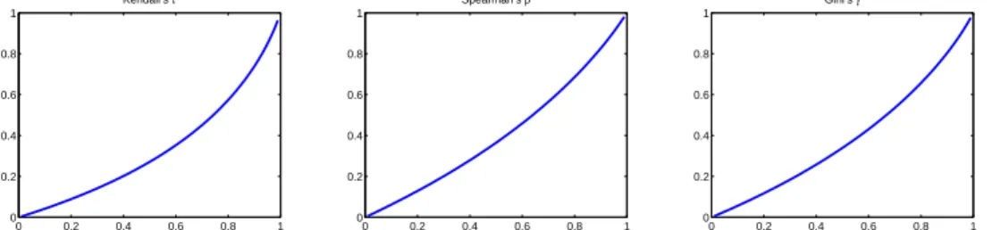
Figure 2, below illustrates the dependence of τ, ρandγ from the parameterα. All curves are strictly monotone increasing and convex. The results from last lemma may be useful to estimate the parameters of the harmonic mean copulas.
0 0.2 0.4 0.6 0.8 1 0 0.2 0.4 0.6 0.8 1 α Kendall’s τ 0 0.2 0.4 0.6 0.8 1 0 0.2 0.4 0.6 0.8 1 α Spearman’s ρ 0 0.2 0.4 0.6 0.8 1 0 0.2 0.4 0.6 0.8 1 α Gini’s γ
Figure 2: Influence ofαon different dependence measures.
5
Derivation of the (upper) tail dependence coefficient
and a generalized TDC estimator
The concept of tail dependence provides, roughly speaking, a measure for extreme co-movements in the lower and upper tail of FX,Y(x, y), respectively and is very useful in financial risk management. Regarding the generalized mean copulas, we focus on the upper tail dependence coefficient (TDC) which is usually defined by
λU ≡ lim u→1−P(Y > F −1 Y (u)|X > FX−1(u)) = limu→1− 1−2u+C(u, u) 1−u ∈[0,1] (5.1)
noting that λU is solely depending on the copula and not on the marginal distributions. Coles et al. (1999) provide an asymptotically equivalent version of (5.1),
λU = 2− lim u→1−
logC(u, u)
log(u) . (5.2)
Fischer & D¨orflinger (2006) showed that CG(u, v) from (3.2) is upper tail dependent with TDC λU =α∈[0,1]. This result also holds for the generalized mean copula, as the next lemma shows.
Lemma 5.1. The (upper) TDC of the generalized mean copula is given by λ=α. Proof: Plugging (3.3) into (5.2) and applying l’Hospital’s rule, we obtain
λU = 2− 1 mulim→1− log¡αum+ (1−α)u2m¢ log(u) = 2− 1 mulim→1− u(mαum−1+ 2m(1−α)u2m−1) αum+ (1−α)u2m = 2−(2−α) =α. ¤
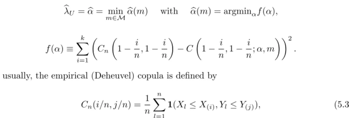
Hence, the upper TDC λU is solely determined by the parameter αand not by m. This allows to construct a generalized TDC-estimator which includes the Dobric-Schmid (2005)
estimator form= 1 and the Fischer-D¨orflinger (2006) estimator for m= 0 as special case. The main idea is simply as follows: At first, approximate the unknown ”data-generating” copula C(u, v) by the generalized mean copula C(u, v;α, m). Secondly, choose α and m such that the squared difference between the empirical copulaCn and the generalized mean copula is minimized. For practical purposes, M is assumed to be a discrete subset of R. Noting thatλU of the latter is given by α, choosebλU as solution of
b λU =αb= min m∈Mαb(m) with αb(m) = argminαf(α), f(α)≡ k X i=1 µ Cn µ 1− i n,1− i n ¶ −C µ 1− i n,1− i n;α, m ¶¶2 .
As usually, the empirical (Deheuvel) copula is defined by Cn(i/n, j/n) = 1 n n X l=1 1(Xl≤X(i), Yl≤Y(j)), (5.3)
where n denotes the number of data pairs (X1, Y1), . . . ,(Xn, Yn) and X(i), Y(i) the corre-sponding order statistics.
Finally, we conducted a small simulation study. In order to compare the quality of the new tail dependence estimators, we simulated from a bivariate Student-t copula with 3 degrees of freedom und ρ = 0.2 (Scenario A). In this case, the theoretical upper tail dependence coefficient is approximately 0.178 (for the exact formula we refer to Dobric & Schmid, 2005). In scenario B, random pairs from a rotated Clayton copula with dependence parameter θ = 0.5 are considered. In this case, the theoretical upper TDC is 2−1/θ = 0.25. In each case, n = 2000 random pairs were repeatedly drawn (with N = 1000 repetitions). The corresponding box plots are subject to figure 3.
1 2 3 4 5 6 7 8 0 0.05 0.1 0.15 0.2 0.25 0.3 0.35 Values Column Number 1 2 3 4 5 6 7 8 0.1 0.2 0.3 0.4 0.5 Values Column Number
Figure 3: Estimation results for the tail dependence estimators (Box plots).
Note that the column numbers 1 to 8 belong to the estimators withm=−5 tom= 2. The drawn through line equals the theoretical (true) TDC. From scenarioAit becomes obvious that all TDC-estimator underestimate the true tail dependence parameter. However, the bias becomes smaller asmdeclines. Regarding scenario B, the smallerm the less the bias of the corresponding TDC-estimator.
References
[1] Borwein, J.M.; Borwein, P.B. Pi and the AGM: A Study in Analytic Number Theory and Computational Complexity. Wiley, New York,1987.
[2] Bouy´e, E.; Durrleman, V.; Nikeghbali, A.; Riboulet, G.; Roncalli, T. Copulas for finance - a reading guide and some applications Authors,Working Paper, Credit Lyonais,2000. [3] Bullen, P.S. Handbook of Means and their Inequalities. Kluwer Academic Publishers,
Dordrecht,2003.
[4] Cherubini, U.; Luciano, E.; Vecchiato, W. Copula methods in finance. John Wiley & Sons, Chichester,2004.
[5] Cuadras, C.M.; Aug´e, J. A continuous general multivariate distribution and its prop-erties.Communications in Statistics (Theory and Methods), 10(4), 339-353,1981. [6] Coles, S.; Heffernan, J.; Tawn, J. Dependence measures for extreme value analyses.
Extremes, 2, 339-365,1999.
[7] Dobric, J.; Schmid, F. Nonparametric Estimation of the Lower Tail Dependence l in Bivariate Copulas.Journal of Applied Statistics, 32(4), 387-407,2005.
[8] Drouet Mari, D.; Kotz, S. I.Correlation and Dependence. World Scientific, Singapore, 2004.
[9] Embrechts, P.; McNeil, A.: Straumann, D.: Correlation: Pitfalls and alternatives A short, non-technical article,RISK Magazine,May, 69-71,1999.
[10] Fischer, M.; D¨orflinger, M. A note on a non-parametric tail dependence estimator.
Discussion Paper no. 76, submitted,2006.
[11] Fr´echet, M. Remarque au sujet de la note pr´ec´edente.R. Acad. Sci. Paris,246, 2719-2720,1958.
[12] Nelsen, R.B.An Introduction to Copulas. Springer, Berlin,2006.
[13] Joe, H. Multivariate Models and Dependence Concepts. Chapman & Hall, London, 1999.
[14] Sklar, A. Fonctions de r´epartitions ´a n dimensions et leurs marges. Publications de l’Institut de Statistique de l’Universit´e de Paris,1959, 8(1), 229-231.