Selection of our books indexed in the Book Citation Index in Web of Science™ Core Collection (BKCI)
Interested in publishing with us?
Contact [email protected]
Numbers displayed above are based on latest data collected. For more information visit www.intechopen.com Open access books available
Countries delivered to Contributors from top 500 universities
International authors and editors
Our authors are among the
most cited scientists
Downloads
We are IntechOpen,
the world’s leading publisher of
Open Access books
Built by scientists, for scientists
12.2%
122,000
135M
TOP 1%
154
Trajectory Control of Robot Manipulators Using a Neural Network
Controller
Zhao-Hui Jiang
x
Trajectory Control of Robot Manipulators
Using a Neural Network Controller
Zhao-Hui Jiang
Hiroshima Institute of Technology
Japan
1. Introduction
Many advanced methods proposed for control of robot manipulators are based on the dynamic models of the robot systems. Model-based control design needs a correct dynamic model and precise parameters of the system. Practically speaking, however, every dynamic model has some degrees of incorrectness and every parameter associates with some degrees of identification error. The incorrectness and errors eventually result positioning or trajectory tracking errors, and even cause the system to be unstable. In the past two decades, intensive research activities have been devoted on the design of robust control systems and adaptive control systems for the robot in order to overcome the control system drawback caused by the model errors and uncertain parameters, and a great number of research results have been reported, for example, (Hsia, 1989), (Kou, and Wang, 1989), (Slotine and Li, 1989), ( Spong, 1992), and (Cheah, Liu and Slotine, 2006). However, almost parts of results associate with complicated control system design approaches and difficulties in the control system implementation for industrial robot manipulators.
Recently, neural network technology attracts many attentions in the design of robot controllers. It has been pointed out that multi-layered neural network can be used for the approximation of any nonlinear function. Other advantages of the neural networks often cited are parallel distributed structure, and learning ability. They make such the artificial intelligent technology attractive not only in the application areas such as pattern recognition, information and graphics processing, but also in intelligent control of nonlinear and complicated systems such as robot manipulators (Sanger, 1994), (Kim and Lewis, 1999), (Kwan and Lewis, 2000), (Jung and Yim, 2001) (Yu and Wang, 2001). A new field in robot control using neural network technology is beginning to emerge to deal with the issues related to the dynamics in the robot control design. A neural network based dynamics compensation method has been proposed for trajectory control of a robot system (Jung and Hsia, 1996). A combined approach of neural network and sliding mode technology for both feedback linearization and control error compensation has been presented (Barambones and Etxebarria, 2002). Sensitivity of a neural network performance to learning rate in robot control has been investigated (Clark and Mills, 2000).
In the following, we present a simple control system consisting of a traditional controller and a neural network controller with parallel structure for trajectory tracking control of
16
industrial robot manipulators. First, a PD controller is designed. Second, a neural network with three layers is designed and added to the control system in the parallel way to the PD controller. Finally, a learning scheme used to train the weights of each layer of the neural network is derived by minimizing a criterion prescribed in a quadratic form of the error between a planed trajectory and response of the robot. Control system implementation issue is discussed. Both the motivation function of the neural network and dynamic model used in the calculation of the learning law are simplified to meet practical needs. An industrial manipulator AdeptOne is adopted as an experimental test bed. Trajectory tracking control simulations and experiments are carried out. The results demonstrate effectiveness and usefulness of the proposed control system.
2. Dynamic models of robot manipulators
2.1 Torque-based dynamic modelA torque-based dynamic model of robot manipulator describes relationship between motion and joint torque of the robot without concerning what generates the torque and how. This class of dynamic formulation is most popular and widely used in the control design and simulation of the robot manipulator. Usually, a torque-based dynamic model can be systematically derived by using the Lagrange method as follows
τ θ g θ θ θ H θ θ M( ) ( , ) ( ) (1) where, θRn and τRn are joint variable and torque, M(θ)Rnn is inertia matrix,
n R θ θ θ
H( , ) contains Coriolis and centrifugal forces, and g(θ)Rn denotes
gravitational force.
Remarks: In motion equation (1), M(θ) is a symmetric matrix, and M(θ)2H(θ,θ) is a skew symmetric matrix. These properties of robot dynamics allow one to design the control system on the basis of dynamic model in an easier way.
2.2 Voltage-based dynamics model
In the almost cases of industrial robot manipulators, the torque-based dynamic model cannot be used directly because most industrial manipulators are not functionally designed on the basis of torque/force control but servo control. In the other words, as actuators almost all robot manipulators are equipped with servo motors that are controlled by input voltage not by current. The former results the so-called velocity servo, and the later meets the needs of the torque-based control that may require the torque-based dynamic model. For, the robot with servo-controlled motors, we need to take the characteristics of the motors and servo-units into consideration in the dynamic modeling, parameter identification and control design. Generally, the dynamic model of the motor with a servo unit can be given as follows. i i i i vi i i i i i τ f θ D(θ ) u a R τ a L (2)
For the n-link robot manipulator, the dyanmic characteristics of the motors and servo units can be rewritten in a compact form as
u θ D θ f τ Rα τ Lα1 1 () v (3)
Though rates of amplifiers of the servo units are included in the parameters in the above equation, in the following, we rather like to use the nominal terms of parameters that are often referred directly to a servo motor. udiag(u1,u2,,un) denotes the input voltage of the servo units; Ldiag(L1,L2,,Ln), R diag(R1,R2,,Rn) are matrices of inductance and resistance; and α diag(1,2,,n)is the matrix with the elements being the back electromotive constant of each servo motor; fv diag(fv1, fv2,, fvn) denotes matrix of viscous friction constants, and D(θ)is a diagonal matrix that diagonal elements indicate the constants of Coulomb frictions and electrical dead zones of the motors. Combining (1) and (3) together, after some simple manipulations we obtain
Lˆ(θ)θRˆ(θ,θ)θHˆ(θ,θ)u (4) where ) ( ) ( ˆ θ La 1M θ L (5)
( ) ( , )
( ) ) ( ˆ θ,θ La 1 M θ H θ θ Ra 1M θ R (6)
( , ) ( )
( , ) ( )
) ( ˆ θ,θ La 1 H θ θθ g θ Ra 1 H θ θ θ g θ H (7)3. Control problem statement
Standing on the theoretical view point, the dynamic model given by (4) can be used in model-based control system design with a kind of computed-torque like control method. Implementation of such a control system, however, is difficult to carry out since either acceleration sensors or numerical derivative approaches are necessary for calculating the control input that contains acceleration feedback. Acceleration sensors are not available in industrial robots, and the numerical derivative approaches would result high frequency noises and phase lag. On the other hand, every dynamic model contains more or less modeling errors and/or parameter uncertainties that cause imprecise trajectory tracking in the control based on the dynamic model.
Although what we are discussing here is about high-performance advanced control methods, the practical world that we have to face is that all commercialized industrial robot manipulators associate with built-in traditional PID controllers. However, a significant drawback of the PID control system is that it cannot guarantee a precise tracking result for given dynamic trajectories since such the control system is essentially driven by trajectory error itself.
From the above discussion, we clarified the problems in dynamic trajectory control of robot manipulators, and found two key points for the problem-solving in the dynamic trajectory tracking control system design: one is how to utilize the built-in PID controller of the robot system; another one is how to take the dynamic characteristics of the robot into
consideration in the trajectory control. The neural network provides us with some new options in the control design in many ways: to approximate dynamics and/or inverse dynamics, to compensate dynamic effects, to be a controller itself, etc. In this chapter, we combine the built-in controller and a neural network together to design a new control system for trajectory control of the robot. We aim at high precision trajectory tracking control of the industrial robot manipulators using simple and applicable control method. We design a control strategy with both technologies of PID control a neural network for taking the advantages of both simplicity on design and implementation of a PID controller, and learning capacity of neural network control. The main idea is to establish a control system with the PID controller and a neural network control scheme which are parallel to each other in structure for achieving precise tracking control of dynamic trajectories. The detail description of the control system design yields to the next section.
4. Structures of the robot control system using neural network
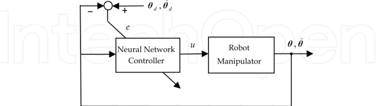
It is usual that the neural network controllers are structurely degined as the feedback controllers in the control system. The neural networks are trained such that the trjactory tracking erorr e converge to zero. Fig.1 and Fig.2 show two kinds of block structures of the
Fig. 1. Structure of a neural network control system with the trajectory error being the input of the neural network.
Fig. 2. Structure of a neural network control system with the state variable being the input of the neural network.
neural network system. In Fig.1, the neural network is driven by the trajectory trcking error, whereas in Fig.2 the neural network is dirven by the states of the robot system.
+ -u Robot Manipulator Neural Network Controller θ θ, d d θ θ , + -u Robot Manipulator Neural Network Controller θ θ, d d θ θ , e e
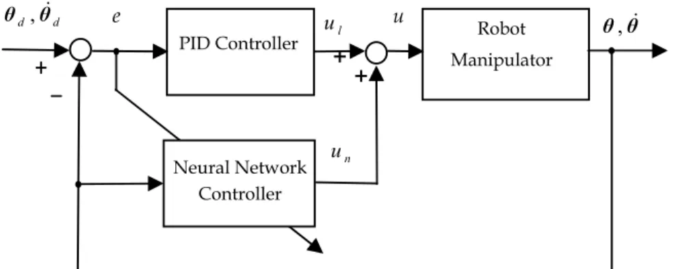
To combine a neural network controller and a built-in PID controller together in parallel, we have two ways according to two structures shown in Fig.1 and Fig.2. In detail, the control system black diagrams are given in Fig. 3 and Fig.4.
Fig. 3. Structure of robot control system with the trajectory error being the input of the neural network.
Fig. 4. Structure of robot control system with the state variable being the input of the neural network.
In control system of Fig.3, what role the neural network controller plays is no more than a controller since the neural network’s input is trajectory error. On the other hand, the neural network controller given in Fig.4 has possibility to work as not only a controller but also a dynamic compensator. The later generates the forces/torques to compensate the gravity and other dynamic forces/torques according to the dynamic trajectories so that the trajectory tracking may be more accurately achieved. In the rest part of this chapter, we will mainly discuss the design of control system that the structure is shown in Fig.4.
5. Control system design
5.1 The control strategyIn the control system shown in Fig.4, the total control scheme is given as follows.
n
l u
u
u (8) l
u is control input of the PID controller, and can be simply described as below.
+ -u + Manipulator Robot PID Controller Neural Network Controller + θ θ, l u n u d d θ θ , e + -u + Manipulator Robot PID Controller Neural Network Controller + θ θ, l u n u d d θ θ , e
consideration in the trajectory control. The neural network provides us with some new options in the control design in many ways: to approximate dynamics and/or inverse dynamics, to compensate dynamic effects, to be a controller itself, etc. In this chapter, we combine the built-in controller and a neural network together to design a new control system for trajectory control of the robot. We aim at high precision trajectory tracking control of the industrial robot manipulators using simple and applicable control method. We design a control strategy with both technologies of PID control a neural network for taking the advantages of both simplicity on design and implementation of a PID controller, and learning capacity of neural network control. The main idea is to establish a control system with the PID controller and a neural network control scheme which are parallel to each other in structure for achieving precise tracking control of dynamic trajectories. The detail description of the control system design yields to the next section.
4. Structures of the robot control system using neural network
It is usual that the neural network controllers are structurely degined as the feedback controllers in the control system. The neural networks are trained such that the trjactory tracking erorr e converge to zero. Fig.1 and Fig.2 show two kinds of block structures of the
Fig. 1. Structure of a neural network control system with the trajectory error being the input of the neural network.
Fig. 2. Structure of a neural network control system with the state variable being the input of the neural network.
neural network system. In Fig.1, the neural network is driven by the trajectory trcking error, whereas in Fig.2 the neural network is dirven by the states of the robot system.
+ -u Robot Manipulator Neural Network Controller θ θ, d d θ θ , + -u Robot Manipulator Neural Network Controller θ θ, d d θ θ , e e
To combine a neural network controller and a built-in PID controller together in parallel, we have two ways according to two structures shown in Fig.1 and Fig.2. In detail, the control system black diagrams are given in Fig. 3 and Fig.4.
Fig. 3. Structure of robot control system with the trajectory error being the input of the neural network.
Fig. 4. Structure of robot control system with the state variable being the input of the neural network.
In control system of Fig.3, what role the neural network controller plays is no more than a controller since the neural network’s input is trajectory error. On the other hand, the neural network controller given in Fig.4 has possibility to work as not only a controller but also a dynamic compensator. The later generates the forces/torques to compensate the gravity and other dynamic forces/torques according to the dynamic trajectories so that the trajectory tracking may be more accurately achieved. In the rest part of this chapter, we will mainly discuss the design of control system that the structure is shown in Fig.4.
5. Control system design
5.1 The control strategyIn the control system shown in Fig.4, the total control scheme is given as follows.
n
l u
u
u (8) l
u is control input of the PID controller, and can be simply described as below.
+ -u + Manipulator Robot PID Controller Neural Network Controller + θ θ, l u n u d d θ θ , e + -u + Manipulator Robot PID Controller Neural Network Controller + θ θ, l u n u d d θ θ , e
dt t d i d p d v l
0 ) ( ) ( ) (θ θ k θ θ k θ θ k u (9)where θd and θdare planned trajectories of joint displacements and velocities, kv, kp, and
i
k are gain matrices. n
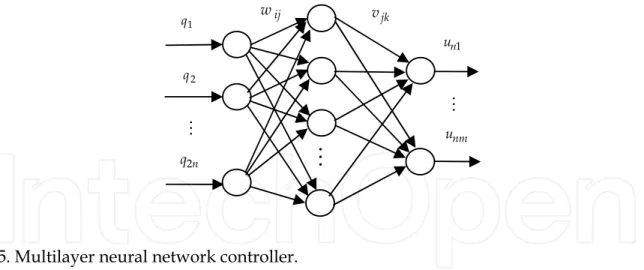
u is the control input of the neural network controller being designed. The structure of neural network controller is shown in Fig. 5. The detail mathematical description of the neural network is given by
f(Wq) V un (10) where T n n n 1 2 R2 2 1, , , , , ] [
q denotes input vector with elements being each joint variable, velocity; m
nm n
n
n [u 1,u 2u ]R
u is output vector, W R2nl and m
l
R
V with their elements being expressed by wij and vjk, are weight matrices from input nodes to the hidden layer and from hidden layer to the output layer; f()Rl is an
activation function vector of the hidden layer with elements being selected as a saturation function, such as a sigmoid function; l is the number of hidden nodes. Though the dimension of robot joint inputs equals joint numbers n, here we denote it as m in order to describe the network controller design clearer.
Fig. 5. Multilayer neural network controller.
2.2 Detail design of the neural network controller
For tracking control of a robot with a designed dynamic trajectory, only the PD controller is not enough to ensure a proper tracking precision. For this reason, we design the neural network controller such that it takes the important part on which the PD controller has shown its limitation and/or powerlessness. In doing so, the neural network controller should be trained in such the way: the trajectory tracking error getting smaller and smaller while training. First, we choose a performance criterion of the whole control system with a quadratic form of the trajectory tracking error and velocity tracking error, as follows.
1 q vjk 1 n u 2 q n q2 nm u ij w
) )( ( 2 1 ) ( ) ( ) ( ) ( q q q q θ θ θ θ θ θ θ θ d d T T 2 1 2 1 E d d d d (11)The weights’ learning algorithm is derived based on the back-propagation approach. The tuning law is to give weights’ increments to be proportional to the negative gradient of the performance criterion with respect to the weights. For updating of the weights between the hidden layer and the output layer, we define an increment as
jk jk jk vE v ( j=1,2,…l; k=1,2,…m ) (12)
where, j and k indicate the one between jth node of the hidden layer and kth node of the output layer , and jk is a constant of proportionality, to be designed as a learning rate. Whereas for the weights between the input layer and hidden layer, we give
ij ij ij wE w ( i=1,2…2n; j=1,2,…l ) (13)
where ij is a learning rate to be designed by the user.
Using the chain rule and noting that the weights are independent withul , the partial
derivative of (12) can be expressed as follows,
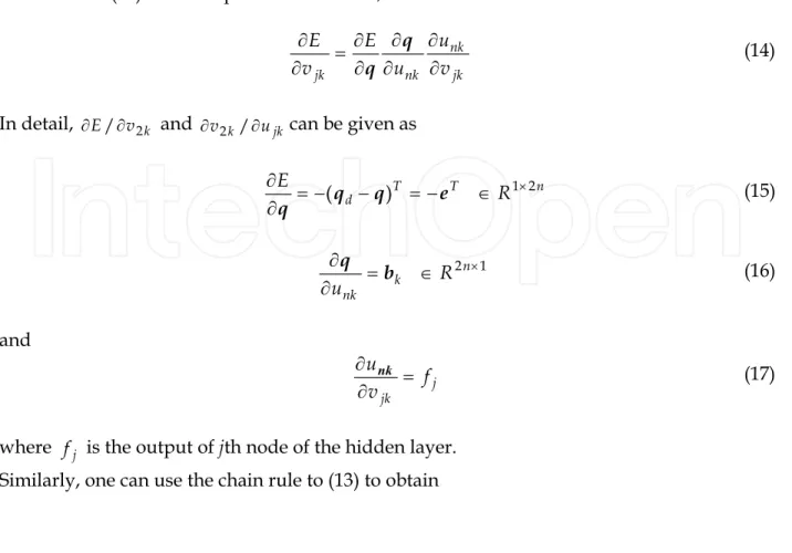
jk nk nk jk v u u E v E q q (14)
In detail, E/v2k and v2k/ujk can be given as
n T T d R E ( ) 12 e q q q (15) 1 2 n k nk R u b q (16) and j jk f v u nk (17)
where fj is the output of jth node of the hidden layer. Similarly, one can use the chain rule to (13) to obtain
dt t d i d p d v l
0 ) ( ) ( ) (θ θ k θ θ k θ θ k u (9)where θd and θdare planned trajectories of joint displacements and velocities, kv, kp, and
i
k are gain matrices. n
u is the control input of the neural network controller being designed. The structure of neural network controller is shown in Fig. 5. The detail mathematical description of the neural network is given by
f(Wq) V un (10) where T n n n 1 2 R2 2 1, , , , , ] [
q denotes input vector with elements being each joint variable, velocity; m
nm n
n
n [u 1,u 2u ]R
u is output vector, W R2nl and m
l
R
V with their elements being expressed by wij and vjk, are weight matrices from input nodes to the hidden layer and from hidden layer to the output layer; f()Rl is an
activation function vector of the hidden layer with elements being selected as a saturation function, such as a sigmoid function; l is the number of hidden nodes. Though the dimension of robot joint inputs equals joint numbers n, here we denote it as m in order to describe the network controller design clearer.
Fig. 5. Multilayer neural network controller.
2.2 Detail design of the neural network controller
For tracking control of a robot with a designed dynamic trajectory, only the PD controller is not enough to ensure a proper tracking precision. For this reason, we design the neural network controller such that it takes the important part on which the PD controller has shown its limitation and/or powerlessness. In doing so, the neural network controller should be trained in such the way: the trajectory tracking error getting smaller and smaller while training. First, we choose a performance criterion of the whole control system with a quadratic form of the trajectory tracking error and velocity tracking error, as follows.
1 q vjk 1 n u 2 q n q2 nm u ij w
) )( ( 2 1 ) ( ) ( ) ( ) ( q q q q θ θ θ θ θ θ θ θ d d T T 2 1 2 1 E d d d d (11)The weights’ learning algorithm is derived based on the back-propagation approach. The tuning law is to give weights’ increments to be proportional to the negative gradient of the performance criterion with respect to the weights. For updating of the weights between the hidden layer and the output layer, we define an increment as
jk jk jk vE v ( j=1,2,…l; k=1,2,…m ) (12)
where, j and k indicate the one between jth node of the hidden layer and kth node of the output layer , and jk is a constant of proportionality, to be designed as a learning rate. Whereas for the weights between the input layer and hidden layer, we give
ij ij ij wE w ( i=1,2…2n; j=1,2,…l ) (13)
where ij is a learning rate to be designed by the user.
Using the chain rule and noting that the weights are independent withul , the partial
derivative of (12) can be expressed as follows,
jk nk nk jk v u u E v E q q (14)
In detail, E/v2k and v2k/ujk can be given as
n T T d R E ( ) 12 e q q q (15) 1 2 n k nk R u b q (16) and j jk f v u nk (17)
where fj is the output of jth node of the hidden layer. Similarly, one can use the chain rule to (13) to obtain
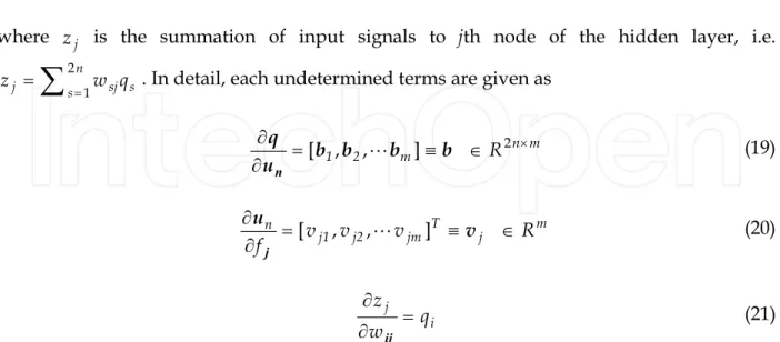
ij j j j j n n T ij w z z f f E w E u u q q (18)
where zj is the summation of input signals to jth node of the hidden layer, i.e.
n
s sj s
j w q
z 2 1 . In detail, each undetermined terms are given as
m n m 2 1 R 2 ] , , [b b b b u q n (19) m j T jm j2 j1 n v v v R f v u [ , , ] j (20) i j q w z ij (21)
In (19), b is a matrix depended on the dynamics of the robot, and will be specified in the next subsection. bk in (16) is the kth column vector of b.
The fourth partial derivative term of right side of (18) can be determined directly using partial derivative fj/zj fj(zj)/zj for a designed activation function fj(zj).
5.3 An implementation issue
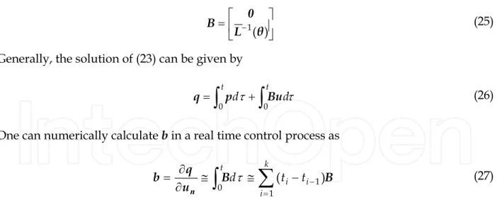
In the design of the neural network controller, since we aimed at trajectory tracking performance of the system, we designed the performance criterion using error’s quadratic form of the inputs of the neural network other than using error’s quadratic form of the outputs of the neural network, though the later is much usual in neural network design. It eventually results the use of dynamics of the system in deriving the learning law with back propagation method since the inputs and outputs of the robot system and neural network controller are contrary to each other. Ignoring the small parameters, usually dynamics (3) can be simplified as u θ θ, h θ θ L( ) ( ) (22) Using q[θT,θT]Tas a state variable vector, above expression can be rewritten as
Bu p q (23) where ) , ( ) ( 1 θ h θ θ L θ p (24) ) ( 1 θ L 0 B (25)
Generally, the solution of (23) can be given by
t d t d 0 0p Bu q (26) One can numerically calculate b in a real time control process asB B u q b
k i i i t t t d 1 1 0 ( ) n (27) where ti indicates the ith sampling time.6. Simulation and experimental studies
6.1 The test bedThe experimental test bed used in this research is an AdeptOne XL robot manipulator shown in Fig.6. It is a SCARA type high performance Direct Drive (DD) industrial robot manipulator possessed with 4 joints. Except the third joint being a prismatic joint, all joints are revolute. Though a closed-loop servo system is built-in by Adept Technology Corporation on the basis of servo units and servo motors, using the Advanced Servo Library the user is allowed to access the D/A converter directly to establish a user-designed close-loop servo system for the development of more advanced control system by V+ language. We developed control software on such the software and hardware environment.
Since the third joint is prismatic and dynamically independent with other joints, control subsystem for the third joint can be designed independently and easily.
Fig. 6. AdeptOne robot manipulator
ij j j j j n n T ij w z z f f E w E u u q q (18)
where zj is the summation of input signals to jth node of the hidden layer, i.e.
n
s sj s
j w q
z 2 1 . In detail, each undetermined terms are given as
m n m 2 1 R 2 ] , , [b b b b u q n (19) m j T jm j2 j1 n v v v R f v u [ , , ] j (20) i j q w z ij (21)
In (19), b is a matrix depended on the dynamics of the robot, and will be specified in the next subsection. bk in (16) is the kth column vector of b.
The fourth partial derivative term of right side of (18) can be determined directly using partial derivative fj/zj fj(zj)/zj for a designed activation function fj(zj).
5.3 An implementation issue
In the design of the neural network controller, since we aimed at trajectory tracking performance of the system, we designed the performance criterion using error’s quadratic form of the inputs of the neural network other than using error’s quadratic form of the outputs of the neural network, though the later is much usual in neural network design. It eventually results the use of dynamics of the system in deriving the learning law with back propagation method since the inputs and outputs of the robot system and neural network controller are contrary to each other. Ignoring the small parameters, usually dynamics (3) can be simplified as u θ θ, h θ θ L( ) ( ) (22) Using q[θT,θT]Tas a state variable vector, above expression can be rewritten as
Bu p q (23) where ) , ( ) ( 1 θ h θ θ L θ p (24) ) ( 1 θ L 0 B (25)
Generally, the solution of (23) can be given by
t d t d 0 0p Bu q (26) One can numerically calculate b in a real time control process asB B u q b
k i i i t t t d 1 1 0 ( ) n (27) where ti indicates the ith sampling time.6. Simulation and experimental studies
6.1 The test bedThe experimental test bed used in this research is an AdeptOne XL robot manipulator shown in Fig.6. It is a SCARA type high performance Direct Drive (DD) industrial robot manipulator possessed with 4 joints. Except the third joint being a prismatic joint, all joints are revolute. Though a closed-loop servo system is built-in by Adept Technology Corporation on the basis of servo units and servo motors, using the Advanced Servo Library the user is allowed to access the D/A converter directly to establish a user-designed close-loop servo system for the development of more advanced control system by V+ language. We developed control software on such the software and hardware environment.
Since the third joint is prismatic and dynamically independent with other joints, control subsystem for the third joint can be designed independently and easily.
Fig. 6. AdeptOne robot manipulator
Focusing on control of the most complex part of the robot, we do not take the third joint into consideration in the control design. The fourth joint is extremely light-weight designed comparing with other joints and its link length is zero. Fourth joint does not cause dynamic coupling to the others. Therefore, we do not take it into consideration as well in control design and experiments.
6.2 Trajectory tracking control simulations
The joint trajectory tracking control simulations were carried out based on a simplified dynamic model of (3). The neural network controller was designed with three layers, four nodes for the input layer and hidden layer respectively, and two nodes for the output layer. The learning scheme was designed using the method given in section IV. The desired joint trajectories are designed using triangle functions with amplitudes to be 45 and 30 degrees for joint1 and joint2. The feedback gain matrices of the PD controller were determined as kp diag(0.6,0.1) , kv diag(0.8,0.3) . Learning rates in (12) and (13) were chosen asj1 0.07 , j2 0.04 (j1,.4) , ij 0.01(i1,,4;j1,.4). Simulations were taken place under Matlab environment.
Fig.7 ~ Fig.10 show an example of the simulations. Fig.7 gives the planned joint trajectories and tracking control results. The broken lines indicate the planned trajectories which are not easy to be seen since they are almost completely covered by the thick lines i.e. the tracking results in fourth time learning. The dotted lines indicate results according PD control only, and the thin lines are first learning results.
Fig.8 gives velocity tracking results with the lines’ types being the same meaning as described for Fig.7. Fig.9 shows control inputs of joint 1, (b) and (c) are control input generated by PD controller and neural network controller, respectively. (a) is the whole control input, i.e. the summation of (b) and (c). Fig.10 shows control inputs of joint 2.
From the simulation results it is seen that using the combined control system with PD controller and neural net work controller high precise joint trajectory tracking performance can be achieved under learning process of the weights of the neural network.
Fig. 7. Simulation results: planned joint trajectories and tracking results.
Fig. 8. Simulation results: planned joint velocity trajectories and tracking results.
Fig. 9. Simulation results: control inputs of joint 1.
6.3 Trajectory tracking control experiments
The joint trajectory tracking control experiments were carried out under almost same conditions of the simulation except the feedback gain matrices were chosen as
) 6 . 0 , 5 . 1 ( diag p
k , kv diag(1.3,0.4), and amplitudes of the trajectories of joint 1 and 2 are planned as 25 and 20 degrees.
Fig.11~Fig.14 show the experimental results. Meaning of each figure stands for the same corresponding to the simulation results shown in the last subsection, as well as the lines in figures.
From the experimental results, it can be seen that though the trajectory tracking accuracy is a little bit lower comparing with the simulation results, the trajectory tracking error becomes less and less when learning time increases. It confirms the effectiveness and usefulness of the proposed control method.
Fig. 11. Experimental results: planned joint trajectories and tracking results.
Fig. 12 Experimental results: planned joint velocity trajectories and tracking results.
Fig. 13. Experimental results: control inputs of joint 1.
Fig. 14. Experimental results: control inputs of joint 2. 6.4 Discussion
PID controller controlled robot system is essentially driven by position error or trajectory tracking error. In dynamic trajectory tracking of a robot under PD control, the PD controller plays two important roles: one is motion regulation for guaranteeing stability of the robot system; another one is to generate force/torque required by the dynamic trajectory to drive the robot such that it would follow the trajectory. The latter needs a big enough tracking error in order to generate actuating force/torque required by the trajectory for the robot. From the simulation results one can see that the tracking error significantly decreases as learning time increases while the control inputs generated by the neural network controller. Comparing Fig.9 (b) with (c) or Fig.10 (b) with (c) it can be interestingly found that learning for four times the neural network controller took PD controller over and played the main role in generating actuation voltages for the robot. On the other hand, in the experimental
results Fig.13 and Fig.14 “the roles changing” seems not as evident as in their simulation counterparts. The reason lies on a fact that we had added the dead-zone compensating inputs into PD control inputs.
Standing on the dynamics point of view, with the same tracking accuracy to a designed dynamic trajectory, the whole control input should be the same judging with the same unit of the input (whatever it counted by torque/force or voltage) regardless what kind of control method is adopted. In robot control with neural network, it is a popular way to use a neural network to approximate dynamics of the robot rather than use it as a controller itself. From the simulation and experimental results, it can be concluded that the neural network controller proposed in this paper not only plays the role as a controller but also play the role to generate force/torque required by dynamic trajectories just as an approximated dynamic model using neural network in computed torque control.
Though the results given here are limited on 4th time learning for the simulation and 6th time learning for the experiment, we carried out much more simulations and experiments, learning for 20 times, for example. The results show that after some specified time the learning effect will remain unchanged.
7. Conclusions
In this article, we presented dynamic trajectory tracking control of industrial robot manipulators using a PD controller and a neural network controller. Some different kinds strucutres of neural network control systems were discuessed. The neural network controller was designed as a three layers feed-forward network. The learning law of weights of the neural network was derived using a simplified dynamic model of the robot and back propagation approach. Dynamic trajectory tracking control simulations and experiments were carried out using an industrial manipulator AdeptOne XL robot. The results showed the effectiveness and usefulness of the proposed control method. From the simulations and experiments, it was seen that according the increase of learning times the neural network controller took over of the PD controller on playing the role in generating actuating force/torque required by the dynamic trajectory. It also was clarified that the learning effect of the neural network has some limitation, i.e. after some specified time of learning, trajectory tracking accuracy remains unchanged.
8. References
Hsia, T. C .S (1989). A new technique for robust control of servo systems,
IEEE Transactions on Industrial Electronics, Vol. 36, No.1, pp.1-7
Kou, C. Y.; Wang, S. P. (1989). Nonlinear robust industrial robot control,
Transactions ASME, Journal of Dynamic Systems, Measurement and Control, Vol.111, No.1, pp 24-30
Slotine, J. J. E.; Li, W. P. (1989). Composite adaptive control of robot manipulators,
Automatica, Vol. 25, No. 4, p 509-519,
Spong, M. W. (1992). On the Robust Control of Robot Manipulators, IEEE Transactions on Automatic Control, Vol. 37, no. 11, pp. 1782-1786
Cheah, C. C.; Liu C. & Slotine, J. J. E. (2006). Adaptive Tracking Control for Robots with Uncertainties in Kinematic, Dynamic and Actuator Models, IEEE Transactions on Automatic Control, Vol.51 No.6, pp.1024-1029
Kwan, C.; Lewis, F. L. (2000). Robust backstepping control of nonlinear systems using neural networks, IEEE Transactions on Systems, Man, and Cybernetics Part A:Systems and Humans., Vol. 30, No. 6, pp.753-766
Sanger, T. D. (1994). Neural network learning control of robot manipulators using gradually increasing task difficulty, IEEE Transactions on Robotics and Automation, Vol. 10, No. pp.323-333
Jung, S.; Yim, S. B. (2001). Experimental Studies of Neural Network Impedance Control for Robot Manipulators, Proceedings of IEEE International Conference on Robotics and Automation, pp.3453-3458
Yu, W. S.; Wang, G. C. (2001). Adaptive Control Design Using Delayed Dynamical Neural Network for a Class of Nonlinear Systems, Proceedings of IEEE International Conference on Robotics and Automation, pp.3447-3452
Kim, Y. H.; Lewis, F. L. (1999). Neural Network Output Feedback Control of Robot Manipulators , IEEE Transactions on Robotics and Automation, Vol.15, No. 2, pp.301-309
Jung, S.; Hsia, T. C. (1996). Neural Network Reference Compensation Technique for Position Control of Robot Manipulator, IEEE Conference on Neural Network, pp 1735-1741, June
Barambones, O.; Etxebarria, V. (2002). Robust Neural Control for Robotic Manipulators,
Automatica, Vol.38, pp.235-242
Clark, C. M.; Mills, J. K. (2000). Robotic System Sensitivity to Neural Network Learning Rate: Theory, Simulation, and Experiments, The International Journal of Robotics Research, Vol.19,No.10, pp.955-968
ISBN 978-953-307-073-5 Hard cover, 666 pages
Publisher InTech
Published online 01, March, 2010
Published in print edition March, 2010
InTech Europe
University Campus STeP Ri Slavka Krautzeka 83/A 51000 Rijeka, Croatia Phone: +385 (51) 770 447 Fax: +385 (51) 686 166 www.intechopen.com
InTech China
Unit 405, Office Block, Hotel Equatorial Shanghai No.65, Yan An Road (West), Shanghai, 200040, China Phone: +86-21-62489820
Fax: +86-21-62489821
This book presents the most recent research advances in robot manipulators. It offers a complete survey to the kinematic and dynamic modelling, simulation, computer vision, software engineering, optimization and design of control algorithms applied for robotic systems. It is devoted for a large scale of applications, such as manufacturing, manipulation, medicine and automation. Several control methods are included such as optimal, adaptive, robust, force, fuzzy and neural network control strategies. The trajectory planning is discussed in details for point-to-point and path motions control. The results in obtained in this book are expected to be of great interest for researchers, engineers, scientists and students, in engineering studies and industrial sectors related to robot modelling, design, control, and application. The book also details theoretical, mathematical and practical requirements for mathematicians and control engineers. It surveys recent techniques in modelling, computer simulation and implementation of advanced and intelligent controllers.
How to reference
In order to correctly reference this scholarly work, feel free to copy and paste the following:
Zhao-Hui Jiang (2010). Trajectory Control of Robot Manipulators Using a Neural Network Controller, Robot Manipulators Trends and Development, Agustin Jimenez and Basil M Al Hadithi (Ed.), ISBN: 978-953-307-073-5, InTech, Available from: