Optimisation of network systems for gas and water allocation and spot price dynamic modelling.

(1)

Optimisation of network systems for gas and

water allocation and spot price dynamic

modelling

A thesis submitted in fulfilment of the requirements for the degree of Doctor of Philosophy

Jonathan Plummer

Bachelor of Applied Science(Hons.)

School of Mathematical and Geospatial Sciences College of Science, Engineering and Health

(2)

Declaration

I certify that except where due acknowledgement has been made, the work is that of the author alone; the work has not been submitted previously, in whole or in part, to qualify for any other academic award; the content of the thesis is the result of work which has been carried out since the official commencement date of the approved research program; any editorial work, paid or unpaid, carried out by a third party is acknowledged; and, ethics procedures and guidelines have been followed.

(3)

List of Figures

1 Thesis in the general context . . . 1

2 The mass flow rate of gas through a transverse reference plane in unit time 11 3 The flow of gas through a stream tube. . . 12

(7)

6 Schematic of compressors in parallel formation . . . 17

7 Compressor operating envelope . . . 21

8 Pressure diagram for a compressor with no clearance . . . 23

9 The gas pressure decreases as it moves along the pipe due the force of friction 26 10 A directed network with four nodes, five pipes, and three loads . . . 36

11 The sum of flows into a node must equal the sum of flows out of the node. 38 12 A network with three loads, five pipes, and no cycles . . . 41

13 Motion of a system through a control volume (a) . . . 47

14 Motion of a system through a control volume (b) . . . 47

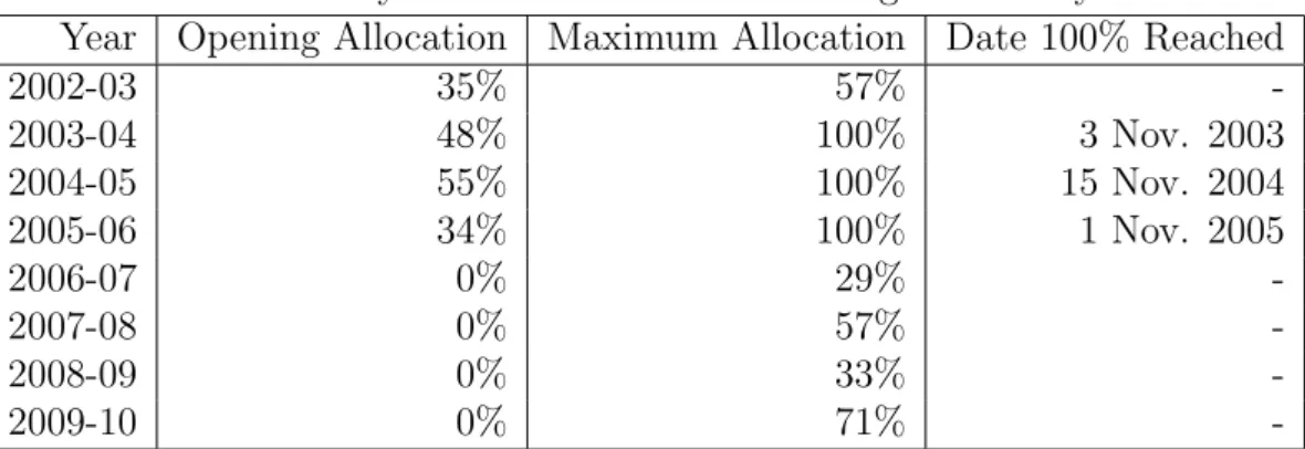
15 The Goulburn-Murray irrigation district. . . 107

16 Water Trading Zones for Victorian Regulated Water Systems. . . 107

17 The Eastern Australian Gas Network. . . 112

18 Water Allocation Trading Price and Volume. . . 141

19 Water Price and Storage Volume. . . 143

20 The Victorian Declared Transmission System. . . 150

21 The weighted average daily price of wholesale gas in the declared wholesale gas market. . . 155

22 A simulation of the weighted average daily price. . . 156

23 Network to be optimised in the minimum shortfall analysis . . . 167

24 Network to be optimised in the minimum cost of supply analysis . . . 179

List of Tables

1 Pipe internal roughness . . . 31

2 Remaining Gas Reserve Estimates (PJ) for Producing Basins . . . 122

3 Typical Composition of Natural Gas . . . 127

4 Summary of seasonal allocations to high reliability shares . . . 139

5 Summary of Water Allocation Prices . . . 140

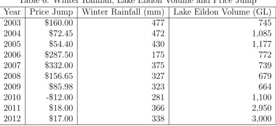
6 Winter Rainfall, Lake Eildon Volume and Price Jump . . . 144

7 Regression Analysis . . . 145

8 Actual Price Jump and Predicted Price Jump . . . 145

9 Paramter estimates and standard errors . . . 156

10 Pipeline daily capacity and tariffs . . . 160

11 Daily capacity at production nodes . . . 162

12 Forecast maximum daily demand (TJ) . . . 163

13 Forecast growth for summer maximum daily demand (TJ) . . . 163

(8)

15 Forecast growth for winter maximum daily demand (TJ) . . . 165

16 Forecast growth for winter maximum daily demand (TJ) . . . 166

17 Projected summer peak day shortfalls (TJ) . . . 170

18 Summer season pipeline utilisation in years 1 to 10 . . . 171

19 Summer season pipeline utilisation in years 11 to 20 . . . 172

20 Projected winter peak day shortfalls (TJ) . . . 174

21 Winter season pipeline utilisation in years 1 to 10 . . . 176

22 Winter season pipeline utilisation in years 11 to 20 . . . 177

23 Amount transported to minimise the cost of supply in the summer season 182 24 Amount produced to minimise the cost of supply in the summer season . 182 25 Affect of rise in production costs at Longford to $4.10/GJ . . . 183

26 Affect of rise in production costs at Longford to $4.40/GJ . . . 184

30 Affect of rise in production costs at Moomba to $4.15/GJ . . . 187

31 Minimising the cost of supply in the winter season . . . 189

32 Minimising the cost of supply in the winter season . . . 190

33 Affect of a rise in production costs at Longford to $4.10/GJ . . . 190

34 Affect of rise in production costs at Longford to $4.75/GJ in the winter season . . . 191

(9)

Summary

Figure 1 shows the contribution to the field provided in this thesis. The study of network allocation systems for gas and water is conducted with the original research (shown in red in Figure 1) placed in context as a logical extension of the existing research.

Figure 1: Thesis in the general context

This thesis studies the network of high pressure gas transmission pipelines in eastern Australia and the network of irrigation channels in the Goulburn-Murray irrigation dis-trict. The objective is to advance the study of network allocation systems. The research questions examined focus on three problems, optimising the delivery of commodities through networks, the optimisation of the cost of supply, and the modelling of prices of commodities that rely on network structures for delivery. A significant part of this research involves the collation of modelling data for the eastern Australian gas network. Three research questions will be addressed.

(10)

The first research problem is to estimate the price of irrigation water at the start of the irrigation season. Water allocated to holders of water entitlements in the Goulburn-Murray irrigation district are traded on a market exchange. This market has matured to the point where new products based on the water allocations can be introduced which is one of the objectives stated in The Intergovernmental Agreement on a National Water Initiative citation. A pricing model for European style option contracts with water allo-cations as the underlying commodity is available in [38], however options could only be considered after the season had commenced since the price of water exhibits large price jumps between seasons. In order to determine appropriate strike prices for the options an initial period of trading would have to take place to allow price discovery. The strike price is a crucial component of the specification of an option as the payoff is determined by the difference of the market price and the strike price. In this thesis the initial price of water allocations at the beginning of the season is estimated using the volume of water stored in Lake Eildon and the winter rainfall at the town of Jamieson upstream of the lake as predictor variables in a regression model. By providing a reliable estimate of the seasons opening water price a series of options on the price of water allocations can be introduced for trading. The benefit of allowing options on water to trade at the beginning of the season is that water uses can lock in a supply of water at an agreed price thus providing some certainty over one of the key inputs into their production.

The second research question addressed is the absence of a model for simulating the spot price of wholesale natural gas sold in the Victorian declared wholesale gas market. In this thesis a model to simulate this price is presented. With this model holders of a portfolio of energy contracts will now have the ability to ascertain the potential losses they may be exposed to in the spot market.

In the third research problem addressed in this thesis, the optimal routing of natural gas to the major demand centres in eastern Australia is addressed. Two formulations are presented with the first focussing on minimising shortfalls on days of simultaneous peak demand across all demand centres. Annual growth factors are applied to current peak day estimates and the model is run for each of the next 20 years and the size of any shortfalls are quantified. The network components that are causing the shortfalls are identified. In the second model the cost of supplying current peak day demand is minimised and the sensitivity of the solution to changes in production costs at supply nodes is discussed. The production costs are the most variable cost in the supply of natural gas. Gas resources

(11)

production costs of different gas basins changes.

The structure of this thesis is arranged as follows. In Section two, the mathematics used in the literature regarding the networks studied is reviewed before the literature itself is discussed in Section three. The networks are discussed in detail in Section four. This section outlines the geographical reach and the physical characteristics of the network, including both the infrastructure that comprises the networks, and the commodities that are transported through them. A particular focus is given to the gas supply chain since gas reservoirs are unique and the gas in one reservoir can be quite different from another. Therefore the process of locating a gas field and processing its raw gas into the natural gas that is traded is worthy of mention as it has a wide variation in costs. In Section five mathematical models are presented and analysed to provide insight into the research problems identified previously, and in Section six the results of the analysis are discussed.

1

An introduction to networks

Networks appear in our lives in both the natural world and the environment we have constructed. A network is quite simply a group of connected points. The points are known as nodes or vertices and the connecting pathways as edges. Networks can be simple, consisting of a few nodes and edges or amazingly complex with millions of nodes and edges. In the following sections some notable types of networks are identified.

Electricity grids are networks consisting of generators, substations and transformers, which are generally represented as nodes, and high voltage transmission wires which form the edges joining the nodes [1]. They have many interesting features to study with one unusual feature being the possibility of cascading failures. One way a cascading failure might occur is if the electricity generated and the load demanded are not in balance causing the mains frequency to speed up or slow down. This instability in the system can cause infrastructure to fail which weakens the system and increases the probability other infrastructure in the system will also fail [42]. However, while network theory can be useful in understanding the structure of the network, it has not been used successfully to explain the complex nature of power grid failures, with most failures usually due to factors such as software bugs or operator error [73].

(12)

Transportation networks include railway lines, airline routes and roads. Commonly the nodes in these networks are geographic locations and the edges are the rail tracks, roads or air routes [73]. This is not always the case however and Sen et al. [95] model the Indian railway network identifying stations with nodes and a train which stops at any two stations as an edge between them, regardless of how many other stations the train may stop at on the way. The logic of this representation is that if a passenger can travel from stationAto stationB then it is a direct link, if the passenger needs to change trains this is not a direct link and their journey would be along two edges of the network.

River networks can be represented using graphs with each waterway being represented by an edge and the junction of two or more as a node. River networks do not have cycles and always form trees. Trees are connected, directed networks without cycles [73]. River networks are also directed networks as the water always flow in one direction. River networks are an important form of two-dimensional branching networks, furthermore they are natural examples of allometry in that the dimensions of different parts of the river network grow with respect with each other [43]. The vascular systems of plants from branching networks with similar scaling features as river systems, with resources necessary for the plant to grow distributed through a hierarchical network structure [116]. The root system of plants follow a similar structure as do many other biological systems such as the cardiovascular and respiratory networks [17].

Delivery and distribution networks include routes used by logistics companies, net-works of sewerage and water pipelines, oil and gas pipeline netnet-works, and netnet-works of irrigation channels that form irrigation districts [73]. The postal service and logistics companies typically have large processing nodes where parcels and mail are sorted and routed to various destinations. The nodes in this type of network may be the local post office or warehouse, and the larger centralised sorting centres, the edges can represent the delivery routes. A vast amount of fresh water is used on irrigated farms and optimising irrigation networks is important as fresh water becomes a scarce commodity. Irrigation networks in there most basic form consist of reservoirs, channels and farms. The channels can be represented as edges of a graph and the reservoirs, farms, gates and other infras-tructure that regulate flow, are represented as nodes. Oil and gas networks consist of drilling rigs, pipelines and refineries. The pipelines may be represented as edges and the drilling rigs and refineries as nodes. Construction costs are high and a typical problem would involve routing oil and gas through existing pipes to the refinery in an optimal

(13)

2

Mathematics and physics of gas networks

The mathematics discussed in this section are used throughout the literature pertaining to gas network optimisation and price modelling. The physical properties of natural gas are discussed and the characteristics of the two main types of compressors used in gas networks presented. Compressors are often analysed in order to minimise the cost of gas transportation. There are many flow equations that have been developed to model gas flow through different types of networks and those featuring most prominently in the literature will be presented. Two types of incidence matrices commonly used to describe network topologies will be stated along with Kirchoff’s laws of flow balance. These topics are necessary for steady state analysis of gas flow networks. Analysing a gas network in its steady state is far more common in the literature than tackling transient analysis, however the basic equations that underpin transient analysis are discussed also.

Topics from stochastic calculus that have been applied to modelling financial assets are mentioned so that a spot price model for natural gas can be developed, in a similar vain the basics of optimisation theory needed for analysis of the gas transmission network are outlined. In this thesis a mathematical model for simulating the spot price of wholesale gas is developed. This model uses results from stochastic calculus which are presented in this chapter. In addition optimisation models are introduced in this thesis to analyse gas flow through the network. The models find the optimal path and optimal quantity of flow for various objective functions. The mathematics underlying these models is stated in this chapter.

2.1

Properties of natural gas

This section briefly outlines some of the fundamental properties of natural gas including temperature, pressure and density. The basic gas laws are then defined followed by the ideal gas law. Viscosity and the Reynolds number of flow are discussed as are the necessary concepts required to define equations for gas flow through pipes. This is followed by a derivation of Bernoulli’s equation and the general flow equation. Friction between the flowing gas and the pipeline is a critical factor in gas network analysis. Therefore a discussion on the friction factor needed for gas flow equations and a way to calculate this

(14)

factor are necessary. The Weymouth equation is one of several equations used to model the gas flow through high transmission gas pipelines. It provides a conservative estimate of the amount of gas able to be transported and is often chosen by researchers for this reason.

2.1.1 Temperature, pressure and density of a gas

The most commonly used parameters to describe the physical conditions under which natural gas is analysed in network analysis are temperature, pressure and density. Col-lectively this is known as the gas state.

The temperature of gas will be represented by T and is measured on the Kelvin (K) temperature scale. In relation to temperature measured in degrees Celsius (C)

T = 273.15 +t◦C (1)

Before providing a definition for pressure we explain the idea of a continuum. A continuum is when the gas molecules are close enough to each other to be considered continuously distributed throughout a region of interest. The mean free path is the average distance a molecule travels before colliding with another molecule, if it is small in comparison to the characteristic dimension of a device, such as a gas pipeline, then the assumption of a continuum is reasonable [83].

Compressive force acting on an area results in pressure. Mathematically, an infinites-imal force ∆F, acting on an infinitesimal area ∆A results in pressure p. Pressure is defined as:

p= lim

∆A→0 dF

dA (2)

Pressure is measured in pascals or kilopascals [kPa]. The pressure of the atmosphere at sea level is 101.3 kPa [83]. Atmospheric pressure is often used as a datum to measure the gauge pressure. Gauge pressure is the pressure measured above the atmospheric pressure

(15)

Mass G is a scalar quantity that measures the amount of matter in a substance. It is measured in kilograms (kg). The mass of a gas is constant and only changes if gas is added or removed, this is known as the principle of conservation of mass. The literature on gas network optimisation frequently refers to the mass flow rate through a pipeline.

Gas volumeV varies with temperature and pressure. As gas is compressible it expands to fill any area available to it. The specific volume of a gas is the volume occupied by its unit mass [96] and is represented mathematically by

v = V

G (3)

The specific volume is measured in [m3_kg−1_].

The density of a gas is the amount that can fit in a given volume. It is the inverse of the specific volume:

ρ= G

V =

1

v (4)

The specific weight γ of a gas is its weight per unit volume:

γ =ρ·g = g

v (5)

whereg is the acceleration due to gravity measured in [ms−2]. Specific weight is measured in [Nm−3_].

2.1.2 Gas laws

An ideal gas is one in which the molecules are considered to be perfectly elastic and in which there is no attraction or repulsion between the gas molecules. An ideal gas obeys Boyle’s law, Charles’ law and the ideal gas equation.

(16)

varies inversely with the absolute pressure: p1 p2 = v2 v1 (6)

Charles’ law states that if the pressure on a gas is held constant, the gas volume is directly proportional to its temperature:

v1 v2

= T1

T2

(7) Also, if the volume is is kept constant, then the gas pressure changes in proportion to its temperature p1 p2 = T1 T2 (8)

By combining Boyle’s law and Charles’ law we have

p1v1 T1 = p2v2 T2 , or pv T = constant (9)

The constant, known as the gas constant, is independent of the state of the gas but does depend on the properties of the gas, thus it is specific for each gas. The gas constant is denoted by R and is measured in units of [Jkg−1K−1]. Rewriting equation 9 as

pv=RT (10)

we have the ideal gas equation which relates the pressure, volume and temperature of a gas. This is the equation of state for an ideal gas. The ideal gas equation approximately represents the behaviour of many gases at conditions close to normal atmospheric tem-peratures and pressures. It is possible to use equation 10 to calculate the following gas processes:

• the constant temperature of isothermal process;

• the constant pressure or isobaric process;

• the constant volume or isometric process;

(17)

The compression or expansion of an ideal gas can be described by the expression:

pvn =C (11)

wheren is called the polytropic exponent and C is a constant. Such a process is called a polytropic process. Equation 11 is sometimes written in logarithmic form as

ln(p) = −n ln(v) +c (12)

A real gas differs more from an ideal gas the more its density increases. The ideal gas equation can be modified in order to match it with the behaviour of gases other than an ideal gas. This is done by defining a factorZ, called the compressibility factor, such that

Z = pv

RT (13)

For an ideal gasZ = 1.0, and the various virial coefficients provide a series of corrections to the ideal-gas behaviour [75].

Boyle’s law and the equation of state are used in [31] to construct an equation to model the volume of gas stored in the pipes of the network during steady state flow. This volume of gas is known as the linepack.

2.1.3 Viscosity

Viscosity, µ, is the resistance to flow of a liquid. The lower the viscosity, the more easily a fluid will flow through a pipe and lower the pressure drop will be. Resistance to flow reveals itself as a shearing stress within a flowing gas and between the flowing gas and the container.

Related to viscosity is the kinematic viscosity. The kinematic viscosity is the absolute viscosity divided by the gas density:

ν= µ

(18)

The dimension of ν is [m2_s−1_{]. The viscosity of a gas depends on its temperature and}

pressure. The viscosity of a gas increases as its temperature increases. Similarly, the viscosity of a gas increases as the pressure increases.

2.1.4 The Reynolds number of flow

The Reynolds number is used to determine the type of flow in a pipe. At low velocities fluid particles move in parallel lines and retain the same relative position at successive cross-sections. This type of flow is known as viscous, streamline or laminar flow. As velocity is increased the particles no longer move in an orderly manner and cease to maintain their relative positions in successive cross-sections, this is known as turbulent flow. When the motion of a fluid particle is disturbed the force of inertia tends to carry it in the new direction while the viscous forces of the surrounding fluid tend to carry the particle in the direction of the stream. In laminar flow the viscous force is sufficient to overcome the force of inertia but in turbulent flow it is not. Therefore the criterion for determining the type of flow is the ratio of the viscous force to the inertial force [44].

Re= Dwρ

µ (15)

where:

D is the inner diameter of the pipe

w is the velocity of the gas

ρ is the density of gas

µis the viscosity.

Laminar flow occurs when the Reynolds number is below 2,000. Laminar flow is typical of low pressure gas distribution systems which are not considered in this thesis. A flow with a Reynolds number in the range 2,000< Re≤4,000 is said to be in the critical region between laminar and turbulent flow. The gas flow in high pressure transmission networks is typically in the fully turbulent region defined as a Reynolds number greater that 4,000. Fully turbulent flow can be further classified as turbulent flow in smooth pipes, turbulent flow in fully rough pipes and transition flow between smooth and fully

(19)

be fully rough in [71]. This is a common assumption when modelling gas transmission networks.

2.1.5 Rate of flow

Figure 2: The mass flow rate of gas through a transverse reference plane in unit time

w

x

AreaA

The mass flow rate is the mass of the gas which passes a transverse reference plane in unit time. The volume per unit time is known as the discharge rate or volume flow rate. Consider a gas flowing with a mean velocity w in a pipe with cross-sectional area A as depicted in Figure 2. In timet a gas particle will travel a distancex, thus:

w= x

t (16)

The volume flow rate Q is given by

Q= Ax

t =Aw [m

3_s−1_] ₍₁₇₎

and the mass flow rate M is given by

M = ρAx

t =ρAw [kgs

(20)

2.1.6 Continuity of flow

Figure 3: The flow of gas through a stream tube.

stream tube section 1 stream tube section 2

w1

AreadA1

flow _w₂

Area dA2

A stream line is a line or curve that is tangential to the velocity of flow at each instant. By definition there is no flow normal to a stream line and so a collection of stream lines are impermeable and form a tube known as a stream tube. If we consider the flow of gas in the stream tube in Figure 3 to be invariant over time, and define the velocity at sections one and two as w1 and w2 and the small cross-sectional areas at sections one

and two asdA1 anddA2 we can derive the continuity equation for steady state flow. The

mass flow rate is given by

M = ρAx

t (19)

and therefore the masses of gas passing through sections one and two in unit time are

dM1 =ρ1w1dA1 and dM2 =ρ2w1dA2 (20)

Furthermore, dM1 = dM2 as there is no gas flow out of the stream tube and the rate of

flow is steady, thus we have that the mass of gas passing through any cross section of the stream tube in unit time is constant. We can sum across all the stream tubes in a pipe

Z dM = Z ρ1w1dA1 = Z ρ2w2dA2 (21)

and assuming average velocities and constant densities across any cross-section we get

M =ρ1w1A1 =ρ2w2A2 (22)

(21)

2.1.7 Bernoulli’s equation

Figure 4: A fluid particle of cross-sectional area A and length dx

dz z reference axis A p p+dp dx a w weight θ dx = particle length a = acceleration p = pressure w = velocity A = area

The total energy of gas flowing through a pipeline consists of various components. Bernoulli’s equation connects the components to form a conservation of energy equation [96]. For an ideal, frictionless, incompressible fluid Bernoulli’s equation can be written as

p ρg +

w2

2g +z = constant (23)

Each component in the Bernoulli equation represents a component of the hydraulic head. The hydraulic head is the energy per unit weight of a fluid. The components are the pressure head, the velocity head and the elevation head. In equation 23 the pressure head is represented by _ρgp, the velocity head by w₂_g2 and the head due to elevation, or potential head, by z.

We can derive Bernoulli’s equation with reference to Figure 4 which shows a fluid particle of cross-sectional area A and length dx. The particle has velocity w and acceleration a, and p denotes pressure. If we assume that the particle is from an ideal frictionless fluid

(22)

then forces acting on the particle are pressure and gravity.

The particle weight is given by

W =Adxρg (24)

and, if we neglect the force of gravity and assume the direction of flow is positive, the pressure on the particle is given by

pA−(p+dp)A=−dpA (25)

The force of gravity in the direction of motion is given by

−Wsinθ =−(ρgAdx)dz

dx (26)

According to Newton’s second law the mass multiplied by the acceleration in the direction of motion is equal to the sum of the forces. Therefore we have

M =ρAdx (27) and a= dw dt = dw dx × dx dt = dw dx ×w (28) Hence −dpA−(ρgAdx)× dz dx =ρAdx×w dw dx (29)

which when divided by

ρgAdx (30) gives − 1 ρg dp dx − dz dx = w g dw dx (31) or − 1 ρg dp dx + w g dw dx + dz dx = 0 (32)

which are sometimes referred to as the Euler equations. Isothermal Euler equations are used the model the gas dynamics within pipes in [63]. For a fluid of constant density equation 32 can be integrated with respect to x to give Bernoulli’s equation [76].

(23)

2.1.8 Steady state flow

Steady state flow is a common assumption in gas network optimisation models. For example it is assumed in [60] when creating a strategic planning model for the construction of gas transmission networks.

As Bernoulli’s equation is a conservation of energy equation, for any two points along a streamline we have p1 ρg + w2 1 2g +z1 = p2 ρg + w2 2 2g +z2 (33)

In reality energy is lost between points one and two due to various factors with friction being predominate in high pressure gas transmission networks. Equation 33 can be rewritten to account for the energy lost by adding an additional term:

p1 ρg + w2 1 2g +z1 = p2 ρg + w2 2 2g +z2+hf (34)

Herehf represents the total pressure lost due to friction between points one and two [76].

In this section the physical properties of natural gas have been outlined and the steady state flow equation stated. An understanding of the flow regime through a pipe is relevant to this work in order to gain an understanding of the common simplifying assumption most researchers employ when studying gas networks.

2.2

Compressors, regulators and valves in gas networks

Compressors, regulators and valves play an important role in gas transmission networks. As gas travels through the pipelines pressure is lost primarily due to friction, compressors restore the pressure difference necessary to keep gas flowing. When gas leaves the high pressure transmission network and enters the lower pressure pipes of the distribution network regulators are needed to reduce the gas pressure. Valves can be open or closed to allow or prevent gas flow through certain pipes in the network, they also provide

(24)

control over the rate of gas flow and to prevent gas from flowing in the wrong direction [76].

In this section the two main types of compressors will be discussed and their basic prop-erties stated. A large part of the research literature focuses on the optimal use and placement of compressors in a gas network. The inclusion of valves and regulators is less common and their function will be covered only briefly. The significance of the compres-sor use is due to the fact that a portion of the gas being transported is consumed by the compressor to drive the compression process.

2.2.1 Compressors

The two types of compressors in high pressure gas transmission networks are centrifugal compressors and positive placement compressors. Centrifugal compressors are less effi-cient than positive displacement compressors but have the advantage of lower capital cost and lower maintenance costs. They are are more commonly used in gas networks due to their operational flexibility. Centrifugal compressors create the pressure necessary for gas transport by using the centrifugal force created by spinning of the compressor wheel which translates the kinetic energy of the gas into pressure energy of the gas. Positive displacement compressors create pressure by allowing gas into a confined space and then reducing the volume of the space thus increasing the gas pressure. The gas is then re-leased at high pressure into the pipeline. They are efficient and able to produce a wide range of pressures [96].

2.2.2 Compressors in series and parallel

Compressor stations generally configure the compressors in series or parallel depending on operation needs. A example of a series configuration is shown in Figure 5. Compressors in series raise the pressure in steps with each compressor compressing the same amount of gas. At the end of each stage of compression the gas temperature rises and it is often

(25)

FlowQ FlowQ

1,080 psi

1,296 psi

Compression ratio = 1.2 Compression ratio = 1.2

Overall compression ratio = 1.44

Figure 5: Schematic of compressors in series formation

Compressors are arranged in parallel to handle large volumes with each compressor han-dling part of the load and producing the same compression ratio [96]. Figure 5 shows an example of compressors operating in parallel. Positive displacement compressors are most often used in parallel as their efficiency falls at lower compression ratios [76].

6,200 psia 30 Mm3_/day 10 Mm3/day 10 Mm3/day 10 Mm3_/day 8,680 psia 30 Mm3/day Compression ratio = 1.4

Figure 6: Schematic of compressors in parallel formation

2.2.3 Centrifugal compressors

Centrifugal compressors compress gas to lower compression ratios than positive displace-ment compressors and this lends them to a series arrangedisplace-ment within the compressor [76].

(26)

The steady flow work done by a centrifugal compressor is given by Lt= Z p2 p1 V dp (35) where:

Lt = overall compressor work (J)

V = volume (M3₎ p = pressure (P a).

In adiabatic compression there is no heat transfer between the gas and the surroundings and the relationship between pressure and volume is given by

pVδ =C (36)

where

δ is the ration of specific heats of gas, Cp

CV

Cp is the specific heats of gas at constant pressure

CV is the specific heats of gas at constant volume

C is a constant. The parameter δ is known as the adiabatic exponent for the gas and ranges in value from 1.2 to 1.4 [96].

From equation 36 we can write

pVδ =p1V1δ (37)

which can be rearranged to give

V =V1 p1 p 1_δ (38) If we substitute equation 38 into equation 35 we have an expression for the total work of an adiabatic compressor: Ladiabatic= Z p2 p1 V dp =V1p 1 δ 1 Z p2 p1 p−1δdp = δ δ−1p1V1 " p2 p1 δ−_δ1 −1 # (39)

(27)

V1 is the initial volume p1 is the suction pressure

p2 is the discharge pressure [76].

In polytropic compression there is no requirement of zero heat transfer between the gas and the surroundings. The relationship between pressure and volume in a polytropic process is given by:

pVn=C (40)

where n is the polytropic exponent and C is a constant [96]. By replacing the adiabatic exponent δ in equation 39 with the polytropic exponent n we have an expression for the work done by a compressor during polytropic compression:

Lpolytropic = n n−1p1V1 " p2 p1 n−_n1 −1 # (41) where

V1 is the initial volume p1 is the suction pressure

p2 is the discharge pressure [76].A value for the polytropic exponent is needed before

equation 41 is of use. The expression for polytropic efficiency, η can be used:

η= n(δ−1)

δ(n−1) (42)

The polytropic efficiency is determined by testing during the manufacturing process [76].

We can calculate the power required by the compressor using

N =M ·∆h (43)

where:

N = power (kW)

M = mass flow (kgs−1₎

(28)

The polytropic efficiency can be written as η= Rp2 p1 vdp ∆h (44) where:

v = specific volume (m3_kg−1_{), thus the expression for the power required during gas}

compression can be written as

N =M

Z p2

p1

vdp· 1

η (45)

Under the assumption that compression is a polytropic process we can calculate the actual power required for gas compression as

N = p1Q1n η(n−1) " p1 p2 n−_n1 −1 # (46) where:

p1, p2 = suction and discharge pressures respectively (P a) Q1 = the inlet flow (m3s−1) [76].

The overall efficiency of the compressor is function of the polytropic efficiency and the mechanical efficiency. If we represent this function as φ we can write equation 46 as:

N = p1Q1n φ(n−1) " p1 p2 n−_n1 −1 # (47)

where the power is measured in watts W [76].

Figure 7 shows the performance curve of a centrifugal compressor that can be driven at different speeds [96]. The flow rate is shown on the horizontal axis and the pressure ratio on the vertical. The dashed curves show the performance at the different operating speeds. The surge line indicated on the left of the operating envelop shows the minimum rate of flow at which the compressor output remains steady for each compression ratio. The limiting curve on the right is sometimes referred to as the stone wall limit. Increasing the flow beyond the stone wall limit does not correspond to an increase in pressure.

(29)

pressure,p2 p1 flow rate, (Qm3_s−1₎ surge line

Allowable operating region

100% speed 90%

80%

70%

Figure 7: Compressor operating envelope

The performance of centrifugal compressors follow the affinity laws which state that the inlet flow and head vary as the as the speed and square of the speed of the compressor. The horsepower needed for compression changes as the cube of the speed [96]. The affinity laws can be summarised by the following equations.

Q2 Q1 = N2 N1 (48) H2 H1 = N2 N1 2 (49) HP2 HP1 = N2 N1 3 (50) where:

Q1 = initial flow rate Q2 = final flow rate

(30)

H1 = initial head H2 = final head

N1 = initial compressor speed N2 = final compressor speed HP1 = initial horsepower HP2 = final horsepower

2.2.4 Positive displacement compressors

Positive displacement compressors increase the gas pressure by reducing the volume in which the gas is confined. They have higher efficiency than centrifugal compressors and can deliver compressed gas at a wide range of pressures [96]. However, positive displacement compressors have lower mechanical efficiencies due to the fact that they have more moving parts [76]. The two main types of positive displacement compressors are rotary screw compressors and reciprocating compressors. Rotary screw compressors use two helical shaped screw that mesh as they rotate, forcing the gas into a smaller volume while reciprocating processors use a piston to reduce the volume and increase the gas pressure. In the remainder of this section I will state the equations governing reciprocating compressor operations.

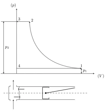
When the piston in a reciprocating compressor moves out (from point 4 to point 1 in Figure 2.2.4) gas is sucked into the cylinder though the suction manifold at constant pressurep1. At point 1 the piston is fully extended the suction valve closes. At this point

the delivery valve opens and the compressed gas is displaced by the piston at constant pressurep2. The change in pressure as the piston moves in and out is shown by the curve

(31)

(p) (V) 1 2 3 4 p2 p1

Figure 8: Pressure diagram for a compressor with no clearance

The actual volume of gas displaced by the piston is given by

Vp =

πD2₁

4 Ln (51)

where:

Vp is the piston displacement (m−3s−1)

D1 is the piston diameter (m) L is the length of stroke (m)

n is the revolutions per second (s−1)

In reality a clearance equal to

c= 0.005L+ 0.5mm (52)

is left so that the piston does not fill the cylinder completely at the bottom of the stroke. The clearance is left to allow for machining tolerances and thermal expansion. The clearance volume, V0, is the total of the space between the closed valves and the

piston and the extra clearance space. The ratio of the clearance volume and the piston displacement volume is

C = V0

Vp

(32)

The actual cylinder capacity, Vs, is the volume of gas actually pumped. The ratio of

the actual cylinder capacity to the piston displacement volume is called the volumetric efficiency and is given by

λV =

Vs

Vp

(54) To calculate the actual volumetric efficiency an allowance must be made for the clearance volume. The actual volumetric efficiency can be calculated using

λV = 1−C " p2 p1 _n1 1 −1 # (55)

where n1 is the polytropic exponent. We can calculate the flow through the compressor

by using equations 54 and 55. The flow equation is

Q1 =λ ( 1−C " p2 p1 _n1 1 −1 #) Vp·s (56)

wheresis the number of cylinders in the compressor. We can also calculate the theoretical power needed for the compression using

N = p1Q1n n−1 " p2 p1 n−_n1 −1 # (57)

The actual power required will be the theoretical power multiplied by a loss factor. The loss factor takes account of the pressure drop due to friction between the moving parts and other mechanical inefficiencies [76].

The procedure to construct the mainline system of a natural gas network is modelled in [91]. This paper concludes that the compression ratio directly affects the investment for compressor stations by determining the number of compressor stations required, the maintenance costs over the life of the network, and the energy consumed in their oper-ation. The required compressor power is also considered a key factor in optimising the number of compressors. The compressor station investment is modelled as a function of the compression ratio and the compressor power. The lifetime cost of fuel consumed by compressor stations is modelled as a function of power and mechanical efficiency in [71]. This paper also notes the large effect the compression ratio has on the economics of the modelled network.

(33)

2.2.5 Valves and regulators

Regulators are used to reduce the pressure of the gas to a specified outlet pressure. They are used at intermediate delivery points on a high-pressure pipeline. Regulators are necessary at the junctions of high pressure transmission pipelines and lower pressure distribution pipelines. Valves in gas networks can be used to redirect flow from one pipeline to another and to shut off parts of a network. This is necessary for maintenance and in emergencies. Valves and regulators are often neglected in gas optimisation models. Two papers include valves and regulators are [54] and [66].

2.3

Steady-state analysis

When the flow of gas through a network does not change over time the network is said to be in steady state. A network in steady state can be described by a set of nonlinear equations

Various formulas have been derived to describe the steady state flow rate of gas in a pipe. These formulas relate the properties of the gas, such as gravity and compressibility factor, with the flow rate, the length and diameter of the pipes, and the distance and the pressure along the pipe [96].

2.3.1 General flow equation

In this section a derivation of the general flow equation

Qn = s π2_R air 64 × Tn pn v u u t h (p2 1−p22)− 2p2 avgSgH ZRairT i D5 f SLT Z (58)

is provided. This derivation references the more detailed derivation found in [76]. The general flow equation is derived from Bernoulli’s equation and makes the following

(34)

as-sumptions.

(1) Steady flow - for a steady flow rate the mass flow rate along the pipe is constant. (2) The cross-sectional area of the pipe is constant.

(3) Isothermal flow - energy is lost due to friction with the pipe wall, this energy is dis-sipated into the surroundings. The gas temperature remains constant.

(4) There is little change in kinetic energy along the pipe. (5) There is constant compressibility of the gas along the pipe.

(6) The Darcy friction equation is valid for the pipe and the friction coefficient along the pipe is constant.

We consider the pipe shown in Figure 9 and note that the gas pressure decreases as it moves along the pipe because of the loss of pressure head needed to overcome the force of friction [76]. The density of the gas also decreases and under the assumptions of steady state flow and constant cross-sectional area we note from equation 22

ρ1w1 =ρ2w2 (59)

that the velocityw must also change along the pipe. Therefore to calculate the frictional resistance we consider a small element of the pipe in Figure 9 and integrate over the entire length to obtain the total head lost. The element we consider is from x to x+dx. We have pressure p at distance x from the start of the pipe and pressure p+dp at distance

x+dx, similarly the velocity is w at distance x and w+dw at distance x+dx.

Figure 9: The gas pressure decreases as it moves along the pipe due the force of friction

L x Q w1 w w+dw w2 Q dx p1 p p+dp p2 g1 g g+dg g2 Datum h=z1−z2

(35)

Bernoulli’s equation across this element as p ρg + w2 2g +z = p+dp ρg + (w+dw)2 2g + (z+dz) +dhf (60)

where hf is the head loss due to friction and z +dz is the change in elevation. The

changes in density and velocity change the kinetic energy by a small amount that can be neglected. We use Darcy’s equation

dhf =

4f D

w2

2gdx (61)

to calculate the head loss due to friction. The pipe diameter is represented by Dand the friction factor by f.

Rearranging equation 60 and including Darcy’s equation gives

−dp= 2f ρw

2

D dx+ρgdz (62)

From equation 22 we see that

w= ρ1

ρ w1 (63)

where ρ=ρ2, and as we are considering isothermal flow we can write p

ρ = p1 ρ1

(64) Therefore the velocity w is given by

w= p1

pw1 (65)

and the density ρ by

ρ= p1

pρ1 (66)

If the expressions for w and ρ are in included in equation 62 and the resulting equation is simplified it can be written as

−p dp= 2f Dρ1p1w 2 1dx+ p2 p1 ρ1g dz (67)

(36)

The state equation 69 was defined earlier as

Z = pv

RT (68)

from which we can see that

p1 = ZRT

v (69)

Substituting this expression for p1 in equation 67 gives

−p dp= 2f Dρ 2 1w 2 1ZRT dx+ p2 ZRTg dz (70)

The pipe in Figure 9 is elevated above the datum line. We can use the average pressure along the pipe, p2

avg., in the term for the potential head due to the distance above the

datum line, _ZRTp2 g dz. We also have from the volume flow rate, equation 17 and the continuity equation, equation 22 that

ρ2₁w2₁ =ρ_n2w_n2 =ρ2_nQ 2 n A2 = ρ2 nQ2n πD2 4 2 (71)

where Ddenotes the pipe diameter and the subscript n denotes the standard conditions for pressure, pn ≈ 0.1M P a and temperature Tn = 288K. Substituting this expression

for ρ2

1w21 into equation 70 gives us

−p dp= 32 π2 f ρ2 nQ2n D5 ZRT dx+ p2 avg ZRTg dz (72)

We can express the density ρn in terms of pn by considering the relationship of the gas

constant for the gas to that of air Rair. At the same temperature and pressure the

compressibility factorZ is unity and the state equations for gas and air can be expressed as

pn =ρnRTn and pn = (ρair)nRairTn (73)

respectively. The specific gravity of a gas S is the ratio of its density to that of air, thus

S = ρn

ρair

= Rair

R (74)

(37)

Then the density of the gas can be written as ρn = pn RTn = SPn RairTn (76) and substituting this equation forρnalong with the equation forR into equation 72 gives

−p dp= 32 π2f Spn RairTn 2 Q2 n D5 ZRair S T dx+ p2_avgS ZRairT g dz (77)

which can be simplified slightly and written as

−p dp= 32 π2 f SZT RairD5 Q2_n pn Tn 2 dx+ p 2 avgS ZRairT gh dz (78)

We then need to integrate along the pipeline fromx= 0 and p=p1 tox=L and p=p2

and solve for the flow rate Qn. The result of the integration is

− p2₂−p2₁ 2 = 32 π2 f SZT RairD5 Q2_n pn Tn 2 L+ p 2 avgS ZRairT gh (79)

and solving for Qn gives the general flow equation

Qn = s π2_R air 64 × Tn pn v u u t h (p2 1−p22)− 2p2 avgSgH ZRairT i D5 f SLT Z (80)

For a horizontal pipeline the general flow equation becomes

Qn=C Tn pn s (p2 1−p22)D5 f SLZT (81) where C = r π2_R air 64 = constant (82)

There are several flow equations used to calculate the pressure lost during gas flow through a pipe, the main difference between them is the expression assumed for f, the friction factor. [76].

(38)

2.3.2 The friction factor

The general flow equation for calculating the pressure drop as gas travels along the pipe requires a numerical value for the friction factor, f [69]. The friction factor is a dimensionless parameter that depends on the Reynolds number and the relative roughness of the pipe wall when the flow through the pipe is fully turbulent. The relative roughness is obtained by dividing the effective roughness of the pipe wall with the diameter of the pipe

relative roughness = e

D (83)

The effective roughness e is also commonly called the absolute roughness or the internal roughness [96]. There are several empirical relationships for calculating the friction fac-tor, in the next section one commonly used equation, the Colebrook-White equation is presented.

2.3.3 The Colebrook-White Equation

The Colebrook-White equation can be used to calculate the friction factor in gas pipelines when the flow is fully turbulent, that is, when the Reynolds number is greater than 4,000.

1 √ f =−2 log10 e 3.7D + 2.51 Re√f (84) where f = friction factor

D = pipe inside diameter

e = absolute pipe roughness

Re = Reynolds number of the flow.

In smooth pipes the value ofe is small and may be neglected, thus the Colebrook-White equation reduces to 1 √ f =−2 log10 2.51 Re√f (85)

(39)

factor can be calculated using 1 √ f =−2 log10 e 3.7D (86) A table of typical friction factors is provided in [96] and reproduced in in Table 1.

Table 1: Pipe internal roughness Pipe material Roughness (mm) Riveted steel 0.9 to 9.0

Welded steel 0.045

Cast iron 0.26

PVC, drawn tubing, glass 0.0015 Concrete 0.3 to 3.0

The Australian Pacific LNG pipeline being constructed as part of an LNG export terminal located at Gladstone consists of welded steel pipe segments. The internal diameter of the pipe is 1,067 mm [107]. An estimate of the friction factor for this pipe would therefore be f = 0.0102.

The friction factor is an integral part of the general gas flow equation however, due to it being defined by a highly nonlinear function it must be solved iteratively or values must be read from a chart. Such charts are known as Moody diagrams. To allow direct calculation of the flow equation approximations to the friction factor are commonly used [69]. The Weymouth equation is one equation used that allow direct calculation of the gas flow through a pipe.

2.3.4 The efficiency factor

The efficiency factor allows for factors other than viscous forces that also reduce the amount of gas flowing through a pipe to be included in calculations. The internal surface of a pipe can have rust scaling or dirt deposits, it may also have welded joins and fittings etc. that increase drag losses as gas flows through the pipe. To account for these factors an effective roughness can be used when calculating the friction factor rather than the

(40)

absolute roughness. Furthermore, the Reynolds number is calculated using assumed values for gas density and viscosity, and the average velocity of gas flow, while the flow equations often use assumed values for specific gravity, compressibility and temperature. All of these variables vary with time and depend on the prevailing conditions during gas flow. Average values of these variables are used in calculations and the resulting errors can be incorporated into the efficiency factor [76].

The efficiency factorE can be included in the expression for the friction factor as follows:

r 1 f =E r 1 ft (87) where f is the actual friction factor and ft is the theoretical friction factor. It may also

be introduced via the general flow equation:

Qn=C Tn pn E s (p2 1−p22)D5 ftSLT Z (88)

Equation 88 can be rearranged to give

p2₁−p2₂ = 1 C pn Tn 2 ftSLT Z D5 1 E2Q 2 n (89) or p2₁−p2₂ =αQ 2 n E2 (90) where α= 1 C pn Tn 2 ftSLT Z D5 (91)

Equation 91 shows that the term p2₁−p2₂ is inversely proportional to the square of the efficiency factor for a given flow equationQn [76].

2.3.5 The Weymouth Equation

The Weymouth equation is used in [92] to model the flow rate through a pipeline. It is appropriate for use in high pressure, large diameter, high flow rate transmission pipelines.

(41)

turbulent flow region [96] Q= 3.7435×10−3E Tb pb p2 1−p22es GTfLeZ 0.5 D2.667 (92) where

Q is the gas flow rate

Tb is the base temperature

pb is the base pressure

Tf is the average gas flow temperature

p1 is the upstream pressure p2 is the downstream pressure

Le is the equivalent length of pipe segment

G is the specific gravity of the gas

Z is the compressibility factor of the gas

e is the internal pipe roughness

D is the diameter of the inside of the pipe

E is the pipeline efficiency factor

2.3.6 The Panhandle A equation

The Panhandle A equation was developed as a refinement of the Weymouth equation and is used in [61] to model gas flow through high pressure pipelines. The equation may be written as: Qn= 7.57×10−4 Tn pn s (p2 1−p22)D5 f SLT Z (93)

The friction factor f is given by

r

1

f = 6.872(Re) 0.073

E (94)

If we assume that the physical parameters of the gas are constant the Reynolds number can be defined using

Re=CQ

(42)

where C is a constant. Using equation 95 the friction factor can also be obtained using r 1 f = 14.94E( SQn D ) 0.073 (96) which is applicable when considering natural gas. Under the further assumption that

Z = 0.95, T = 288K and S = 0.589, equation 93 can be rearranged and written as

p2₁−p2₂ =KQ1_n.854 (97)

where:

K = 18.43 L

E2_D4.854 (98)

The Panhandle A equation is used to model gas flow through pipelines at pressures of over 700 kPa [76].

2.3.7 Pipe equations in general form

Commonly used pipe flow equations can be expressed in a general form as follows. Con-sider any pipe k, the equation of flow from node ito node j can be written as

φ[(Qn)k] =Kk(Qnm1)k =Pi−Pj = ∆Pk (99)

where

φ[(Qn)k] is the flow function for pipe k

Kk is the pipe constant for pipe k

(Qn)k is the flow in pipek

Pi =p2i and Pj =p2j

m1 is the flow exponent. The flow exponent takes on different values depending on the

pressure in the network. For a high pressure network m1 = 1.854 [76].

For the remainder of this paper the terms P and ∆P will be referred to as pressure and pressure-drop respectively, (as opposed to pressure squared and difference squared pressures).

(43)

Equation 99 can be rearranged to give φ0(∆Pk) = (Qn)k= ∆Pk Kk _m1 1 (100) To allow for gas to flow in either direction along the pipe we can make a further modifi-cation and rewrite equation 100 as

(Qn)k=Sij Sij(Pi−Pj) Kk _m1 1 (101) where Sij =    1, if Pi > Pj −1 if Pi < Pj

Equation 101 is the general form of the flow equation for a high pressure gas transmission pipeline [76].

When referring to networks in steady state Q will be used in place of Qn for the sake of

simplicity.

2.4

Network topology

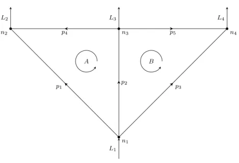
Consider the network shown in Figure 2.4. This network consists of four nodes, {ni :i=

1, . . . ,4}, five pipes {pj : j = 1, . . . ,5} and three loads L1, L2 and L3. Load L1 is the

supply into the network. By convention loads supplied to the network are identified by negative values and load demanded from the network by positive values. For network analysis it is necessary to have at least one reference node at which the pressure is known, typically the pressure is known at a source node and source nodes often serve as reference nodes. In Figure 10 node n1 is the reference node. Reference nodes are

independent, all other nodes and branches are dependent on the reference node. This fact is exploited in the reduced network techniques employed in [88] and [89]. The loads represent demands on the network, they may be positive, negative or zero. Positive loads represent gas supplied to the network, negative loads represent gas supplied from the network to consumers and zero loads represent nodes at which pipes join but gas is neither supplied to or demanded from the network. The total load demanded from

(44)

the network equals the total load supplied to it when the network is operating under steady-state conditions [76]. A B n1 n2 n3 n4 p1 p2 p3 p4 p5 L1 L3 L2 L4

Figure 10: A directed network with four nodes, five pipes, and three loads

Each pipe in the network is assigned a direction arbitrarily, gas flow in that direction is indicated by a positive value for the flow. Gas flow in the opposite direction is indicated by a negative flow value. Finally, connected networks can form closed paths called loops. In Figure 2.4 the pipes p1, p2 and p3 form loop A and pipes p2, p3 and p5 form loop B.

LoopsAand B are independent loops, the third loop consisting of pipesp1,p3,p4 andp5

can be derived from the two independent loops if the common pipe, p2 is discarded [76].

2.4.1 The branch-nodal incidence matrix

The topology of a gas network is easily represented by a matrix. The branch-nodal incidence matrix A = [aij]n×m has one row for each node and one column for each pipe.

(45)

aij = 0 if pipe j is not directly connected to node i. This can be written concisely as aij =         

1, if pipe j enters node i

−1 if pipe j leaves node i

0 otherwise

(102)

2.4.2 The branch-loop incidence matrix

The loops in a gas network can be represented using a branch-loop incidence matrix, B. Each row in the matrix represents an independent loop and each column a pipe. If pipe

j has the same direction as loop i then bij = 1, conversely if pipe j has the opposite

direction as loop i then bij = 1. If pipe j is not part of loop i then bij = 0. This can be

written as: bij =         

1, if pipe j has the same direction as loopi

−1 if pipe j does not have the same direction as loopi

0 otherwise

(103)

The reduced node incidence matrix is defined in the same manner as the branch-nodal incidence matrix but with the rows corresponding to the reference nodes removed. It is written as A1 = [aij]n1×m, where n1 is the number of nodes excluding the reference

node [76].

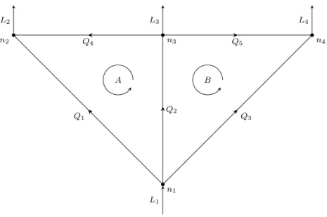
2.4.3 Kirchoff ’s laws

Kirchoff’s first law states the sum of flows into a node must be equal to the sum of flows out of the node [76]. Consider Figure 2.4.3 in which the flows through pipej are denoted byQj.

(46)

A B n1 n2 n3 n4 Q1 Q2 Q3 Q4 Q5 L1 L3 L2 L4

Figure 11: The sum of flows into a node must equal the sum of flows out of the node.

The nodal equations for this network are written as

−Q1 −Q2 −Q3 = −L1

Q1 +Q4 = L2

Q2 −Q4 −Q5 = L3

Q3 +Q5 = L4

(104)

The equations in 104 can be written as

Li = m X j=1 aijQj, i= 1,2, . . . , n (105) or in matrix form as Ln×1 =An×mQm×1 (106) where:

L is the vector of loads at the nodes

Q is the vector of flows in the branches

(47)

In high pressure networks the drop in pressure in the branches can be related to the nodal pressures by the following set of equations

∆P1 = P1 −P2 ∆P2 = P1 −P3 ∆P3 = P1 −P4 ∆P4 = −P2 +P3 ∆P5 = P3 −P4 (107)

which can be written in matrix form as

∆P=−ATP (108)

where

∆Pis the vector of pressure drops

AT _{is the transpose of the branch-nodal matrix}

P is the vector of nodal pressures [76].

If we substitute ∆P into equation 100 we have

Q=φ0(−ATP) (109)

We can then substitute this expression for Q into equation 106 to get

L=A1[φ0(−ATP)] (110)

Equation 110 is the set of nodal equations that describe the gas network. It is solved to obtain values for nodal pressures [76].

Kirchoff’s second law says that there is zero pressure drop around a closed loop. If we denote the change in pressure as ∆p and and adopt the convention that ∆p is positive if the flow direction coincides with the branch direction the loop equations for Figure 2.4.3 are

−∆p1+ ∆p2+ ∆p4 = 0 (111)

for loop A and

(48)

for loop B. The loop equations can be written in general form as m X j=1 bij∆pj, i= 1,2, . . . , k (113) or in matrix form as B∆P=0 (114)

where B is the branch-loop incidence matrix,∆P is the pressure in the branches [76].

2.5

Methods of steady state analysis

Most of the literature analysing gas transmission networks assumes the network is in steady state. For a network to be in steady state the flow of gas through the network must be independent of time. When in steady state the network can be described by a set of nonlinear equations that are also independent of time.

Generally steady state analysis seeks to use known values of the pressure at supply sources and of gas consumption in the nodes to calculate the values of gas flow through pipelines and the pressures at the nodes. The estimates must satisfy the flow rate equation and Kirchoff’s laws [76].

2.5.1 The Newton-nodal method

Equation 110 gives a set of nodal equations that describe a gas network. We can rearrange the equation to get

A1[φ0(−ATP)]−L= 0 (115)

which says mathematically that the sum of flows into and out of the node is equal to zero, this is in accordance with Kirchoff’s first law. The Newton-nodal method starts with an initial estimate of the nodal pressures and seeks to improve it with each iteration. After each iteration the errors in the estimates leave imbalances in the flows through the node.

(49)

has a fixed pressure. The error at each node is denoted by f(P1) where P is the vector

of squared pressures. The set of all nodal errors is represented in a matrix

F(P1) =       f1(P1, P2, . . . , Pn1) f2(P1, P2, . . . , Pn1) .. . fn1(P1, P2, . . . , Pn1)       (116)

where Fdenotes a vector of functions [76].

Equation 115 can be rewritten to include the error functions as

F(P1) =A1[φ0(−ATP)]−L (117)

Equation 117 is solved iteratively and the approximations are improved after each itera-tion using

Pk+1 =Pk₁ + (δP1)k (118)

where k is the number of iterations. We can calculate δP1 using the

Jk(δP1)k =−[F(P1)]k (119) where J =        ∂f1 ∂P1 ∂f1 ∂P2 . . . ∂f1 ∂Pn₁ ∂f2 ∂P1 ∂f2 ∂P2 . . . ∂f2 ∂Pn₁ .. . ... . .. ... ∂fn₁ ∂P1 ∂fn₁ ∂P2 . . . ∂fn₁ ∂Pn₁        (120)

is the Jacobian matrix [76].

The basic approach used in the Newton nodal method can be shown using the simple network shown in Figure 12

(50)

n1 n2 n3 n4 Q1 Q2 Q3 Q4 Q5 L3 L2 L4 Using equation 121 (Qn)k=Sij Sij(Pi−Pj) Kk _m1 1 (121) where Sij =    1, if Pi > Pj −1 if Pi < Pj

as the flow equation, the set of nodal equations can be written as

f2 =S12 S12(P1 −P2) K1 _m1 1 +S32 S32(P3−P2) K4 _m1 1 −L2 f3 =S13 S13(P1 −P3) K2 _m1 1 −S32 S32(P3−P2) K4 _m1 1 −S34 S34(P3−P4) K5 _m1 1 −L3 f4 =S14 S14(P1 −P4) K3 _m1 1 +S34 S34(P3−P4) K5 _m1 1 −L4 (122)

and the Jacobian is

J =        ∂f1 ∂P1 ∂f1 ∂P2 . . . ∂f1 ∂Pn1 ∂f2 ∂P1 ∂f2 ∂P2 . . . ∂f2 ∂Pn1 .. . ... . .. ... ∂fn1 ∂P1 ∂fn1 ∂P2 . . . ∂fn1 ∂Pn1        (123)

(51)

Differentiating equation 122 with respect to P2 gives ∂f2 P2 =− 1 m1 ·S12· S12(P1−P2) K1 1 m₁−1 (P1−P2)−1 − 1 m1 ·S12· S32(P1−P2) K4 1 m₁−1 (P1−P2)−1 (124)

which can be written

∂f2 ∂P2 =− 1 m1 Q1 ∆P2 − 1 m1 Q4 ∆P4 (125) Proceeding in a similar manner gives the remaining values of the Jacobian matrix

J=      Q1 ∆P1 + Q4 ∆P4 − Q4 ∆P4 0 − Q4 ∆P4 Q2 ∆P2 + Q4 ∆P4 + Q5 ∆P5 − Q4 ∆P4 0 − Q4 ∆P4 Q3 ∆P3 + Q5 ∆P5      (126)

which can be written as J = −A1DAT1, where D = diag 1 m1 Qi ∆Pi , for i = 1, . . . , m. Equation 119 is then used to make corrections to the estimates of the nodal pressures [76]. The Newton-nodal method is used in [77] to obtain estimates of the unknown pressure values.

2.5.2 The Hardy-Cross method

Equation 117 can also be solved using the Hardy-Cross method with the main difference being that this method solves for each node separately whereas the Newton method solves the system of equations as a whole. The Hardy-Cross method is used to find the nodal pressures in [29].

The first step is to find initial estimates to the pressures in equation 117. The nodal error for node i is given by

fi(P1) =

m

X

j=1

aij[φ0(−ATP)]−L (127)

The estimates are improved in iterations using

(52)

where:

δP_ik =−(J_iik)−1fi(P1)k (129)

The term Jii is the diagonal term in the Jacobian used in the Newton method

corre-sponding to node i.