Bootstrap multi-step forecasts of non-Gaussian VAR models

This is a postprint version of the following published document:

© Elsevier

This work is licensed under a Creative Commons

Attribution-NonCommercial-NoDerivatives 4.0 International License.

Fresoli, D., Ruiz, E. y Pascual, L. (2015). Bootstrap Multi-step Forecasts of

Non-Gaussian VAR Models. International Journal of Forecasting, v. 31, n. 3, pp. 834-84.

Avalaible in:

http://dx.doi.org/10.1016/j.ijforecast.2014.04.001

Bootstrap multi-step forecasts of non-Gaussian VAR models

Diego Fresoli

a

, Esther Ruiz

a,b,∗

, Lorenzo Pascual

c a_{Dpt. de Estadística, Universidad Carlos III de Madrid, Spain}

b_{Instituto Flores de Lemus, Universidad Carlos III de Madrid, Spain}

c_{EDP-Energías de Portugal, S.A., Unidade de Negócio de Gestão da Energía, Portugal}

a r t i c l e i n f o Keywords: Bias correction DCC model Forecast density Forecast regions High density regions Lag order uncertainty Multivariate forecast Resampling methods

a b s t r a c t

Inthispaper,weestablishtheasymptoticvalidityandanalysethefinitesample perfor-manceofasimplebootstrapprocedureforconstructingmulti-stepmultivariateforecast densitiesinthecontextofnon-GaussianunrestrictedVARmodels.Thisbootstrap proce-dureavoidsthebackwardrepresentation,and,asaconsequence,canbeusedtoobtain multivariateforecastdensitiesin,forexample,VARMAorVAR-GARCHmodels.Inthe con-textofbivariatestationaryVAR(p)models,weshowthatitsfinitesamplepropertiesare comparabletothoseofalternativesbasedonthebackwardrepresentation.Thebootstrap procedureisalsoimplementedinaVAR-DCCmodelwhichlacksabackward represen-tation.Finally,jointforecastdensitiesofUSquarterlyinflation,unemploymentandGDP growthareobtained.

1. Introduction

SinceSims(1980), Vector Autoregressive (VAR) mod-els have been an essential tool for policy making and forecasting in the context of macroeconomic multivari-ate time series; seeStock and Watson(2001) for the ad-vantages and limitations of VAR models. In this paper, we focus on the forecasting ability of VAR models. It is well known that, in practice, VAR forecasts of large macroe-conomic systems may be very imprecise because of the large number of parameters to be estimated relative to the available sample sizes. However, VARs are still very popu-lar when forecasting small or moderate systems in which the parameters can be estimated with an acceptable level of precision. For some selected examples of useful VAR forecasts, seeD’Agostino, Gambetti, and Giannone(2013)

∗_{Correspondence to: Dpt. Statistics, Universidad Carlos III de Madrid,} C/ Madrid 126, 28903 Getafe (Madrid), Spain. Tel.: +34 91 6249851; fax: +34 91 6249849.

E-mail address:[email protected](E. Ruiz).

andMarcellino, Stock, and Watson(2003) for unemploy-ment,Batchelor, Alizadeh, and Visvikis(2007) for interna-tional freight prices,Gupta, Kabundi, and Miller(2011) for US house prices,Baumeister and Kilian(2012) for oil prices,

Polito and Wickens(2012) for fiscal forecasts, andKilian and Vigfusson(2013) for US growth.

Most of the literature dealing with VAR forecasts fo-cuses on marginal point forecasts of each of the variables in the system. However, policy makers and forecasters are increasingly interested in metrics that require joint mul-tivariate forecasts. Komunjer and Owyang(2012) point out the importance of recognizing the multivariate na-ture of most forecasting problems, which has fundamen-tal implications for the prospects of rational expectations in macroeconomic models. Furthermore, joint multivari-ate forecasts are also important when forecasting future values of one variable conditional on particular values of other variables in the system; seeBaumeister and Kilian

(2012),Doan, Litterman, and Sims(1984), andWaggoner and Zha (1999). In order to define spillover measures,

multi-period-ahead forecasts; see alsoKlobner and Wag-ner(2014). On the other hand, the focus of the forecast-ing literature is movforecast-ing from point forecasts to density forecasts that incorporate the uncertainty about the future evolution of the variables of interest; see Bache, Jore, Mitchell, and Vahey (2011), Clark (2011), Diebold, Hanh, and Tay(1999), andJore, Mitchell, and Vahey(2010), among others. Traditionally, a multivariate forecast den-sity for a given horizon can be obtained by assuming Gaussian forecast errors and a known lag order and model parameters. However, it has long been recognized that the parameter uncertainty may be an important issue when dealing with VAR forecasts in practice; seeFair and Shiller

(1990) andLewis and Reinsel(1985) for early references. Furthermore,Kilian(1998a) points out the problems as-sociated with assuming a known lag order when it needs to be estimated. Finally, the empirical evidence suggests that departures from Gaussianity are quite plausible when dealing with economic time series; see for exampleHarvey and Newbold(2003) andKilian(1998b). These departures are a serious concern when forecasting with VAR models, calling into question traditional techniques for construct-ing joint multivariate forecast densities.

Forecast densities that incorporate the parameter and lag order uncertainties without relying on particular as-sumptions on the error distribution can be obtained using bootstrap procedures; seeHolmes, Morris, Tibshirani, and Efron(2003) for an interview with Bradley Efron about the advantages of bootstrap procedures. In the context of fore-casting stationary VAR(p) models, bootstrap methods are introduced byKim(1999), who extends the original pro-cedure proposed byThombs and Schucany(1990) for uni-variate AR(p) processes; seeBerkowitz and Kilian(2000) for a review of bootstrap procedures for time series. Be-cause of the biases associated with the Least Squares (LS) estimator of the VAR parameters,Kim (2001,2004) con-siders bias-corrected forecast regions. The bootstrap pro-cedure proposed byKim(1999) has been implemented for dealing with various different issues in the context of fore-casting using multivariate VAR and periodic state-space models; see, for instance,Grigoletto (2005,2012), Guer-byenne and Hamdi (in press) and Staszewska-Bystrova

(2011). It uses the backward representation (BR) of the VAR model to generate the bootstrap samples used to ob-tain replicates of the estimated parameters. As a conse-quence, its asymptotic validity relies on the assumption of Gaussian errors; seeKim(2001). Given that one of the main attractions of bootstrap procedures is their ability to make predictions in the context of non-Gaussian VAR models, this is an important drawback. Furthermore, boot-strap procedures based on the BR can only be implemented in models with such representations, which excludes, for example, multivariate models with Moving Average (MA)

components or GARCH disturbances; seeAthanasopoulos

and Vahid(2008) andLütkepohl(2006) for forecasting

us-ing VARMA models andKavussanos and Visvikis (2004)

for an empirical example of forecasting with a cointe-grated VAR-GARCH model. Alternatively, Eklund (2007) implements a very simple bootstrap procedure for ob-taining multivariate bootstrap forecasts of several vari-ables of the Icelandic economy that do not require the BR.

However, the bootstrap procedure implemented byEklund

(2007) does not incorporate the parameter uncertainty. Finally, using arguments put forward byPascual, Romo, and Ruiz(2004a) in the context of univariate ARIMA mod-els, one can implement simple bootstrap procedures that incorporate the parameter uncertainty without requiring the BR. For example,Lütkepohl, Staszewska-Bystrova, and Winker(2015), Staszewska-Bystrova and Winker(2013) andWolf and Wunderli(2012) implement the bootstrap procedure originally described byPascual, Ruiz, and Fresoli

(2011)1 for constructing bands for forecast paths. It is important to note that the forward bootstrap procedure implemented in these papers is closely related to the boot-strap procedure proposed byKilian (1998a,b,c)for the con-struction of confidence bands in the context of impulse response functions.

In this paper, we provide a theoretical justification of the forward bootstrap procedure. We establish its asymptotic out-of-sample validity in the context of VAR(p) models, without relying on particular distributions of the forecast errors. Furthermore, Monte Carlo experiments are carried out to analyse its finite sample performance when it is used to construct joint forecast regions. The forward bootstrap regions are compared with traditional and backward bootstrap regions. We show that, regardless of the error distribution, if the VAR(p) model is persistent and the sample size is not very large relative to the number of parameters, the finite sample properties of the bootstrap regions are clearly better than those based on Gaussian densities. Furthermore, we show that, when the VAR(p) model is far from having a unit root and the forecast errors are truly Gaussian, the loss incurred by using bootstrapping is not large, while the improvement in coverage is moderate if the errors are non-Gaussian. In any case, the bootstrap procedures provide similar coverage accuracy levels, regardless of whether they are based on the backward representation or not.

We also illustrate the good performance of the forward bootstrap procedure by constructing forecast densities in the context of a Dynamic Conditional Correlation (DCC) model which does not have a BR. The importance of con-structing forecast regions which take the non-Gaussianity of the variables into account is illustrated by using the forward bootstrap to obtain joint forecast densities of US quarterly inflation, unemployment and growth rates.

The rest of the paper is organized as follows. Section2

focuses the discussion and establishes the notation by describing the traditional and backward bootstrap proce-dures used for constructing forecast densities. Both pro-cedures are illustrated in the context of a non-Gaussian bivariate VAR(2) model. In Section3, the asymptotic va-lidity of the forward bootstrap procedure is established. Section4 reports Monte Carlo results on several bivari-ate VAR models with different parameter configurations, including stationary, persistent and near-cointegrated models. The finite sample performances of the forward bootstrap forecast regions are compared with those of

1_{Pascual et al.(2011) is a previous version of the present paper by the} same authors.

Gaussian and backward bootstrap procedures. Section5

implements the forward bootstrap procedure in data sim-ulated via a VAR-DCC model, while Section6illustrates the results through an empirical application. Finally, Section7

concludes the paper with suggestions for further research.

2. Multi-step forecast densities and regions for VAR models

This section establishes our notation and briefly de-scribes the traditional and backward bootstrap procedures for constructing forecast densities in stationary VAR mod-els.

Consider the following multivariate VAR(p) model of finite lag orderp:

Yt

=

µ

+

Φ1Yt−1

+ · · · +

ΦpYt−p

+

ε

t

,

t

= −

p

+

1

, . . . ,

T

,

(1) whereYt is theN

×

1 vector of observations at time t,

µ

is aN

×

1 vector of constants, andΦi,i

=

1

, . . . ,

p, areN

×

Nparameter matrices that satisfy the stationarity restriction. Finally,

ε

tis a sequence ofN

×

1 independent white noise vectors with distribution functionF_ε, positive definite contemporaneous covariance matrixΣ_ε, and finite fourth order moments.

The point predictor ofYT+hthat minimizes the Mean Squared Forecast Error (MSFE) is its conditional mean, which, in practice, is obtained by substituting the unknown parameters with consistent estimates, as follows:



YT+h|T

=



µ

+



Φ1



YT+h−1|T

+ · · · +



Φp



YT+h−p|T

,

(2) where



YT+j|T

=

YT+j,j

≤

0, and, in this paper,



θ

=

(



µ,



Φ1

, . . . ,



Φp

)

denotes the LS estimator of the param-eters. The MSFE of



YT+h|T

,

denoted byΣ



A



Y

(

h

)

, can be ob-tained using the asymptotic distribution to approximate the parameter uncertainty with all unknown parame-ters substituted by their sample estimates; seeLütkepohl

(1991) for a detailed description. Obviously, the contribu-tion of the parameter uncertainty to the MSFE of



Y_T+h|T de-pends on the dimension of the system,N, the VAR order,

p, and the sample size,T; see for instanceBaillie(1979) andReinsel(1980). As long asNand/orpare big enough relative toT, the effect of the parameter uncertainty can be substantial. However, granted that a consistent estimator is used, the importance of this uncertainty could be small in systems consisting of only a few variables ifT is relatively large; seeRiise and Tjostheim(1984).

If

ε

t is further assumed to be Gaussian for the model in Eq.(1), then theh-step-ahead forecast density can be estimated by

YT+h

∼

N

(



Y_T+h|T

,

Σ



A

Y

(

h

)).

(3)

From Eq.(3), it is possible to obtainh-step-ahead joint ellipsoids for the variables within the system. Constructing

these ellipsoids can be quite demanding when N is

larger than two or three. As a consequence, Lütkepohl

(1991) proposes the construction of forecast regions using Bonferroni cubes based on marginal forecast intervals for each of the variables in the system.

The forecast density in Eq.(3)incorporates the uncer-tainty due to parameter estimation through the asymp-totic distribution, but still relies on Gaussian forecast errors. Therefore, the corresponding intervals and regions could be inadequate when this assumption is not satis-fied. In addition, in this case, the shape of the densities for

h

≥

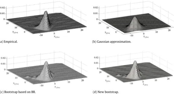
2 is generally unknown. Finally, note that the Gaus-sian forecast densities in Eq.(3)can be misleading in cases where the asymptotic approximation is unreliable; see Du-four and Jouini(2006).

As an illustration, we consider the following non-Gaussian stationary bivariate VAR(2) model previously considered byKim(2001):



y1,t y2,t



=



0

.

9 0

−

0

.

5

−

0

.

7

 

y1,t−1 y2,t−1



+



−

0

.

2 0 0

.

8

−

0

.

1

 

y1,t−2 y2,t−2



+



ε

1,t

ε

2,t



,

(4) where

ε

t

=

(ε

1,t

, ε

2,t

)

′has a

χ

42distribution, standardized

so that

v

ech

(

Σ_ε

)

=

(

1

,

0

.

5

,

1

)

′, with

v

echdenoting the lower-diagonal column stacking operator of a symmetric matrix; seeKilian(1998a) for the adequacy of this distri-bution for representing some macroeconomic time series. The dominant root of the VAR(2) model in Eq.(4)is 0.5, so the model is far from the non-stationary boundary. Panel (a) ofFig. 1displays the true joint one-step-ahead density ofYT+1. After generating a time series of sizeT

=

100,

the VAR(2) parameters are estimated by LS, assuming that the lag order is known. Panel (b) ofFig. 1plots the corre-sponding bivariate density, obtained under the assumption that the forecast errors are jointly Gaussian, as given in Eq.

(3)with



Y_T+1|T

=

(

−

2

.

21

,

−

0

.

27

)

′and

v

ech





ΣA  Y

(

1

)



=

(

1

.

13

,

0

.

59

,

1

.

02

)

′. Comparing panels (a) and (b), it is ob-vious that the Gaussian density fails to capture the asym-metry of the error distribution.

Alternatively, bootstrap procedures can be imple-mented so as to obtain forecast densities that incor-porate the parameter uncertainty without relying on Gaussian forecast errors. In order to take into account the conditionality of VAR forecasts on past observations,Kim

(1999) proposes to obtain bootstrap replicates of the series based on the backward recursion as follows

Y_t∗

=



ω

+

Λ



1Yt∗+1

+ · · · +



ΛpYt∗+p

+



υ

∗ t

,

t

=

T

−

p

, . . . ,

1

,

(5) whereY_t∗

=

Ytfort

=

T

−

p

+

1

, . . . ,

T,

(



ω,



Λ1

, . . . ,



Λp

)

are LS estimates of the backward parameters and

_

υ

∗

t are

random draws with replacement from the empirical dis-tribution function of the backward residuals, re-scaled by the factor [

(

T

−

p

) / (

T

−

(

N

+

1

)

p

−

1

)

]0.5. The bootstrap replicates in Eq.(5)are then used to obtain bootstrap repli-cates of the parameters in Eq.(1), and finally, these are im-plemented to obtain bootstrap replicates ofYT+h

.

Kim(1999) justifies the use of the backward bootstrap procedure in finite samples by suggesting that the asymptotic results ofThombs and Schucany (1990) can be extended to a multivariate framework. When using the backward representation, one can bootstrap from the forward residuals and use the relationship between the

(a) Empirical. (b) Gaussian approximation.

(c) Bootstrap based on BR. (d) New bootstrap.

Fig. 1. Kernel estimates of one-step-ahead forecast densities of a simulated bivariate series withT=100 observations, generated by a stationary VAR(2) model withχ2

4errors.

backward and forward residuals to obtain the bootstrap replicates of the former; see Kim (1997, 1998) for the expression of the backward representation.2In this case, the forward residuals need to be serially independent and identically distributed, but not necessarily Gaussian, for the bootstrap procedure to be asymptotically valid. However, the relationship between forward and backward residuals can be rather complicated in relatively simple VAR models, and many authors resample directly from the backward residuals. The backward errors are only serially independent if the forward errors are Gaussian. Consequently, the asymptotic validity of the bootstrap procedures based on the backward representation relies on the assumption of Gaussian innovations; seeKim(2001).

Another important disadvantage of the backward bootstrap is that it cannot be implemented in models without this representation, which compromises the flexibility and applicability of the procedure.

The backward bootstrap procedure is illustrated by again considering the time series of sizeT

=

100 simulated by the non-Gaussian bivariate VAR(2) model in Eq.(4). Panel (c) of Fig. 1 plots a kernel estimate of the joint backward bootstrap density ofYT+1based onB

=

4999

bootstrap replicates. When comparing this density with its Gaussian counterpart in panel (b), it is clear that the bootstrap can reproduce the asymmetry and is closer to the true density plotted in panel (a) of the same figure.

2 For the simpler expression of the backward representation in which the lag values of the variables in Eq.(1) are substituted by forward values,Chan, Ho, and Tong(2006) andTong and Zhang(2005) show that a necessary condition for the VAR(p) model to have this backward representation is that the covariance matrices Υ(h) =

E

(Yt−E(Yt))(Yt−h−E(Yt))′



are symmetric for allh. This is a very strong restriction which is not likely to be satisfied in real data systems.

3. Forward bootstrap procedure

In this section, we describe the forward bootstrap procedure and establish its asymptotic validity. Its per-formance is illustrated for the non-Gaussian stationary VAR(2) model considered above.

3.1. Description of the algorithm

The forward bootstrap forecast density ofYT+his based on the same assumption that is used to construct fore-cast densities when incorporating the parameter uncer-tainty using the asymptotic distribution, namely, that the sample used to estimate the parameters is independent of the sample used to forecast. In this way, we follow Run-kle(1987) when generating the bootstrap replicates used to estimate the parameters and use the forward instead of the BR. The forward algorithm for obtaining bootstrap replicates ofYT+his a direct generalization of the algorithm proposed byPascual et al.(2004a); seeLütkepohl et al.

(2015),Staszewska-Bystrova and Winker(2013) andWolf and Wunderli(2012) for implementations of the forward bootstrap for obtaining path forecasts in VAR models.

For clarity, we next describe the algorithm.

Step1. After selecting the orderp, obtain LS estimates

of the parameters of model(1) and the corresponding

vector of residuals. Denote by



F

εthe empirical distribution function of the re-scaled residuals.

Step 2. Construct a bootstrap series

{

Y₁∗

, . . . ,

Y_T∗

}

as follows: Y_t∗

=



µ

+



Φ1Y ∗ t−1

+ · · · +



ΦpYt∗−p

+



ε

∗ t

,

t

=

1

, . . . ,

T

,

(6) where

_

ε

∗

t are random draws with replacement from



F εand Y∗ t

=

Yt, for t

= −

p

+

1

, . . . ,

0. Obtain



θ

∗

=

(

_

µ

∗

,



Φ∗ 1

, . . . ,

Φ



∗

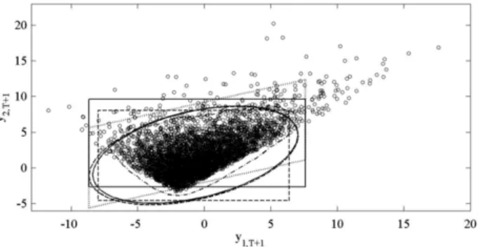
Fig. 2. A realization of sizeR=5000 ofYT+1(◦), generated by a stationary bivariate VAR(2) model withχ42errors, together with 95% one-step-ahead

forecast regions based on a sample sizeT=100: Gaussian ellipsoid and cube (discontinuous lines), bootstrap ellipsoid and cube (continuous line), corrected bootstrap cube (dotted line) and High Density Region (dotted-discontinuous line).

by fitting a VAR(p) model to the bootstrap replicate

{

Y∗ 1

, . . . ,

Y

∗

T

}

.

Step3. Using the model in Eq.(1), with the parameters substituted by their bootstrap estimates, and fixing the last

pobservations of the original series, obtain recursively a bootstrap replicate ofYT+has follows:



Y_T∗_+h|T

=

_

µ

∗

+

Φ



∗ 1



Y_T∗_+h−1|T

+ · · · +

Φ



∗ p



Y ∗ T+h−p|T

+



ε

∗ T+h

,

(7)

with

_

ε

∗_T+hbeing a random draw with replacement from



F ε, and



Y

∗

T+h|T

=

YT+h,h

≤

0.

Step4. Repeat steps 2 and 3Btimes.

It is important to point out that the bootstrap replicates used in step 2 to obtain bootstrap estimates of the parameters are obtained as proposed by Runkle(1987) using the forward expression in Eq. (6) instead of the

backward expression in Eq. (5). However, the last p

observations in the series are still fixed when forecasting the future values in Eq.(7).

To illustrate the implementation of the forward boot-strap procedure and the differences between it and the backward procedure, we again consider the bivariate time series generated by the non-Gaussian stationary VAR(2) model in Eq.(4). Panel (d) ofFig. 1, showing the results for the forward procedure, displays a kernel estimate of the bootstrap joint density ofYT+1, which is very similar to the

density obtained by implementing the backward bootstrap procedure.

Using the algorithm described above, B bootstrap

replicates of YT+h, denoted by

{



Y

∗(1)

T+h|T

, . . . ,



Y

∗(B) T+h|T

}

, are obtained. Their empirical bootstrap distribution can be used to obtain the corresponding bootstrap prediction ellipsoid with probability content

(

1

−

δ)

100% as follows:

ET+h

=



YT+h

|



YT+h

− ¯

Y ∗ T+h|T



S_Yˆ∗

(

h

)

−1

×



YT+h

− ¯

YT∗+h|T



<

Q_K∗



,

(8) where Y

¯

∗

T+h|T is the sample mean of the B bootstrap replicates,S_Yˆ∗

(

h

)

is the corresponding sample covariance,

and Q∗

K is the

(

1

−

δ)

100% percentile of the empirical bootstrap distribution of the quadratic form

[



Y_T∗_+h|T

−

¯

Y_T∗_+h|T

]

S_Yˆ∗

(

h

)

−1

[



Y_T∗_+h|T

− ¯

Y_T∗_+h|T

]

. Furthermore, the Bonfer-roni cube with at least

(

1

−

δ)

100% nominal coverage is given by CT+h

=



YT+h

|

YT+h

∈

N



i=1



q∗_i

(τ) ,

q∗_i

(

1

−

τ)





,

(9) whereq∗

i

(τ)

is the

τ

th quantile of the empirical bootstrap distribution of theith element of



Y_T∗_+h|T. The Bonferroni cubes are defined as in Eq. (9) because they are better suited for dealing with potential asymmetries of the error distribution than the percentile-tintervals; seeHall

(1992). In addition,Kilian(1999) shows that, in the absence of pivotal statistics, as is the case when the VAR process is close to the nonstationary region, bootstrap percentile methods that do not rely on studentized statistics have better coverage accuracies than those based on the percentile-t.

To illustrate the construction of ellipsoids and cubes,

Fig. 2plots the forward bootstrap 95% ellipsoid and the Bonferroni cube in Eqs.(8)and(9)respectively, together with the corresponding regions constructed from the Gaussian density in Eq.(3), both obtained for a particu-lar one-step-ahead realization of the VAR(2) model in Eq.

(4)that is also displayed. We observe that, although the forward bootstrap density is very different from the Gaus-sian density, there are no big differences among the cor-responding ellipsoids, due to the fact that the first two moments involved in their definition do not differ sig-nificantly among the procedures, which estimate simi-lar centers and dispersions of the future values. Note that Y

¯

_T∗_+1|T

=

(

−

2

.

19

,

−

0

.

26

)

′ and

v

ech



S_Yˆ∗

(

1

)



=

(

1

.

11

,

0

.

58

,

1

)

′are very similar to the corresponding quan-tities used to compute the Gaussian ellipsoid. Also, when looking at the bootstrap Bonferroni cube, we can observe that it is located above and to the right of the correspond-ing Gaussian cube, representcorrespond-ing the asymmetries of the joint distribution ofYT+1. Note that, even though the

boot-strap Bonferroni cube is somehow more adequate to repre-sent the asymmetry in the forecast error distribution, it is not satisfactory when constructing forecast regions for sys-tems of correlated non-Gaussian variables, such as those considered in the illustration. Consequently, we explore two further alternatives for the construction of these re-gions. First, we consider the High Density Regions (HDR)

proposed byHyndman(1996) based on kernel estimates of the joint bootstrap density.Fig. 2also plots the 95% HDR computed from the bootstrap replicates,



Y_T∗_+1|T. We can see that the shape of the HDR seems to be a more ad-equate representation of the realization ofYT+1than

ei-ther the ellipsoid or the Bonferroni cube. However, HDR are unfeasible when the dimension of the system is large, as, in this case, there are no satisfactory kernel estima-tors of the bootstrap densities. Consequently, we also ex-plore a simple modification of the Bonferroni cube that takes into account the correlation between the variables in the system. The modified Bonferroni cube is defined by the following four points:



q∗ 1

(τ),

q ∗ 2

(τ)

+

p21,hq∗1

(τ)



,



q∗₁

(

1

−

τ),

q∗₂

(τ)

+

p21,hq∗1

(

1

−

τ)



,

[

q∗₁

(τ),

q∗₂

(

1

−

τ)

+

p21,hq∗1

(τ)

]

, and



q∗₁

(

1

−

τ),

q∗₂

(

1

−

τ)

+

p21,hq∗1

(τ)



, where p21,h

=



σ

∗ 21,T+h

/



σ

2∗ 1,T+h, with



σ

∗ 21,T+h and



σ

2∗ 1,T+h being elements ofS

Y∗

(

h

)

. Note that the proposed trans-formation re-expresses the original cube in a direction defined by the association betweeny1,T+h andy2,T+h, as measured byp21,h. Furthermore, the volume of the mod-ified cube remains unchanged, since the coordinates for the first variable stay the same, while those of the sec-ond variable are transformed by the same amount, ei-therp21,hq∗1

(τ)

orp21,hq∗1

(

1

−

τ)

.Fig. 2plots the modified

Bonferroni cube, which is rotated in the direction of the correlation observed between

_

y∗

1,T+1|T and



y

∗

2,T+1|T, and, as a consequence, gives a more appropriate picture of the values ofy1,T+1andy2,T+1that can be expected one step

ahead.

Before establishing the asymptotic validity of the for-ward bootstrap procedure, we should mention that it can be modified easily by introducing asymptotic stationarity bias corrections of the bootstrap parameters and the en-dogenous lag order bootstrap algorithm, as was proposed byKilian (1998c); seeStaszewska-Bystrova and Winker

(2013) for an implementation of the forward bootstrap al-gorithm using both modifications.

3.2. Asymptotic validity

Consider the stationary VAR(p) model in Eq.(1), where the errors are given by

ε

t

(θ)

=

Yt

−

µ

−

Φ1Yt−1

− · · · −

ΦpYt−p

,

t

=

1

, . . . ,

T

.

(10) In Eq.(10), the errors depend explicitly on the unknown parameters contained in

θ

. If

θ

is estimated by



θ

, the corresponding estimated residuals are given by



ε

t

(



θ)

=

Yt

−



µ

−

Φ



1Yt−1

− · · · −



ΦpYt−p

,

t

=

1

, . . . ,

T

,

(11) which have



F

ε

(



θ)

as the empirical distribution function. The following theorem establishes the asymptotic validity of the empirical bootstrap distribution of



Y_T∗_+h|T, as given in Eq.(7), to approximate the distribution of a future valueYT+h.

Theorem. Let

{

Yt

,

t

=

−

p

+

1

, . . . ,

1

,

2

, . . . ,

T

}

be a realization of a stationary VAR(p) process, defined as in Eq.(1),



θ

be the LS estimator of

θ

, and



Y_T∗_+h|Tbe obtained by following steps1–4in the previous subsection. Then,



Y_T∗_+h|T, conditioned on

{

Yt

,

t

= −

p

+

1

, . . . ,

1

,

2

, . . . ,

T

}

, converges weakly in probability to YT+has T

→ ∞

.

Proof. Following the arguments ofPascual et al.(2004a), consider first the one-step-ahead bootstrap future value given by



Y ∗ T+1|T

=



µ

∗

₊



Φ∗ 1YT

+ · · · +



Φ ∗ pYT−p+1

+



ε

∗ T+1

.

(12) Forh

=

2, we have



Y ∗ T+2|T

=



µ

∗

₊



Φ∗ 1



Y ∗ T+1|T

+ · · · +

Φ



∗ pYT−p+2

+



ε

∗ T+2

.

(13)

Replacing



Y_T∗_+1|Tin Eq.(13)with its expression in Eq.(12), it follows that



Y ∗ T+2|T

=

N0

(



θ

∗

₎

+

N1

(



θ

∗

₎

YT

+ · · · +

Np

(



θ

∗

₎

YT−p+1

+

M1

(



θ

∗

₎



ε

∗ T+1

+



ε

∗ T+2

,

(14)

whereNi

(



θ

∗

)

andM_i

(



θ

∗

)

are appropriately defined contin-uous functions of the estimated parameters.

Proceeding in this way, the following expression is obtained for theh-step-ahead bootstrap forecast:



Y ∗ T+h|T

=

N0

(



θ

∗

₎

₊

N1

(



θ

∗

₎

YT

+ · · · +

Np

(



θ

∗

₎

YT−p+1

+

M1

(



θ

∗

₎



ε

∗ T+1

+

M2

(



θ

∗

₎



ε

∗ T+2

+ · · · +



ε

∗ T+h

,

(15)

where the functionsNi

(



θ

∗

)

andMi

(



θ

∗

)

are different for dif-ferent horizons. Eq.(15)defines the bootstrap future values as a function of the observed realization

{

Y−p+1

, . . . ,

YT

}

, the independent random draws



ε

∗

T+h, and continuous func-tions of the bootstrap parameter estimates



θ

∗.

In order to establish the asymptotic convergence of



Y_T∗_+h|T, we start by considering the terms involvingN_i

(



θ

∗

₎

for which the asymptotic validity of



θ

∗ is needed. The asymptotic validity of the bootstrap LS estimator is estab-lished byBose(1988), who proves the almost sure con-vergence in probability of



θ

∗ to

θ

. Therefore, given that Ni

(



θ

∗

)

are continuous functions of the parameters, it fol-lows thatNi

(



θ

∗

)

p

→

Ni

(θ)

almost surely. Moreover, note thatYT−i+1are fixed values, and consequently, the terms

involvingNi

(



θ

∗

)

YT−i+1

d

→

Ni

(θ)

YT−i+1in probability.

Sec-ond, using the same arguments as before, we can see thatMi

(



θ

∗

)

p

→

Mi

(θ)

almost surely. Finally, consider the terms

_

ε

∗

T+i, which are random draws with replacement from



F

ε

(



θ)

. Using the results ofBickel and Freedman(1981) andFreedman(1984), it is straightforward to prove that

d2

(



F

ε

(



θ),

Fε

(θ))

→

0 in probability asT

→ ∞

, where

d2is a Mallow’s metric. Given that convergence ind2

im-plies weak convergence of the corresponding random vari-ables, it follows that

_

ε

∗

T+i d

→

ε

_T+i in probability. On the other hand,

_

ε

∗

T+iare independent ofMi

(



θ

∗

)

. Consequently, Mi

(



θ

∗

)

_

ε

∗_T+i

d

→

Mi

(θ)ε

T+iby the independence of



ε

∗

T+iand

the bootstrap version of Slutsky’s Theorem. Consequently, all terms in Eq.(15)converge weakly in probability, and, as a result,Y_T∗+h|T

d

Fig. 3. Monte Carlo averages of the empirical coverages of Bonferroni forecast cubes based on the: (i) Gaussian (♦), (ii) Gaussian with asymptotic MSFE (▽), (iii) bootstrap with BR (◦), and (iv) new bootstrap () densities, for a stationary VAR(2) model (first row), a persistent VAR(5) model (second row) and a near-cointegrated VAR(10) model (third row) withT=100 and Gaussian (first column), Student-5 (second column) andχ2

4(third column) errors.

Nominal coverage: 95%.

Before concluding this section, it is important to remark that, even though asymptotic validity is established for centered residuals,Stine(1987) shows that it is still valid if they are also re-scaled. Furthermore, the asymptotic bias correction of the parameters proposed byPope(1990) does not alter the asymptotic validity of our procedure, since the bias and its bootstrap version areOp

(

T−1

)

; seeKilian (1998c) for further details. Finally, Kilian (1998a) also shows that the endogenous lag order bootstrap algorithm is still asymptotically valid for standard lag order selection criteria, such as the AIC considered in this paper.

4. Small sample properties

In this section, we carry out Monte Carlo experiments to analyse the finite sample properties of the forward bootstrap procedure and compare them with those of the alternatives. We consider three different bivariate data generating processes (DGP), with different configurations of parameters and lag orders which reproduce stationary, persistent or near-cointegrated processes. DGP1 is the sta-tionary VAR(2) model defined in Eq.(4). DGP2 and DGP3 are a persistent VAR(5) model and a near-cointegrated VAR(10) model, respectively; seeKilian(1998a) for simi-lar specifications which are described in detail in the Ap-pendix. In each DGP, we consider three distributions of the errors, namely Gaussian, Student-5 and

χ

2

4, which are

ad-equately centered and re-scaled. For each of the resulting nine specifications, we generateM

=

2000 replicates of sizesT

=

100 and 300. The sample sizes have been cho-sen to be in concordance with those usually encountered

in practice when forecasting with real macroeconomic se-ries. For each generated series, the lag order is estimated according to the AIC. The maximum lag orders are equal to 12 and 16 forT

=

100 and 300, respectively. After es-timating the lag order, the VAR parameters are estimated by LS and bias-corrected using the asymptotic correction ofPope(1990), taking into account the stationarity restric-tion proposed byKilian(1998a). Forecast densities for hori-zons ofh

=

1

, . . . ,

8 steps ahead are constructed under the assumption of Gaussian errors without parameter un-certainty, and computing the MSFE as in Eq.(3)using the asymptotic approximation. Forecast densities are also con-structed usingB

=

1999 bootstrap replicates obtained by the backward and forward bootstrap procedures. The boot-strap procedures are implemented using the asymptotic bias and endogenous lag order corrections proposed by Kil-ian (1998a,c). In each case, we construct the corresponding 95% ellipsoids and Bonferroni cubes.

We calculate the empirical coverage of each forecast

region based onR

=

5000 future values of the process

YT+h.Fig. 3 plots the averages through the Monte Carlo replicates of the empirical coverages of the Bonferroni regions constructed for all models considered whenT

=

100.3We can observe that, regardless of the distribution of the error and the procedure used to construct the cubes, the average coverages are rather close to the nominal when

3 Results forT = 300 and the ellipsoids are not reported, to save space. For the same reason, we do not report the results without bias and endogenous lag-order corrections. They are qualitatively similar to those reported in this paper. All of these results are available upon request.

dealing with the VAR(2) models considered in this paper. Note that, in this case, the number of parameters is rather small and the roots of the model are far from the non-stationary region. As a consequence, the uncertainty in the LS estimator is not important when constructing the forecast regions. When the errors are non-Gaussian, we can see that the Gaussian coverages are slightly under the nominal, while the bootstrap cubes maintain their accuracy.

The second and third rows of Fig. 3 plot the

cover-ages corresponding to the persistent VAR(5) and near-cointegrated VAR(10) models, respectively. These models are interesting because the number of parameters is rather large and they are close to the non-stationarity bounds. We can observe that the coverages of the two bootstrap cubes are rather similar, regardless of whether they use the BR or the forward representation. The bootstrap cov-erages are very close to the nominal, although they dete-riorate with the forecast horizon in both models, a feature that is more pronounced in the VAR(10) model. This dete-rioration may be due to the fact that this model is close to the non-stationary bounds, and consequently, it may have more difficulties when forecasting in the long run.Fig. 3

also shows that, in the VAR(10) model, incorporating the parameter uncertainty may be important even when the errors are Gaussian. The coverages of the Gaussian cubes in which the MSFEs do not incorporate the parameter uncer-tainty are smaller than those of cubes constructed by any of the procedures that take into account this uncertainty. Also, when the errors are non-Gaussian, the coverages are under-estimated by both cubes based on Gaussian densi-ties.

To summarize, the simulations carried out in this sec-tion show that the forward bootstrap procedure performs better than traditional methods based on Gaussian densi-ties, and performs no worse than the bootstrap procedure based on the BR. In addition, they suggest that, as the per-sistence of the system increases, it becomes important to take the parameter uncertainty into account in order to ob-tain coverages which are close to the nominal ones.

5. Bootstrap forecasts of returns, volatilities and corre-lations in the DCC model

Multivariate GARCH models (MV-GARCH) are useful for representing the dynamic dependence in the second order moments of multivariate time series. Forecasting correlations is a key issue in financial management, deriva-tive pricing models or hedging strategies; see for exam-pleEngle(2009). The asymptotic validity of the forward bootstrap procedure has been established above for lin-ear VAR models. However, given that the bootstrap pro-cedure considered in this paper does not rely on the BR, it can be extended to deal with conditionally heteroscedas-tic models; seePascual, Romo, and Ruiz(2006) andReeves

(2005) for bootstrap procedures in the context of forecast-ing univariate GARCH models. In this section, we show how to use the forward bootstrap procedure to obtain forecast intervals and regions for returns, volatilities and correla-tions in the context of the Dynamic Conditional Correlation

(DCC) model proposed byEngle(2002). This implemen-tation can also be seen as a multivariate extension of the bootstrap procedure proposed byPascual et al.(2006) for univariate GARCH models. The DCC model is a popular MV-GARCH model that simplifies the estimation of the con-ditional covariance by, first, estimating univariate GARCH models for each variable in the system, and, second, esti-mating the conditional correlation matrix using the result-ing standardized residuals.

In order to simplify the exposition, we will present the results for the following VAR(p)-DCC(1, 1) model:

Yt

=

µ

+

Φ1Yt−1

+ · · · +

ΦpYt−p

+

ε

t

ε

t

=

Ht1/2at

,

(16) whereatis a sequence ofN

×

1 independent white noise vectors with an identity covariance matrix, and Ht is a N

×

Npositive definite conditional covariance matrix given by

Ht

=

DtRtDt

,

(17)

withDtbeing a diagonal matrix containing the univariate GARCH(1, 1) conditional standard deviations of each variable in the system, given by

σ

i,t

=



ω

i

+

α

i

ε

i2,t−1

+

β

i

σ

i2,t−1

,

i

=

1

, . . . ,

N

.

(18)

The matrixRt is the conditional correlation matrix of the standardized errors

ε

s

t

=

D

−1

t

ε

t. In order to ensure the positiveness of the correlation matrix, Rt is defined as follows: Rt

=

QtsQtQts

,

(19) where Qt

=

(

1

−

α

−

β)

Q

+

αε

ts−1

ε

s′ t−1

+

β

Qt−1

,

(20)

withQ being the unconditional correlation matrix. Finally,

Qs

tis a diagonal matrix, with its elements being the inverse square root of the elements in the main diagonal ofQt. All of the parameters are assumed to satisfy the stationarity and positivity conditions.

The evolution of the conditional correlation matrix in Eq.(19)is a nonlinear process where

RT+h|T

=

QTs+h|TQT+h|TQTs+h|T (21) and QT+h|T

=

(

1

−

α

−

β)

Q

+

α

ET

(ε

sT+h−1

ε

s′ T+h−1

)

+

β

QT+h−1|T

,

(22) withET

(ε

sT+h−1

ε

s′ T+h−1

)

=

ET

(

RT+h−1

)

. Consequently, the

h-step-ahead forecast of the correlation matrix cannot be solved forward directly so as to provide a convenient method for forecasting. To overcome this problem,Engle and Sheppard (2001) propose using the approximation

ET

[

Rt+h

] =

ET

[

Qt+h

]

. In this case, RT+h can be forecast directly by RT+h|T

=

(

1

−

α

−

β)

Q h−2



j=0

(α

+

β)

j

+

(α

+

β)

h−1RT+1|T

.

(23)

Note that the one-step-ahead forecast of the correlation matrix,RT+1|T, can be solved backward, which results in

RT+1|T

=

Q

+

α

T−1



j=0

β

j

_(ε

T−jD−T−2j

ε

′ T−j

−

Q

).

(24)

On the other hand, the h-step-ahead forecast of the

volatility of each of the returns is given by

σ

2 i,T+h|T

=

ω

i h−2



j=1

(α

i

+

β

i

)

j

+

(α

i

+

β

i

)

h−1

σ

i2,T+1|T

,

i

=

1

, . . . ,

N

.

(25) An analogous expression is valid for the one-step-ahead forecast of theith variance,

σ

2

i,T+1|T, which is given by

σ

2 i,T+1|T

=

ω

i 1

−

α

_i

−

β

_i

+

α

_i T−1



j=0

β

j i



ε

2 i,T−j

−

ω

i 1

−

α

_i

−

β

_i



,

i

=

1

, . . . ,

N

.

(26) Eqs.(24)and(26)show that, given the model parameters, the one-step-ahead forecasts of the conditional variances and correlations depend only on the observed data

{

Y1

, . . . ,

YT

}

.

Using Eqs. (23) and (25), it is possible to construct

HT+h|T, after which, assuming thatatis Gaussian, one can obtain the forecast density ofYT+h, which is given by YT+h

|

Y1

, . . . ,

YT

∼

N

(

YT+h|T

,

HT+h|T

).

(27)

In practice, the parameters in Eqs. (23)and (25)are unknown and must be estimated. The density in Eq.

(27)does not incorporate the parameter uncertainty, and, as a consequence, will underestimate the uncertainty associated with the forecast ofYT+h. In order to estimate the parameters, in this paper, we first estimate the VAR(p)

parameters using LS, assuming that p is known. Then,

as was proposed by Engle (2002), the parameters of

the DCC model are estimated in two steps using the VAR residuals as follows: (i) the parameters involved in each conditional variance equation are estimated in a univariate fashion using Quasi Maximum Likelihood (QML) by maximizing the Gaussian log-likelihood, and (ii) the parameters governing the correlation dynamics are also estimated by QML using the standardized residuals.4

On the other hand, note that, even if the errors were truly Gaussian, the forecast density in Eq.(27)is valid for

h

=

1 and provides an approximation forh

≥

2.

Fur-thermore, when the errors are non-Gaussian, the future densities of returns predicted using Eq.(27)could be inap-propriate. Finally, even assuming Gaussian errors, it is not straightforward to obtain forecast intervals and regions for future volatilities and correlations. The forward bootstrap

4 The procedure can be modified adequately to deal with the cDCC model ofAielli(2013); seeFresoli and Ruiz(2014) for a detailed analysis of the finite sample properties.

procedure can be implemented to deal with the parameter uncertainty and non-Gaussianity of the errors.

Next, we describe the bootstrap procedure for obtain-ing forecast densities of the returns, volatilities and corre-lations associated withYT+h.

Step 1. Select the orders of the VAR and GARCH

components and estimate the model parameters as described above. Obtain



at, which has an empirical distribution function given by



F

a.

Step 2. Recursively obtain bootstrap replicates of the standardized correlated residuals,

_

ε

s_t∗, and the correlation matrix as follows:



ε

s∗ t

=

R ∗1₂ t



a ∗ t

,

t

=

1

, . . . ,

T

,

(28) where

_

a∗

t are random draws with replacement from



F aand R∗ t

=

Qs ∗ t Q ∗ tQs ∗ t with Q_t∗

=

(

1

−



α

−



β)



Q

+



α



ε

s∗ t−1



ε

s∗′ t−1

+



β

Q_t∗₋₁

,

t

=

2

, . . . ,

T

.

The recursion starts withR∗₁

=

Q₁∗

=



Q, where



Qcontains the sample correlations of

{

Y1

, . . . ,

YT

}

.

Step 3. Obtain bootstrap replicates of

ε

t and their variances as follows:

σ

2∗ i,t

=



ω

i

+



α

i

ε

∗2 i,t−1

+



β

i

σ

i2,t∗−1

,

i

=

1

, . . . ,

N

,

t

=

2

, . . . ,

T

,

(29)



ε

∗ i,t

=



ε

s∗ i,t

σ

∗ i,t

,

i

=

1

, . . . ,

N

,

t

=

1

, . . . ,

T

,

(30) where

σ

_i2_,1∗

=



ω

i

/(

1

−



α

i

−



β

i

)

.

Step4. Construct a bootstrap replicate ofYtas follows: Y_t∗

=



µ

+

Φ



1Yt∗−1

+ · · · +



ΦpYt∗−p

+

ε

∗

t

,

t

=

2

, . . . ,

T

,

where



Y_t∗

=

Yt fort

= −

p

+

1

, . . . ,

0. Obtain bootstrap estimates of the parameters



θ

∗

= [

v

ec

(

µ

_

∗

), v

ec

(



Φ∗₁

), . . . ,

v

ec

(

Φ



_p∗

),

_

α

∗

,



β

∗

, . . . ,

_

ω

∗₁

,

_

α

∗₁

,



β

₁∗

, . . . ,

_

ω

∗_N

,

_

α

_N∗

,



β

_N∗

]

and the sample correlation matrix,



Q∗, by fitting Eq.(20)to the bootstrap replicate

{

Y∗

1

, . . . ,

Y ∗

T

}

. Given the bootstrap esti-mates of the parameters,



θ

∗, and the residuals of the fitted VAR(p) model,

{



ε

1

, . . . ,



ε

T

}

, compute the correlations and variances at the forecast originTas follows:



Q_T∗

=



Q ∗

₊



α

∗ T−1



j=0



β

∗j

₍



ε

T−j−1D ∗−2 T−j−1



ε

′ T−j−1

−



Q ∗

₎



σ

2∗ i,T

=



ω

∗ i 1

−



α

∗ i

−



β

_i∗

+



α

∗ i T−1



j=0

+



β

∗j i

×





ε

2 i,T−j−1

−



ω

∗ i 1

−



α

∗ i

−



β

_i∗



,

i

=

1

, . . . ,

N

.

(31) Obtain also the value of the standardized error atT,

_

ε

s_T∗

=

D∗−_T 1

_

ε

T. Keep the values of



Q_T∗,

_

σ

_i,2_T∗,

_

ε

_Ts∗and

_

ε

T.

Step5. Obtain future values of the correlated standard-ized errors and the correlations through the following re-cursions



ε

s∗ T+h|T

=



R ∗1₂ T+h|T



a ∗ T+h (32)



Q_T∗_+h|T

=

(

1

−



α

∗

₋



β

∗

₎



Q∗

+



α

∗



ε

s∗ T+h−1|T

ε

s∗′ T+h−1|T

+



β

∗



Q_T∗_+h−1|T

,

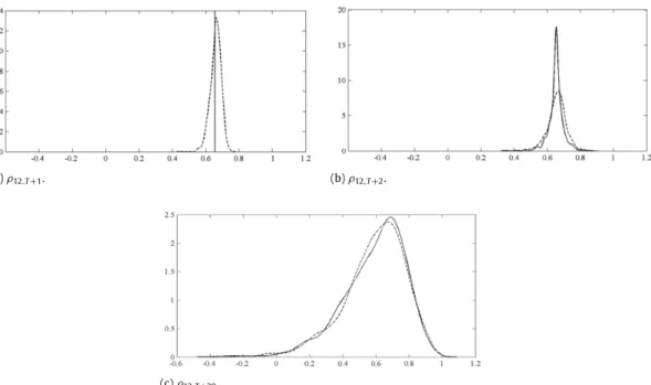
(a)ρ12,T+1. (b)ρ12,T+2.

(c)ρ12,T+20.

Fig. 4. Kernel estimates of the empirical (continuous line) and bootstrap (discontinuous line) densities of (a) one-step-ahead, (b) two-step-ahead and (c) twenty-step-ahead conditional forecasts of the correlations of a bivariate VAR(1)-DCC(1,1) model withT=1000 and Student-7 errors.

where



a

∗

T+hare random draws with replacement from



F a and



R∗_T+h|T

=



Q_Ts∗_+h|T



Q_T∗_+h|T



Q_Ts∗_+h|T with

_

ε

s_T∗_|T

=

_

ε

_Ts∗ and



Q∗

T|T

=



Q_T∗.

Step6. Obtain bootstrap replicates of future errors

ε

T+h and their conditional variances as follows:



σ

2∗ i,T+h|T

=



ω

∗ i

+



α

∗ i



ε

∗2 i,T+h−1|T

+



β

∗ i



σ

2∗ i,T+h−1|T

,

i

=

1

, . . . ,

N

,

t

=

2

, . . . ,

T

,

(33)



ε

∗ i,T+h|T

=



ε

s∗ i,T+h|T

σ

∗ i,T+h|T

,

i

=

1

, . . . ,

N

,

t

=

2

, . . . ,

T

,

(34) where



σ

2∗ i,T|T

=



σ

2∗ i,Tand



ε

∗2 i,T|T

=



ε

∗2 i,T.

Step7. The bootstrap replicate of the future valueYT+h is generated by



Y_T∗_+h|T

=



µ

∗

₊



Φ∗ 1



Y_T∗_+h−1|T

+ · · · +



Φ ∗ p



Y ∗ T+h−p|T

+



ε

∗ T+h|T

,

(35) where



Y_T∗_−j|T

=

Y_T−jforj

>

0. Step8. Repeat steps 2–7Btimes.

It is worth noting that the one-step-ahead bootstrap forecasts,



Q_T∗_+1|Tand

_

σ

_i2_,T∗_+1|T, incorporate only the param-eter uncertainty, since the only components which vary from one bootstrap replicate to another are the bootstrap estimates of the parameters



_

α

∗

,



β

∗



and



_

ω

∗_i

,

_

α

∗_i

,



β

_i∗



, while

{



ε

1

, . . . ,



ε

T

}

is kept fixed among all bootstrap repli-cates. As a consequence, all forecasts of returns, volatilities and correlations are conditional on the observations of the system at timeT.

The bootstrap procedure for the DCC model is il-lustrated for a bivariate VAR(1)-DCC(1, 1) model with Student-7 errors, an intercept

µ

=

(

0

,

0

)

′, and autoregres-sive parameters given by

v

ec

(

Φ1

)

=

(

−

0

.

5

,

0

,

0

.

5

,

0

.

5

)

,

univariate GARCH parameters given by

(ω

1

, α

1

, β

1

)

=

(

0

.

05

,

0

.

05

,

0

.

90

)

and

(ω

2

, α

2

, β

2

)

=

(

0

.

01

,

0

.

10

,

0

.

85

)

,

conditional correlation parameters

(α, β)

=

(

0

.

1

,

0

.

88

)

, and an unconditional correlation matrix

v

ech

(

Q

)

=

(

1

,

0

.

5

,

1

)

. After generating a time series of sizeT

=

1000 via this model, the bootstrap procedure is used to obtain forecast densities of future returns, volatilities and corre-lations. Here, we focus on forecast densities of the cor-relations, because the forecast densities of the levels and their conditional variances have been considered by Pas-cual et al.(2006) in a univariate context already. Fig. 4

plotsh-step-ahead bootstrap densities forh

=

1

,

2 and 20, obtained for the conditional correlation,

ρ

12,t, together with the corresponding empirical densities, where the lat-ter have been obtained by simulating 2000 future values of the process. We can see that the one-step-ahead em-pirical density has all of its mass concentrated at a fixed point. The reason for this is that, in a DCC model,

ρ

12,T+1is

observable with the information available at timeT. How-ever, by incorporating the parameter uncertainty involved in



ρ

12,T+1, one can obtain an estimate of the density of

ρ

12,twhich suggests that the one-step-ahead uncertainty can be rather large. Also note that the observed value of

ρ

12,T+1 is very likely according to this bootstrap density.

Panel (b) ofFig. 4plots the two-step-ahead bootstrap den-sity, together with the empirical density of the realizations of

ρ

12,T+2. We can observe that, as expected, the dispersion

of the bootstrap density is larger than that forT

+

1. How-ever, the empirical density of the two-step-ahead condi-tional correlation is still more concentrated in the center of the distribution than the bootstrap density. Finally, panel (c) ofFig. 4plots the bootstrap and empirical densities for twenty-step-ahead conditional correlations. In this case, we observe that the bootstrap density is a good approxima-tion of the empirical density. It is also important to point out that the uncertainty around

ρ

12,T+20 is so large that

Table 1

Descriptive statistics of quarterly US inflation (π), unemployment (u) and GDP growth (g), observed from 1948Q1 to 2009Q3, withp-values in parentheses.

Series Mean Sd Skewness Kurtosis KD ADFa _{Q(8) Q}

2(8) π 0.91 0.83 0.79 5.43 1478.7 (0.00) −(0.00)3.66 130(0.00).09 129(0.00).45 u 0.56 0.15 0.15 3.45 33.26 (0.08) −(0.07)2.68 890(0.00).00 839(0.00).74 g 0.80 1.02 −0.10 4.20 19.85 (0.00) −(0.00)7.25 55(0.00).49 29(0.00).29 (π,u,g) 1.46 21.19 1669.4 (0.00) a_{MacKinnon’sp-value approximation.}

the correlation could be zero or even negative. Note that the quality of the approximation of the bootstrap density to the empirical density improves as the forecast horizon increases. This is due to the fact that, as we forecast further into the future, the role played by the error uncertainty be-comes more important, to the detriment of the parameter uncertainty. After all, this simulated example underscores the flexibility of the forward bootstrap procedure for deal-ing with more complicated models.

6. Empirical application

In this section, we use the forward bootstrap proce-dure to construct forecast densities of quarterly US infla-tion (

π

t), the unemployment rate (ut) and GDP growth (gt), observed from 1948Q1 to 2011Q3.5Inflation rates are com-puted as usual by

π

t

=

log

(

IPIt

/

IPIt−1

)

×

100, whereIPIis

the Implicit Price Deflator. Unemployment is measured by the civilian unemployment rate. Finally, the GDP growth is given bygt

=

log

(

GDPt

/

GDPt−1

)

×

100, where GDP is

the Real Gross Domestic Product. Where relevant, monthly data have been transformed into quarterly data by tak-ing the observations of the last month of the quarter. The whole sample period has been split into an estimation

pe-riod from 1948Q1 to 2009Q3 (T

=

247) and an

out-of-sample period from 2009Q4 to 2011Q3.Table 1reports the sample mean, standard deviation (sd), skewness and kur-tosis of each of the series during the estimation period, to-gether with the joint measures of skewness and kurtosis proposed byMardia(1970).Table 1also displays the nor-mality test statistics and correspondingp-values based on the bootstrap procedure proposed byKilian and Demiroglu

(2000) and denoted by KD. The normality is always re-jected either individually or jointly at the 10% level.Table 1

also displays the Augmented Dickey-Fuller (ADF) statistics, which reject the non-stationarity hypothesis for all series. Finally, the Box-Ljung statistics of order 8 for the original series and their squares, denoted byQ

(

8

)

andQ2

(

8

)

re-spectively, are displayed in the last two columns ofTable 1. We can observe that there is a dynamic dependence in the conditional mean. However, the Box-Ljung statistics of the squared observations are smaller than those of the levels, suggesting that the second order moments do not have significant dependence further to those generated by the conditional mean dependence. Hence, we fit a VAR model.

5 The data were obtained from the Federal Reserve Bank of St. Louis webpage:www.stlouisfed.org.

FollowingKilian (1998a,2001)andMarcellino, Stock, and Watson(2006), the lag order of the VAR is selected by the AIC, with the maximum lag order being equal to 14, which chooses

_

p

=

4. Given that normality has been rejected, the traditional approach to forecasting using Gaussian densi-ties may be misleading, and it is advisable to obtain boot-strap forecast densities. Consequently, the forward pro-cedure with the bias and lag-order corrections is imple-mented for constructing out-of-sample bootstrap forecast densities forh

=

1

, . . . ,

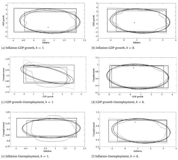
8.

For each of the three variables considered two-by-two,

Fig. 5plots 95% one-step-ahead bootstrap forecast ellip-soids and cubes for 2009Q4 (one step ahead) and 2011Q3 (eight steps ahead), together with the corresponding re-gions obtained under the assumption of Gaussian errors.

Fig. 5also plots the HDRs and the Bonferroni cubes which have been modified to take into account the correlations between the variables. In each case, the corresponding ob-served out-of-sample values are displayed by a dot. First, we can see that the Gaussian and bootstrap ellipsoids are rather similar, with the exception of the one-step-ahead GDP growth-unemployment ellipsoids, in which case the bootstrap is larger than that obtained under the assump-tion of Gaussianity. Also note that, whenh

=

1, the HDRs suggest non-elliptical densities, but whenh

=

8, HDRs are closer to the corresponding ellipsoids, suggesting that the Gaussianity may be plausible as the forecast horizon increases. Second, with respect to the Bonferroni cubes, note that the Gaussian cubes are much smaller than those obtained using the forward bootstrap procedure. Finally, when looking at the modified Bonferroni cubes, we can observe that, whenh

=

1, they only differ from the cor-responding original cube in the case of the GDP growth-unemployment region. It is worth mentioning that, when looking at whether or not the regions contain the true observations, we observe that all regions contain them

whenh

=

8. However, whenh

=

1, the GDP

growth-unemployment observation falls outside the Gaussian regions, but is close to the boundary of the bootstrap ellip-soid and cube, though clearly within the bounds of modi-fied Bonferroni cube.

Finally, we compare the empirical coverages obtained when constructing the forecast densities assuming Gaus-sian errors with and without parameter uncertainty and when implementing the backward and forward bootstrap procedures with the bias and lag-order corrections. For this purpose, we carry out a rolling window estimation with

T

=

100 observations, starting with data from 1948Q1