Institute for Empirical Research in Economics
University of Zurich
Working Paper Series
ISSN 1424-0459
Working Paper No. 245
Control of Generalized Error Rates in Multiple Testing
Joseph P. Romano and Michael Wolf
May 2005
Control of Generalized Error Rates in Multiple Testing
Joseph P. Romano∗ Department of Statistics Stanford University Stanford, CA 94305 U.S.AE-mail: romano@stanf ord.edu
Michael Wolf
Institute for Empirical Research in Economics University of Zurich
CH-8006 Zurich Switzerland
E-mail: [email protected]
May 18, 2005
Abstract
Consider the problem of testing s hypotheses simultaneously. The usual approach to dealing with the multiplicity problem is to restrict attention to procedures that control the probability of even one false rejection, the familiar familywise error rate (FWER). In many applications, particularly ifsis large, one might be willing to tolerate more than one false rejection if the number of such cases is controlled, thereby increasing the ability of the procedure to reject false null hypotheses One possibility is to replace control of the FWER by control of the probability of k or more false rejections, which is called the k-FWER. We derive both single-step and stepdown procedures that control the k-FWER in finite samples or asymptotically, depending on the situation. Lehmann and Romano (2005a) derive some exact methods for this purpose, which apply wheneverp-values are available for individual tests; no assumptions are made on the joint dependence of thep-values. In contrast, we construct methods that implicitly take into account the dependence structure of the individual test statistics in order to further increase the ability to detect false null hypotheses. We also consider the false discovery proportion (FDP) defined as the number of false rejections divided by the total number of rejections (and defined to be 0 if there are no rejections). The false discovery rate proposed by Benjamini and Hochberg (1995) controlsE(FDP). Here, the goal is to construct methods which satisfy, for a givenγandα,
P{FDP> γ} ≤α, at least asymptotically.
KEY WORDS: Bootstrap, False Discovery Proportion, False Discovery Rate,
Generalized Familywise Error Rates, Multiple Testing, Stepdown Procedure.
1
Introduction
The main goal of this paper is to show how computer-intensive methods can be used to con-struct asymptotically valid tests of multiple hypotheses under very weak conditions. In par-ticular, we construct computationally feasible methods which provide control (at least asymp-totically) of some generalized notions of the familywise error rate. However, the theory also applies to exact finite sample control in some situations.
Consider the problem of testing hypotheses H1, . . . , Hs. A classical approach to dealing
with the multiplicity problem is to restrict attention to procedures that control the probability of one or more false rejections, which is called the familywise error rate (FWER). Here the term “family” refers to the collection of hypothesesH1, . . . , Hsthat is being considered for joint
testing. For a given family, control of the FWER at (joint) level α requires that FWER ≤α
for all possible distributions of the data considered in the model, and therefore for all possible constellations of true and false hypotheses. A broad treatment of methods that control the FWER is given in Hochberg and Tamhane (1987).
Of course, safeguards against false rejections are not the only concern of multiple testing procedures. Corresponding to the power of a single test one must also consider the ability of a
procedure to detect departures from the null hypotheses. When the number of testssis large,
such as in genomics studies, control of the FWER at conventional levels becomes so stringent that individual departures from the null hypotheses have little chance of being detected. For this reason, we shall consider alternatives to the FWER that control false rejections less severely so that better power can be obtained.
First, we shall consider the k-FWER, the probability of rejecting at least k true null
hypotheses. Such an error rate with k > 1 is appropriate when one is willing to tolerate a
given number of false rejections. More formally, suppose dataX is available from some model
P ∈Ω. A general hypothesis H can be viewed as a subset ω of Ω. For testing Hi : P ∈ ωi,
i = 1, . . . , s, let I(P) denote the set of true null hypotheses when P is the true probability
distribution; that is,i∈I(P) if and only ifP ∈ωi. Then, the k-FWER, which depends onP
is defined to be
k-FWER =k-FWERP =P{reject at leastk hypothesesHi:i∈I(P)} . (1)
Control of thek-FWER requires that k-FWER ≤α for all P; that is,
k-FWERP ≤α for allP . (2)
Evidently, the casek= 1 reduces to control of the usual FWER.
We will also consider control of the false discovery proportion (FDP), defined as the total
number of false rejections divided by the total number of rejections (and equal to 0 if there
are no rejections). Given a user specified valueγ ∈[0,1), the measure of error control we wish
to control isP{FDP> γ}; thus, we wish to construct methods satisfying
We will derive methods where this is (at least asymptotically) bounded byα. Evidently, control
of the FDP with γ= 0 reduces to the usual FWER. Control of the false discovery rate (FDR)
requires thatE(FDP)≤α.
Recently, there have been a number of methods that control generalized error rates which are less stringent than the FWER. A prominent such technique is the FDR controlling method of Benjamini and Hochberg (1995). Additional methods that control the FDR are given in Benjamini and Yekutieli (2001) and Sarkar (2002). Genovese and Wasserman (2004) study asymptotic procedures that control the FDP (and the FDR) in the framework of a random effects mixture model. These ideas are extended in Perone Pacifico et al. (2004), where in the context of random fields, the number of null hypotheses is uncountable. Korn et al. (2004)
provide methods that control both thek-FWER and FDP; they provide some justification for
their methods, but they are limited to a multivariate permutation model. Alternative methods
of control of thek-FWER and FDP are given in van der Laan et al. (2004); they include both
finite sample and asymptotic results. Like the present work, their work attempts to capture the dependence between the tests with the goal of improved ability to detect false hypotheses; comparisons between the methods will be made later; see Section 5.
Some existing methods that control the k-FWER and FDP are we now briefly reviewed.
Suppose thatp-values ˆp1, . . . ,pˆs are available for testing H1, . . . , Hs. Formally, for ˆpi to be a
p-value, it is required that, for all u∈[0,1] and all P ∈ωi,
P{pˆi≤u} ≤u . (4)
Then, for any fixed k, the procedure that rejects Hi if ˆpi ≤ kα/s controls the k-FWER at
level α, and can be viewed as a generalization of the Bonferroni procedure which uses k= 1;
see Lehmann and Romano (2005a). It is an example of a single-step procedure, meaning any
null hypothesis is rejected if its correspondingp-value is less than or equal to a common cutoff
value.
Improvements are possible by considering a class of stepdown procedures, which we now
describe. Order thep-values by
ˆ
p(1) ≤pˆ(2) ≤ · · · ≤pˆ(s) ,
and letH(1), . . . , H(s) denote the corresponding hypotheses. Let
α1 ≤α2 ≤ · · · ≤αs (5)
be constants. If ˆp(1)> α1, reject no null hypotheses. Otherwise, if
ˆ
p(1)≤α1, . . . ,pˆ(r) ≤αr , (6) reject hypothesesH(1), . . . , H(r) where the largestr satisfying (6) is used. That is, a stepdown
procedure starts with the most significant p-value and continues rejecting hypotheses as a
remaining p-value is deemed “small”, where “small” is determined by the critical valueαj at
levelα. For generalk, consider the following generalized Holm stepdown procedure described in (6), where now we specifically set
αj = kα s j≤k kα s+k−j j > k (7)
Of course, theαj depend onsand k, but we suppress this dependence in the notation. Then,
the stepdown method described in (6) withαj given by (7) controls thek-FWER; that is, (2)
holds; see Hommel and Hoffman (1987) and Lehmann and Romano (2005a).
Turning to FDP control, Lehmann and Romano (2005a) reasoned as follows. To develop
a stepdown procedure satisfying (3), let F denote the number of false rejections. At step j,
having rejected j−1 hypotheses, we want to guarantee F/j ≤γ, i.e. F ≤ $γj%, where$x% is
the greatest integer ≤x. So, if k=$γj%+ 1, then F ≥k should have probability no greater
than α; that is, we must control the number of false rejections to be ≤k. Therefore, we use
the stepdown constant αj with this choice ofk(which now depends on j); that is,
αj =
($γj%+ 1)α
s+$γj%+ 1−j . (8)
Under certain dependence assumptions on the p-values, this method satisfies (3). Similar
methods that hold under no dependence assumptions are developed in Lehmann and Romano (2005a), Romano and Shaikh (2004) and Romano and Shaikh (2005).
In general, these generalized Holm type of methods assume a least favorable joint
distribu-tion for the p-values. In contrast, here we implicitly try to estimate the joint distribution of
p-values with the hopes of greater ability to detect false hypotheses.
In Section 2, we discuss stepdown methods that control the k-FWER in finite samples.
Such methods proceed stepwise by testing intersection hypotheses at each step. Using a sim-ple monotonicity condition for critical values, it is shown how computationally feasible (but possibly computer-intensive) methods can be constructed.
For any K ⊂ {1, . . . , s}, let HK denote the hypothesis that all Hi with i ∈ K are true.
The closure method of Marcus et al. (1976) allows one to construct methods that control the
FWER if one knows how to test each intersection hypothesisHK. Indeed, this method can be
generalized to control thek-FWER; see Appendix A. However, in general, this might require
the construction of nearly 2s tests. The constructions studied here only require a much lower
order number of tests; for example, the number of such tests is of order s in Algorithm 2.2.
In fact, the monotonicity assumptions we invoke can be viewed as justification to achieve this much lower order. (In some cases, shortcuts to applying the closure method are known. For example, Westfall et al. (2001) show how to apply closure to Fisher combination tests with only s2 evaluations.)
In general, we suppose that rejection of Hi is based on large values of a test statistic Tn,i.
(To be consistent with later notation, the n is used for asymptotic purposes and typically
refers to sample size.) Of course, if a p-value ˆpi is available for testing Hi, one possibility is to take Tn,i=−pˆi. Then, we restrict attention to tests that reject an intersection hypothesis
HK when the kth largest of the test statistics {Tn,i:i∈K} is large. In some problems where a monotonicity condition holds (distinct from the monotonicity assumption here), Lehmann
et al. (2005), for the particular case ofk= 1, show that such stepwise procedures are optimal
in a maximin sense. In other situations, it may be better to consider other test statistics that combine the individual test statistics in a more powerful way. A related issue is one of balance; see Remark 3.5. At this time, our primary goal is to show how stepdown procedures can be
constructed quite generally that control thek-FWER and FDP under minimal conditions; in
particular, we do not have to assume the subset pivotality condition of Westfall and Young (1993, page 42).
In Section 2, we show that, if we estimate critical values that have a monotonicity prop-erty, then the basic problem of constructing a valid multiple test procedure that controls the
k-FWER can essentially be reduced to the problem of sequentially constructing critical values
for (at most order s) single tests that control the usual Type 1 error. In particular, if finite
sample methods which offer control of the Type 1 error are available for each of the
individ-ual tests, then this will immediately translate into control of thek-FWER. For example, this
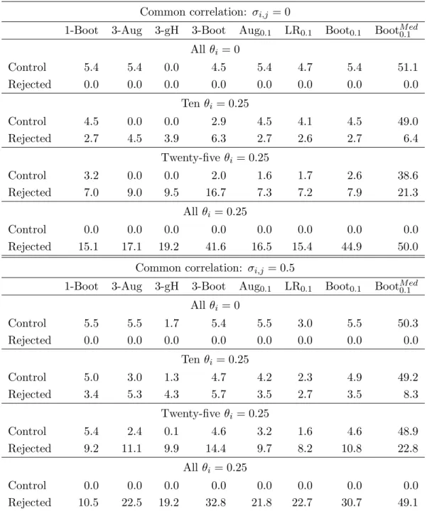
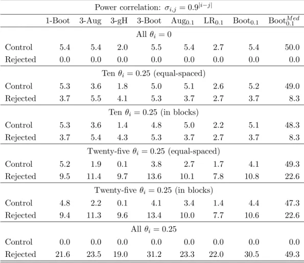
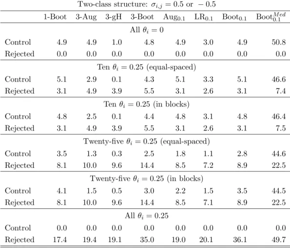
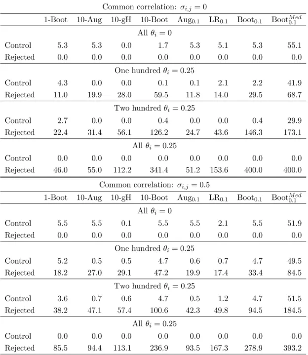
allows us to directly apply what we know about tests based on permutation and randomiza-tion distriburandomiza-tions. Alternatively, we can apply bootstrap and subsampling methods to achieve asymptotic control, as described in Section 3. Results for control of the FDP are obtained in Section 4. Comparisons with augmentation procedures are discussed in Section 5. In Section 6, we present a simulation study to examine the finite sample performance of some of the methods we suggest. All proofs are collected in an appendix.
2
Basic Results for Control of the
k-FWER
Suppose data X is generated from some unknown probability distributionP. In anticipation
of asymptotic results, we may write X = X(n), where n typically refers to the sample size.
A model assumes that P belongs to a certain family of probability distributions Ω, though we
make no rigid requirements for Ω. Indeed, Ω may be a nonparametric model, a parametric model, or a semiparametric model.
Consider the problem of simultaneously testing a hypothesisHi againstHi#, fori= 1, . . . , s.
Of course, a hypothesisHican be viewed as a subset,ωi, of Ω, in which case the hypothesisHi
is equivalent toP ∈ωi andHi# is equivalent toP /∈ωi. For any subset K⊂ {1, . . . , s}, define
HK =
$
i∈K
Hi
to be theintersection hypothesis thatP ∈%
i∈Kωi.
Suppose that a test of the individual hypothesisHiis based on a test statisticTn,i, with large
values indicating evidence againstHi. For an individual hypothesis, numerous approaches exist
to approximate a critical value, such as those based on classical likelihood theory, bootstrap tests, Edgeworth expansions, permutation tests, etc.. The main problem addressed in the present work is to construct procedures that control generalized familywise error rates, the
Some further notation is required. Suppose {yi : i ∈ K} is a collection of real numbers
indexed by a finite set K having |K| elements. Then, for k ≤ |K|, the k-max(yi :i ∈ K) is
used to denote the kth largest value of the yi with i∈ K. So, if the elements yi, i∈ K, are
ordered as
y(1) ≤ · · · ≤y(|K|) ,
then
k-max(yi :i∈K) =y(|K|−k+1) .
2.1 Single-step Control of the k-FWER
Throughout this section, kis fixed. First, we briefly discuss a single-step approach to control
of thek-FWER, since it serves as a building block for the more powerful stepdown procedures
considered later, much in the same way the Bonferroni method is a building block for the more powerful Holm method. For any subsetK ⊂ {1, . . . , s}, letcn,K(α, k, P) denote anα-quantile of the distribution of k-max(Tn,i:i∈K) underP. Concretely,
cn,K(α, k, P) = inf{x: P{k-max(Tn,i:i∈K)≤x} ≥α} . (9)
(We use the subscriptn for asymptotic purposes later on, though the priority in this section
is to study nonasymptotic results.)
For testing the intersection hypothesis HK with K ⊂ {1, . . . , s}, it is only required to
approximate a critical value forP ∈%
i∈Kωi. Because there may be many suchP, we define
cn,K(1−α, k) = sup{cn,K(1−α, k, P) : P ∈
$
i∈K
ωi}. (10) (In order to definecn,K(α, k), we implicitly assumed%si=1ωi is not empty.)
Consider the idealized test that rejects any Hi for which Tn,i > cn,I(P)(1−α, k, P). This
is a single-step method in that each Tn,i is compared with a common cutoff. However, this
is an idealization because the critical valuecn,I(P)(1−α, k, P) is in general unknown. Such a fictional test clearly controls thek-FWER at levelαif the distribution ofk-max(Tn,i:i∈I(P)) is continuous underP; otherwise, we can still bound thek-FWER byα. Indeed, if|I(P)|< k, then there is nothing to prove; otherwise,
P{kor more false rejections}=P{k-max(Tn,i:i∈I(P))> cn,I(P)(1−α, k, P)} ≤α ,
with equality if the distribution ofk-max(Tn,i:i∈I(P)) is continuous underP. Unfortunately, the test is unavailable as the critical value is in general unknown.
One possible approach is to replace cn,I(P)(1−α, k, P) by cn,I(P)(1−α, k), but this still
depends on P through I(P). Since I(P) is unknown, a conservative approach would be to
assume all hypotheses are true and replace cn,I(P)(1 −α, k) by cn,A(1−α, k), where A =
{1, . . . , s}.
Unfortunately, in nonparametric problems, the sup in (10) may be formidable or impossible to calculate, and may be way too conservative anyway. Instead, another possibility is to
replace the critical valuecn,I(P)(1−α, k, P) by some estimate ˆcn,I(P)(1−α, k), which is at least
consistent or conservative. In general, suppose ˆcn,K(1−α, k) represents an approximation or
estimate of the 1−α quantile of the distribution of k-max(Tn,i : i∈K), at least valid when
Hi is true fori∈K. Bootstrap and subsampling methods offer viable general approaches, and
will be used later. Such a single-step approach using thek-max statistic was also discussed in
Dudoit et al. (2004). (Rather than formalizing the required conditions for consistency right now, we will later give explicit conditions for more powerful stepdown methods.) A single-step
approach would then be to replaceK byA={1, . . . , s}. To give concrete representations, we
offer two examples.
Example 2.1 (Multivariate Normal Mean) Suppose (X1, . . . , Xs) is multivariate normal
with unknown meanµ= (µ1, . . . , µs) and known covariance matrix Σ having (i, j) component
σi,j. Consider testingHi:µi ≤0 versusµi >0. LetTn,i=Xi/√σi,i, since the test that rejects for large Xi/√σi,i is U M P for testing Hi. For |K| ≥k,cn,K(1−α, k) is the 1−α quantile of
the distribution ofk-max(Tn,i : i∈K) when µ= 0. A single-step approach would reject any
Tn,ithat exceedscn,A(1−α, k), whereA={1, . . . , s}. Since
cn,A(1−α, k)≥cn,I(P)(1−α, k)≥cn,I(P)(1−α, k, P) ,
this procedure clearly controls the k-FWER. Of course, it is strictly more powerful than a
Bonferroni procedure, since it accounts for the dependence between the test statistics.
In the special case when k= 1 and σi,i =σ2 is independent of i and σi,j has the product
structureσi,j =λiλj, then Appendix 3 of Hochberg and Tamhane (1987, page 374) reduces the
problem of determining the distribution of the maximum of a multivariate normal vector to a
univariate integral. For general k or general Σ, one can resort to simulation to approximate
the critical values.
Outside some parametric models or models where permutation tests apply, exact critical values are usually not available. We now offer a concrete approach based on the bootstrap. The theory of asymptotic control will follow from results for the more powerful stepdown method which we develop later.
Example 2.2 Suppose Hi is concerned with a test of a parameter; that is, Hi is specified by {P : θi(P) ≤ 0} for some real-valued parameter θi. Let ˆθn,i be an estimate of θi. Also,
let Tn,i = τnθˆn,i for some nonnegative (nonrandom) sequence τn → ∞. The sequence τn is
introduced for asymptotic purposes so that a limiting distribution for τn[ˆθn,i−θi(P)] exists. In typical situations,τn=n1/2.
The bootstrap method relies on its ability to approximate the joint distribution of{τn[ˆθn,i−
θi(P)] : i∈K}, which we denote byJn,K(P).
For K ⊂ {1, . . . , s} with |K| ≥ k, let Ln,K(k, P) denote the distribution under P of
k-max(τn[ˆθn,i−θi(P)] : i∈K), with corresponding cumulative distribution functionLn,K(x, k, P)
and α-quantile
Let ˆQn be some estimate of P. For i.i.d. data, ˆQn is typically taken to be the empirical distribution, or possibly a smoothed version. For time series or data-dependent situations,
block bootstrap methods should be employed; see Lahiri (2003). LetA ={1, . . . , s}. Then, a
nominal 1−α level bootstrap joint confidence region for the subset of parameters{θi(P) : i∈
A} is given by {(θi : i∈A) : max i∈A τn[ˆθn,i−θi]≤bn,A(1−α,1, ˆ Qn)} (11) ={(θi : i∈A) :θi≥θˆn,i−τn−1bn,A(1−α,1,Qˆn)}.
A value of 0 for θi(P) falls outside the region if and only ifτnθˆn,i> bn,A(1−α,1,Qˆn). By the usual duality of confidence sets and hypothesis tests, this suggests the use of the critical value
ˆ
cn,A(1−α,1) =bn,A(1−α,1,Qˆn) , (12)
to control the familywise error rate (i.e. thek-FWER withk= 1) at least if the bootstrap is a
valid asymptotic approach for joint confidence region construction. Since here, we require con-trol of thek-FWER, we merely replace the max in (11) with thek-max and bn,A(1−α,1,Qˆn) withbn,A(1−α, k,Qˆn). Such a generalized joint confidence region should asymptotically
con-tain all true parameter values except for possibly at most k−1 of them, with probability
(asymptotically) at least 1−α. Thus, the bootstrap critical value we use will be
ˆ
cn,A(1−α, k) =bn,A(1−α, k,Qˆn) . (13) Asymptotic control of this single-step bootstrap method will follow from later results on the more powerful stepdown bootstrap method of Section 3.1.
2.2 Stepdown Methods That Control the k-FWER Let
Tn,r1 ≥Tn,r2 ≥ · · · ≥Tn,rs (14)
denote the observed ordered test statistics, and let Hr1, Hr2, . . . , Hrs be the corresponding
hypotheses.
Stepdown methods begin by first applying a single-step method, but then additional hy-potheses may be rejected after this first stage by proceeding in a stepwise fashion, which we now describe. Begin by testing the joint null (intersection) hypothesisH{1,...,s} that all hypotheses
are true. This hypothesis is rejected if Tn,r1 is deemed large, in which case Hr1 is rejected.
Here, the meaning of large is determined by some critical value ˆcn,A(1−α, k), which is designed to offer single-step control when testing the intersection hypothesis HA with A = {1, . . . , s}. If it is not large, accept all hypotheses; otherwise, reject the hypothesis corresponding to the largest test statistic. Once a hypothesis is rejected, the next most significant hypothesis cor-responding to the next largest test statistic is considered, and so on. At any stage, one tests
appropriate intersection hypotheses HK. Suppose that critical constants ˆcn,K(1−α, k) are
available from our statistical tool chest, which we might contemplate for use as a single step
procedure for testing HK. The critical constants ˆcn,K(1−α, k) may be fixed or random, but
Algorithm 2.1 (Generic Stepdown Method For Control of the k-FWER)
1. Let A1 ={1, . . . , s}. If max(Tn,i :i∈A1) ≤ˆcn,A1(1−α, k), then accept all hypotheses and stop; otherwise, reject anyHi for which Tn,i>ˆcn,A1(1−α, k) and continue.
2. Let R2 be the indices i of hypotheses Hi previously rejected, and let A2 be the indices
of the the remaining hypotheses. If|R2|< k, then stop. Otherwise, let
ˆ
dn,A2(1−α, k) = max{ˆcn,K(1−α, k) :K =A2∪I, I ⊂R2, |I|=k−1}.
Then, reject anyTn,iwithi∈A2 satisfying Tn,i>dˆn,A2(1−α, k). If there are no further rejections, stop.
.. .
j. Let Rj be the indices i of hypotheses Hi previously rejected, and let Aj be the indices
of the remaining hypotheses. Let ˆ
dn,Aj(1−α, k) = max{cˆn,K(1−α, k) :K =Aj∪I, I ⊂Rj, |I|=k−1} .
Then, reject anyTn,i withi∈Aj satisfyingTn,i>dˆn,Aj(1−α, k). If there are no further
rejections, stop. ..
.
And so on.
Note that, in the case k = 1, once a hypothesis is removed, it no longer enters into the
algorithm. However, for k > 1, the algorithm becomes slightly more complex. The reason
is that, for control of the k-FWER, we must acknowledge that when we consider a set of
hypotheses not previously rejected, we may have gotten to that stage in the algorithm by
rejecting true null hypotheses, but hopefully at most k−1 of them. Since we do not know
which of the hypotheses rejected thus far are true or false, we must maximize over subsets
including some of those rejected, but at mostk−1 among the previously rejected ones. Note
that, in the case k = 1, no previously rejected hypotheses need be considered any further
in the determination of whether more hypotheses will be rejected. Thus, the case k = 1, as
considered in Romano and Wolf (2005a) is particularly simple, especially from a computational
point of view. Our main point will be that, if we can control thek-FWER at any stage of the
algorithm, then the stepdown test will control thek-FWER.
Remark 2.1 (Modified Generic Stepdown Method For Control of the k-FWER)
The following modification of Algorithm 2.1 has the exact same properties in terms ofk-FWER
control but potentially rejects more false hypotheses: If Algorithm 2.1 rejects at least k−1
hypotheses, reject the same hypotheses. Otherwise, rejectHr1, . . . , Hrk−1. In other words, the
promote this approach, as it can lead to counterintuitive results. Take the case where individ-ualp-values are available and the test statistics are of the formTn,i= 1−pˆi. For anyk≥2 one would then always rejectHr1 even if ˆpr1 = 0.5, say. On the other hand, for certain applications this modified algorithm may be preferred.
In order to prove such an algorithm controls the k-FWER for suitable choice of critical
values ˆcn,K(1−α, k), we assume monotonicity of the estimated critical values; that is, for any
K ⊃I(P),
ˆ
cn,K(1−α, k)≥cˆn,I(P)(1−α, k) . (15)
Ideally, we would also like the following to hold: if ˆcn,K(1−α, k) is used to test the intersection
hypothesis HK, then the chance of k or more false rejections is bounded above by α when
K =I(P); that is,
P{k-max(Tn,i: i∈I(P))>cˆn,I(P)(1−α, k)} ≤α . (16)
Under the monotonicity assumption (15), we will show the basic inequality thatk-FWERP is
bounded above by left side of (16). This will then show that, if we can construct monotone
critical values such that each intersection test controls the k-FWER, then the stepdown
pro-cedure controls the k-FWER. Thus, the construction of a stepdown procedure is effectively
reduced to construction of single tests, as long as the monotonicity assumption holds. Also, note the monotonicity assumption for the critical values can be made to hold by construction
and can be enforced, that is, it does not depend on the unknownP.
Theorem 2.1 LetP denote the true distribution generating the data. Consider Algorithm 2.1 with critical valuescˆn,K(1−α, k) satisfying (15).
(i) Then,
k-FWERP ≤P{k-max(Tn,i: i∈I(P))>cˆn,I(P)(1−α, k)} . (17)
(ii) Therefore, if the critical values also satisfy (16), then k-FWERP ≤α.
The monotonicity assumption (15) cannot be removed, as shown in Example 2.1 of Romano
and Wolf (2005a), in the case k = 1, and an analogous construction works for general k.
Fortunately, the general resampling constructions we describe later will inherently satisfy (15). As a corollary, suppose we consider the nonrandom choice of critical values
ˆ
cn,K(1−α, k) =cn,K(1−α, k)
defined in (10). Assume the following monotonicity assumption: forK ⊃I(P),
cn,K(1−α, k)≥cn,I(P)(1−α, k) . (18)
The condition (18) can be expected to hold in many situations because the left hand side
is based on computing the 1−α quantile of thekth largest of |K| variables, while the right
hand side is based on the kth largest of |I(P)| ≤ |K| variables (though one must be careful
and realize that the quantiles are computed under possibly different P, which is why some
Corollary 2.1 Let P denote the true distribution generating the data. Assume%s
i=1ωi is not
empty.
(i) Assume (18). Consider Algorithm 2.1 with ˆcn,K(1 −α, k) = cn,K(1 −α, k). Then,
k-FWERP ≤α.
(ii) Strong control persists if, in Algorithm 2.1, the critical constants ˆcn,K(1−α, k) are
re-placed by dn,K(1−α, k) which satisfy
dn,K(1−α, k)≥cn,K(1−α, k) . (19)
(iii) Moreover, the condition (18) may then be removed if the dn,K(1−α, k) satisfy
dn,K(1−α, k)≥dn,I(P)(1−α, k) (20)
for anyK ⊃I(P).
Example 2.3 (Multivariate Normal Mean, continuation of Example 2.1) Recall that (X1, . . . , Xs) is multivariate normal with unknown mean µ= (µ1, . . . , µs) and known covari-ance matrix Σ having (i, j) component σi,j. Consider testingHi :µi ≤ 0 versus µi >0. Let
Tn,i=Xi/√σi,i. To apply Corollary 2.1, assume that|I(P)| ≥kor there is nothing to prove. Letcn,K(1−α, k) be the 1−α quantile of the distribution ofk-max(Tn,i: i∈K) whenµ= 0. Since
k-max(Tn,i: i∈I)≤k-max(Tn,i: i∈K)
whenever I ⊂K, the monotonicity requirement (18) is satisfied. Moreover, the resulting test
procedure rejects at least as many hypotheses as the generalized Holm procedure, as it accounts for the dependence of the test statistics.
Example 2.4 (One-way Layout) Suppose fori= 1, . . . , sandj= 1, . . . , ni,Xi,j =µi+(i,j, where the (i,j are i.i.d. N(0, σ2); the vector µ= (µ1, . . . , µs) andσ2 are unknown. Consider testing Hi :µi= 0 against µi-= 0. Let tn,i=√niX¯i,·/S, where
¯ Xi,·= 1 ni ni & j=1 Xi,j, S2= 1 ν s & i=1 ni & j=1 (Xi,j−X¯i,·)2 , and ν='
i(ni−1). UnderHi,tn,i has a t-distribution withν degrees of freedom. LetTn,i=
|tn,i|, and letcn,K(1−α, k) denote the 1−α quantile of the distribution ofk-max(Tn,i: i∈K)
when µ= 0 and σ= 1. Since, for |I| ≥k,
k-max(Tn,i: i∈I)≤k-max(Tn,i: i∈K) ,
whenever I ⊂K, the monotonicity requirement (18) follows. Note that the joint distribution
of (tn,1, . . . , tn,s) follows ans-variate multivariate t-distribution withν degrees of freedom; see Hochberg and Tamhane (1987, pp. 374–375).
The previous examples are parametric in nature and the null distributions for testing inter-section hypotheses do not depend on nuisance parameters. However, we will see that a valid stepdown approach can apply to semiparametric and nonparametric problems if we can con-struct single step tests of intersection hypotheses whose critical values satisfy the monotonicity requirement. Our main goal will be to apply resampling methods that can implicitly account for the dependence structure of the test statistics. However, we first observe that the fact that
the generalized Holm procedure controls the k-FWER follows from Corollary 2.1.
Example 2.5 (Generalized Holm procedure) The stepdown procedure described by (6)
with critical values given by (7) controls thek-FWER. This follows from Theorem 2.1 and the
fact that, when testing |K| hypotheses, the single-step procedure that rejects any hypothesis
for which its correspondingp-value is≤kα/|K|controls thek-FWER; see Theorem 2.1 (i) of
Lehmann and Romano (2005). Note that the critical valueskα/|K|are monotone in |K|.
Remark 2.2 In general, the critical values used in Corollary 2.1(i) are the smallest constants
possible without violating the k-FWER. As a simple example, suppose Xi, i = 1, . . . , s, are
independentN(θi,1), with the θi varying freely. The null hypothesis Hi specifies θi ≤0 and
Tn,i = Xi. Then, cn,K(1−α, k) is the 1−α quantile of k-max(Z1, . . . , Z|K|), where the Zi
are i.i.d. N(0,1). Suppose c is a constant and c < cn,K(1−α, k) for some subset K with
|K∩I(P)| ≥k. As θi → ∞ fori /∈K and θi = 0 fori∈K, the probability ofk or more false rejections tends to
P{k-max(Xi :i∈K)> c}> P{k-max(Xi:i∈K)> cn,K(1−α, k)}=α .
Thus, the sup over P of the probability (underP) that Algorithm 2.1 rejects anyi∈I(P)
is equal to α. It then follows that the critical values cannot be made smaller, in hopes of
increasing the ability to detect false hypotheses, without violating the strong control of the
k-FWER. However, the above only applies to nonrandom critical values and does not negate
the possibility that critical values can be estimated, and therefore be random. That is, if
we replace cn,K(1−α, k) by some estimate ˆcn,K(1−α, k), it can sometimes be smaller than
cn,K(1−α, k) as long as it is not with probability one. Of course, it is typically the case that critical values need to be estimated, such as by permutation tests, resampling, bootstrap and subsampling methods, and these will be considered in the later sections.
In the examples considered so far, the application of the Generic Stepdown Method was not highly computational because the critical values essentially only depended on the number of hypotheses being tested at any stage. When this is not the case, the procedure becomes more computational. However, we will also consider the following more streamlined algorithm. The basic idea is that at any stage, when testing whether or not to include further rejections,
we need only look at the hypotheses not previously rejected together with thek−1 hypotheses
that are least significant among those previously rejected. So, we avoid maximizing over all
subsets of sizek−1 of previously rejected hypotheses and just look at the most “recent”k−1
rejections. The arguments for such a procedure will be asymptotic. The algorithm looks like this.
Algorithm 2.2 (Streamlined Stepdown Method For Control of the k-FWER)
1. Let A1 ={1, . . . , s}. If max(Tn,i :i∈A1) ≤ˆcn,A1(1−α, k), then accept all hypotheses and stop; otherwise, reject anyHi for which Tn,i>ˆcn,A1(1−α, k) and continue.
2. Let R2 be the indices i of hypotheses Hi previously rejected, and let A2 be the indices
of the remaining hypotheses. IfR2< k, then stop. Otherwise, letK be the union ofA2
together with thek−1 least significant hypotheses among those previously rejected, so
K ={r(|R2|−k+2), r(|R2|−k+3), . . . , r(s)} .
Set
˜
dn,A2(1−α, k) = ˆcn,K(1−α, k) .
Then, reject anyTn,iwithi∈A2 satisfying Tn,i>d˜n,A2(1−α, k). If there are no further rejections, stop.
.. .
j. Let Rj be the indices i of hypotheses Hi previously rejected, and let Aj be the indices
of the remaining hypotheses. Let K be the union of Aj together with the k−1 least
significant hypotheses among those previously rejected, so
K ={r(|Rj|−k+2), r(|Rj|−k+1), . . . , r(s)} .
Let
˜
dn,Aj(1−α, k) = ˆcn,K(1−α, k) .
Then, reject anyTn,i withi∈Aj satisfyingTn,i>d˜n,Aj(1−α, k). If there are no further
rejections, stop. ..
.
And so on.
2.3 Permutation and Randomization Tests
We now show how Theorem 2.1 can be applied to permutation and randomization tests. First, we review a general construction of a randomization test in the context of a single test, because the key result of Theorem 2.1 is that the general problem of constructing valid stepdown tests can be reduced to the construction of tests of intersection hypotheses, as long as we can verify the monotonicity requirement. Our setup is framed in terms of a population model, but similar results are possible in terms of a randomization model (as in Section 3.1.7 of Westfall and Young, 1993).
Based on data X taking values in a sample space X, it is desired to test the null
ω of distributions. Let G be a finite group of transformations g of X onto itself. The
fol-lowing assumption, which we will call therandomization hypothesis, allows for a general test
construction.
The Randomization Hypothesis The null hypothesis implies that the distribution ofX is
invariant under the transformations inG; that is, for every g inG,gX and X have the same
distribution wheneverX has distribution P inω.
As an example, consider testing the equality of distributions based on two independent samples (Y1, . . . , Ym) and (Z1, . . . , Zn). Under the null hypothesis that the samples are gener-ated from the same probability law, the observations can be permuted or assigned at random to either of the two groups, and the distribution of the permuted samples is the same as the dis-tribution of the original samples. In this example, and more generally when the randomization hypothesis holds, the following construction of a randomization test applies.
Let T(X) be any real-valued test statistic for testing H. Suppose the group G has M
elements. Given X=x, let
T(1)(x)≤T(2)(x)≤ · · · ≤T(M)(x)
be the values ofT(gx) asgvaries inG, ordered from smallest to largest. Fix a nominal levelα, 0< α <1, and let m be defined by
m=M− $M α%, (21)
where $M α% denotes the largest integer less than or equal to M α. Let M+(x) and M0(x)
be the number of values T(j)(x) (j = 1, . . . , M) which are greater than T(m)(x) and equal to
T(m)(x), respectively. Set
a(x) = M α−M
+(x)
M0(x) .
Define the randomization test function φ(X) to be equal to 1, a(X), or 0 according to
whether T(X)> T(m)(X),T(X) =T(m)(X), or T(X)< T(m)(X), respectively.
Under the randomization hypothesis, Hoeffding (1952) shows this construction produces a test that is exact levelα, and this result is true foranychoice of test statisticT. Note that this
test is possibly a randomized test ifM αis not an integer of there are ties in the ordered values.
Alternatively, if one prefers not to randomize, the slightly conservative butnonrandomizedtest
that rejects if T(X)> Tm(X) is level α.
In general, one can define a p-value ˆpof a randomization test by
ˆ p= 1 M & g I{T(gX)≥T(X)}. (22) It is easily shown that ˆp satisfies, under the null hypothesis,
P{pˆ≤u} ≤u for all 0≤u≤1 . (23)
We now return to the multiple testing problem. AssumeGK is a group of transformations
for which the randomization hypothesis holds forHK. Then, if we wish to control thek-FWER,
we can apply the above construction to test the single intersection hypothesis HK based on
the test statistic
Tn,K =k-max(Tn,i: i∈K) (24)
and reject HK when
Tn,K(X)> T(|
GK|−%|GK|α&)
n,K (X) .
If it is also the case thatGK =G, so that the sameGapplies to all intersection hypotheses,
then we can verify the monotonicity assumption for the critical values. Setmα =|G|−$|G|α%.
Then, for anyg∈Gand I ⊂K,
k-max(Tn,i(gX) : i∈K)≥k-max(Tn,i(gX) : i∈I) , (25)
and so asgvaries, themαth largest value of the left side of (25) is at least as large as themαth largest value of the right side.
Consequently, the critical values ˆ
cn,K(1−α, k) =Tn,K(mα) , (26)
satisfy the monotonicity requirement of Theorem 2.1. Moreover, by the general randomization construction of a single test, the test that rejectsHK whenTn,K ≥Tn,K(mα)is levelα. Therefore, the following is true.
Corollary 2.2 Suppose the randomization hypothesis holds for a group G when testing any intersection hypothesis HK. Then, the stepdown method with critical values given by (26)
controls the k-FWER at levelα.
Remark 2.3 BecauseG may be large, one may resort to a stochastic approximation to
con-struct the randomization test, by randomly sampling transformations g from G. The results
are valid in this case; see Romano and Wolf (2005) who considered the case k = 1, but the
results generalize.
In the above corollary, we have worked with the randomization construction using nonran-domized tests. A similar result would hold if we permit randomization.
Example 2.6 (Two Sample Problem With k Variables) SupposeY1,· · · , YnY is a
sam-ple of nY independent observations from a probability distribution PY and Z1,· · · , ZnZ is a
sample ofnZobservations fromPZ. Here, PY andPZ are probability distributions onRs, with
ith components denotedPY,i andPZ,i, respectively. The hypothesisHj asserts PY,i=PZ,iand we wish to test thesekhypotheses based on X= (Y1,· · · , YnY, Z1,· · ·, ZnZ). Also, let Yj,i
de-note theith component ofYj andZj,i denote theith component ofZj. As in Troendle (1995),
we assume a semiparametric model. In particular, assumePY andPZare governed by a family
of probability distributionsQθ indexed by θ= (θ1, . . . , θs)∈Rs (and assumed identifiable), so
the mean vector, though this assumption is not necessary. Now, Hi can be viewed as testing
θY,i =θZ,i. Note that the randomization construction does not need to assume knowledge of
the form of Q(just as a single two-sample permutation test in a shift model does not need to
know the form of the underlying distribution under the null hypothesis).
Letn=nY+nZ, and forx= (x1,· · · , xn)∈Rn, letgx∈Rnbe defined by (xπ(1),· · · , xπ(n)),
where (π(1),· · ·, π(n)) is a permutation of (1,2,· · · , n). Let G be the collection of all suchg
so that M = n!. Under the hypothesis PY =PZ, gX and X have the same distribution for
any g inG.
Unfortunately, this Gdoes not apply to any subsetK of the hypotheses, because gX and
X need not have the same distribution if only a subcollection of the hypotheses are true.
However, we just need a slight generalization to cover the example. Suppose that the test
statistic Tn,i used to test Hi only depends on theith components of the observations, namely
Yj,i,j= 1, . . . , nY andZj,i,j= 1, . . . , nZ; this is a weak assumption indeed. In fact, letXK be
the data set consisting of the the componentsYj,iandZj,iasivaries only inK. The simple but
important point here is that, for this reduced data set, the randomization hypothesis holds.
Specifically, under the null hypothesis θY,i = θZ,i for i ∈ K, XK and gXK have the same
distribution (though X and gX need not). Also, for any g ∈ G, Tn,i(gX) and Tn,i(X) have
the same distribution underHi, and similarly for anyK ⊂ {1, . . . , s},Tn,K(gX) and Tn,K(X)
have the same distribution underHK.
Then, because the same G applies in this manner for all K, the critical values from the
randomization test are monotone, just as in (25). Moreover, each intersection hypothesis can
be tested by an exact level α randomization test (since inference for HK is based only on
XK). Therefore, essentially the same argument leading to Corollary 2.2 applies. In particular,
even if we need to resort to approximate randomization tests at each stage, but as long as we
sample the same set of gj from G, the resulting procedure retains its finite sample property
of controlling thek-FWER. In contrast, Troendle (1995), discussing the special case ofk= 1,
concludes asymptotic control only. For general k, Korn et al. (2004) discuss finite sample
control of the k-FWER in the setting of this example
Example 2.7 (Semiparametric version of Example 2.3) Suppose, for j = 1, . . . , n, Xj are i.i.d. s-variate withXj = (Xj,1, . . . , Xj,s). It is assumedXj =µ+(j, whereµ= (µ1, . . . , µs)
and the (j are i.i.d. random vectors with s-variate distribution F. The distribution of F is
unknown, but greatly weakening the assumption of multivariate normality, it is assumed that
the distribution of F is symmetric in the sense that the distribution of (j is the same as that
of −(j. Consider testingH0 :µi= 0 against µi-= 0. Let tn,i=√nX¯n,i/Sn,i, where ¯ Xn,i= 1 n n & j=1 Xj,i, Sn,i2 = 1 n n & j=1 (Xj,i−X¯n,i)2 ;
also, set Tn,i = |tn,i|. To test the intersection hypothesis HK, consider the group GK of
2n transformations of the form
where theδi are either 1 or -1. These transformations apply to anyK, but as in the previous
example, the randomization hypothesis strictly speaking does not hold for testing HK.
How-ever, as in the previous example,Tn,K(X) andTn,K(gX) have the same distribution underHK
and the argument leading to Corollary 2.2 applies to yield exact finite sample control of the
k-FWER.
Remark 2.4 It is interesting to study the behavior of randomization and permutation pro-cedures if the model is such that the randomization hypothesis does not hold. For example,
in Example 2.7, we may be interested in testing Hj : µi = 0 even if Xj,i is not assumed
to have a symmetric distribution. Then, the randomization test construction of this section fails because the randomization hypothesis need not hold. However, since the randomization procedure has monotone critical values (as this is only a property of how the data is used), Theorem 2.1(i) applies. Therefore, one can again reduce the problem of studying control of the
k-FWER to that of controlling the level of a single intersection hypothesis. But the problem
of controlling the level of a single test when the randomization hypothesis fails is studied in Romano (1990) and so similar methods can be used here, with the hope of at least proving asymptotic control. Alternatively, the more general resampling approaches of Section 3 can be employed; the comparison of randomization and bootstrap tests is studied in Romano (1989) and it is shown they are often quite close, at least when the randomization hypothesis holds.
Example 2.8 (Comparison of Multiple Treatments with a Control) Consider the
one-way anova model. We are given s+ 1 independent samples, with the ith sample having ni
i.i.d. observationsXi,j,j = 1, . . . , ni. SupposeXi,j has distributionPi. The problem is to test
the hypotheses ofstreatments with a control; that is,Hi: Pi =Ps+1. (Alternatively, we can
test all pairs of distributions, but the issues are much the same, so we illustrate them with the
slightly easier setup.) Under the joint null hypothesis, we can randomly assign alln='s+1
i=1 ni
observations to any of the groups; that is, the groupGconsists of all permutations of the data.
However, if only a subset of the hypotheses are true, this group is not valid. A simple remedy is
to permute only within subsets; that is, to test any subset hypothesisHK, only consider those
permutations that permute observations within the samples Xi,j with i∈ K and the sample
Xs+1,j. Therefore, one computes a critical value ˆcn,K(1−α, k) by the randomization test with
the group GK of permutations within samples i∈K and i=s+ 1. Unfortunately, this does
not lead to monotonicity of critical values, and the previous results do not apply. But, we can apply the generalized closure method of the appendix, if one is willing to compute critical values for all subset hypotheses. On the other hand, this can be computationally prohibitive. Such issues are raised by Petrondas and Gabriel (1983) (although the problem was not framed in terms of a monotonicity requirement). Fortunately, the lack of monotonicity of critical values is only a concern if strict finite sample control is required; otherwise, computationally quicker bootstrap methods described in the next section apply to yield asymptotic control.
3
Asymptotic Results on
k-FWER Control
The main goal of this section is to show how Theorem 2.1 can be used to construct stepdown
procedures that asymptotically control thek-FWER under very weak assumptions. The use of
resampling techniques will be a key ingredient. The assumptions are identical to the weakest assumptions available for the contruction of asymptotically valid tests of a single hypothesis, which are used in many resampling schemes, and so one cannot expect to improve them without improving the now well-developed theory of resampling methods for testing a single hypothesis. The methods constructed will be based in Algorithm 2.1, and so many tests are constructed
in a stepwise fashion. However, a key feature is that the methods will only require one set of
resamples for all of the tests, whether they are bootstrap samples or subsamples.
In order to accomplish this, we will consider resampling schemes that do notobey the null
hypothesis constraints. Hypothesis test constructions that do obey the constraints imposed the null hypothesis, as discussed in Beran (1986) and Romano (1988), are based on the idea that the critical value should be obtained under the null hypothesis and so the resampling scheme should reflect the constraints of the null hypothesis. This idea is even advocated as a principle in Hall and Wilson (1991), and it is enforced throughout Westfall and Young (1993). While appealing, it is by no means the only approach toward inference in hypothesis testing. Indeed, the well-known explicit duality between tests and confidence intervals means that if you can construct good or valid confidence intervals, then you can construct good or valid tests, and conversely. For example, by resampling from the empirical distribution to construct a confidence interval for a single parameter, very desirable intervals can be constructed, which would then translate into desirable tests. The same holds for simultaneous confidence sets and multiple tests.
That is not to say that the approach of obeying the null constraints is less appealing. It is, however, often more difficult to apply, and it is unlikely that one resampling scheme obeying the constraints of all hypotheses would work in general in the multiple testing framework. An alternative approach would be to resample from a different distribution at each step, obeying the constraints of the null hypotheses imposed at each step. This approach would probably succeed in a fair amount of generality, but even so, two problems would remain. First, it may be difficult to determine the appropriate resampling sheme for testing each subset hypothesis. Second, even if one knew how to resample at each stage, there is increased computation. Our approach avoids these complications. In some problems, the subset pivotality condition of Westfall and Young (1993) holds, and so the same null distribution can be used at each step. However, this condition does not hold in general, as the following example shows.
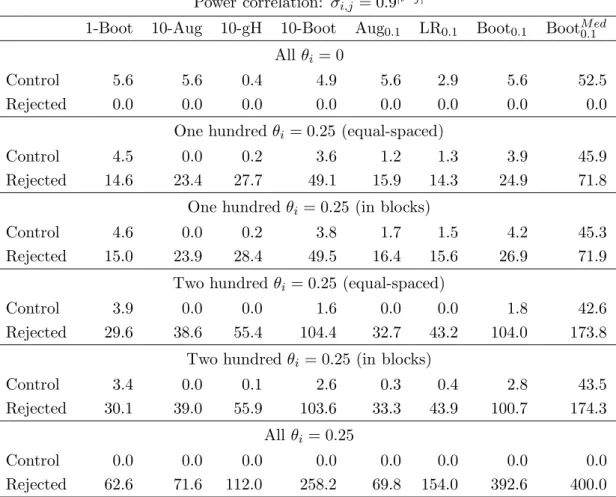
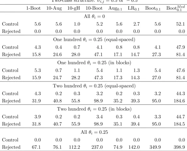
Example 3.1 (Testing Correlations) Let X1, . . . , Xn be i.i.d. random vectors in Rd, with
Xi= (Xi,1, . . . , Xi,d). AssumeE|Xi,j|2 <∞andV ar(Xi,j)>0. Then, the correlation between
X1,iand X1,j, namelyρi,j is well-defined. LetHi,j denote the hypothesis thatρi,j = 0, so that
the multiple testing problem consists in testing alls=(d
2
)
pairwise correlations. Also letTn,i,j
denote the ordinary sample correlation between variablesiand j. (Note that we are indexing
(1993), Example 2.2, p. 43, subset pivotality fails here. For example, using results of Aitken
(1969) and Aitken (1971), if d = s = 3, H1,2 and H1,3 are true but H2,3 is false, the joint
limiting distribution of n1/2(T
n,1,2, Tn,1,3) is bivariate normal with means zero, variances one,
and correlation ρ2,3. As acknowledged by Westfall and Young (1993), their methods fail to
address this problem (even asymptotically).
We shall consider two concrete applications of Theorem 2.1, the first based on the bootstrap
and the second based on subsampling. The symbols→L and →P will denote convergence in law
(or distribution) and convergence in probability, respectively. 3.1 A Bootstrap Construction
We now apply Theorem 2.1 to develop an asymptotically valid approach based on the
boot-strap, but specializing to the case where Hi is concerned with a test of a parameter. Suppose
hypothesis Hi is specified by {P : θi(P) ≤ 0} for some real-valued parameter θi.
Implic-itly, the alternatives are one-sided, but the two-sided case can be similarly handled. Suppose ˆ
θn,i is an estimate of θi. Also, let Tn,i = τnθˆn,i for some nonnegative (nonrandom) sequence
τn→ ∞. The sequenceτnis introduced for asymptotic purposes so that a limiting distribution
for τn[ˆθn,i−θi(P)] exists. In typical situations, τn =n1/2. (It is possible to let τn vary with
the hypothesisi. Extensions to cases whereτn depends on P are also possible, using ideas in
Politis et al., 1999, Chapter8.)
The bootstrap method relies on its ability to approximate the joint distribution of{τn[ˆθn,i−
θi(P)] : i∈K}, which we denote byJn,K(P).
For K ⊂ {1, . . . , s} with |K| ≥ k, let Ln,K(k, P) denote the distribution under P of
k-max(τn[ˆθn,i−θi(P)] : i∈K), with corresponding cumulative distribution functionLn,K(x, k, P)
and α-quantile
bn,K(α, k, P) = inf{x:Ln,K(x, k, P)≥α} . We will assume the normalized estimates satisfy the following.
Assumption B1(i)Jn,I(P)(P)→L JI(P)(P), a nondegenerate limit law.
Assumption B1(i) implies Ln,I(P)(k, P) has a limiting distribution LI(P)(k, P). Indeed,
thek-max function is a continuous function and the continuous mapping theorem applies; see
Lemma B.1. We will assume this limit law satisfies the following mild assumption.
Assumption B1(ii) LI(P)(·, k, P) is continuous and strictly increasing on its support. Under Assumption B1, it follows that
bn,I(P)(1−α, k, P)→bI(P)(1−α, k, P) , (27) wherebI(P)(α, k, P) is the α-quantile of the limiting distribution LI(P)(k, P).
Let ˆQn be some estimate of P. For i.i.d. data, ˆQn is typically taken to be the empirical
distribution, or possibly a smoothed version. For time series or data-dependent situations,
block bootstrap methods should be employed; see Lahiri (2003). Then, a nominal 1−α level
bootstrap joint confidence region for the subset of parameters {θi(P) : i∈K} is given by
={(θi: i∈K) :θi ≥θˆn,i−τn−1bn,K(1−α,1,Qˆn)} .
So a value of 0 forθi(P) falls outside the region if and only ifτnθˆn,i> bn,K(1−α,1,Qˆn). By the usual duality of confidence sets and hypothesis tests, this suggests the use of the critical value
ˆ
cn,K(1−α,1) =bn,K(1−α,1,Qˆn) , (29)
to control the familywise error rate (i.e. the k-FWER withk= 1) at least if the bootstrap is
a valid asymptotic approach for joint confidence region construction. Since here, we require control of thek-FWER, we merely replace the max in (28) with thek-max andbn,K(1−α,1,Qˆn) with bn,K(1 −α, k,Qˆn). Such a generalized joint confidence region should asymptotically
contain all true parameter values except for possibly at most k−1 of them, with probability
(asymptotically) at least 1−α. Thus, the bootstrap critical value we use will be
ˆ
cn,K(1−α, k) =bn,K(1−α, k,Qˆn) . (30) Note that, regardless of asymptotic behavior, the monotonicity assumption (15) is always
satisfied for the choice (30). Indeed, for any Q and if I ⊂ K, bn,I(1−α, k, Q) is the 1−α
quantile underQof the k-max of|I|variables, whilebn,K(1−α, k, Q) is the 1−α quantile of thek-max of these same |I|variables together with additional |K| − |I|variables.
This simple observation together with Theorem 2.1 immediately implies the following.
Corollary 3.1 Under the setup and notation of this subsection, consider Algorithm 2.1 with critical values given by (30). Then,
k-FWERP ≤P{k-max(Tn,i: i∈I(P))> bn,I(P)(1−α, k,Qˆn)} . (31)
Therefore, in order to conclude lim supnk-FWERP ≤α, it is now only necessary to study
the asymptotic behavior of bn,K(1−α, k,Qˆn) in the case K = I(P). For this, we further
assume the usual conditions for bootstrap consistency when testing thesinglehypothesis that
θi(P) ≤ 0 for all i∈ I(P); that is, we assume the bootstrap consistently estimates the joint distribution of τn[ˆθn,i−θi(P)] fori∈I(P). Specifically, consider the following.
Assumption B2 For any metricρ metrizing weak convergence on R|I(P)|,
ρ*Jn,I(P)(P), Jn,I(P)( ˆQn)
+ P → 0.
In addition, we shall also need the following strengthened version.
Assumption B3 Assumptions B1 and B2 hold whenI(P) is replaced by{1, . . . , s}.
Theorem 3.1 Fix P satisfying Assumption B1. Let Qˆn be an estimate of P satisfying B2.
Consider the stepdown method in Algorithm 2.1 with ˆcn,K(1 −α, k) replaced by bn,K(1 −
α, k,Qˆn).
(i) Then, lim supn k-FWERP ≤α.
(ii) Suppose the stronger Assumption B3 holds. If P is such that i /∈I(P), i.e. Hi is false
Example 3.2 (Continuation of Example 3.1) The analysis of sample correlations is a special case of the smooth function model studied in Hall (1992), and the bootstrap approach is valid for such models.
Remark 3.1 The lim supn in part (i) of Theorem 3.1 can be replaced by a limnif the stronger Assumption B3 holds. Furthermore, if the limit law J{1,...,s}(P) has a positive density every-where, then the weak inequality can be replaced by an equality if and only if there exists at least one θi = 0 and no θi < 0. On the other hand, if there exists at least one θi <0, then the weak inequality becomes a strict inequality. (The situation is quite analogous to the single
testing problem of testing whether a normal mean θwith known variance 1 is ≤0 versus >0;
here, the actual rejection probability is strictly less thanαifθ <0.) Therefore, it is in general
not possible to have a limitingk-FWER of exactly equal toα. Romano and Wolf (2005b) show
this in their Theorem 3.1 for the special case k= 1, but the argument generalizes to arbitrary
k≥1.
Remark 3.2 The main reason why the bootstrap works here can be traced to the simple result Theorem 2.1. The bootstrap approach, by resampling from a fixed distribution, generates monotone critical values. Therefore, since we know how to construct valid bootstrap tests for each intersection hypothesis, this leads to valid multiple tests. But we learn more. If
the bootstrap approximation to the distribution of the k-max is valid to order O((n) in the
sense that the probability on the right side of (31) is equal to α+O((n), then we also can
deduce lim supnk-FWERP ≤ α+O((n). In other works, if a bootstrap method has good
performance for the construction of a single sampling distribution of a real-valued statistic, then this translates into good performance of the bootstrap for constructing stepdown multiple tests.
Remark 3.3 The bootstrap can also give dramatic finite-sample gains by accommodating non-normalities, even when the test statistics are independent; for example, see Westfall and Young (1993, page 162) and Westfall and Wolfinger (1997).
Remark 3.4 Typically, the asymptotic behavior of a test procedure whenP is true will satisfy that it is consistent in the sense that all false hypotheses will be rejected with probability tending to one (as is the case under Theorem 3.1). However, one can also study the behavior of procedures against contiguous alternatives so that not all false hypotheses are rejected with probability tending to one under such sequences. But, of course, if alternative hypotheses are in some sense close to their respective null hypotheses, then the procedures will typically reject
even fewer hypotheses, and so the limiting probability of k or more false rejections under a
sequence of contiguous alternatives should then be bounded above by α.
Remark 3.5 In addition to constructing procedures that control thek-FWER, one typically would like to choose test statistics that lead to procedures that are balanced in the sense that all tests have about the same power. As argued by Beran (1988a), Tu and Zhou (2000), and Rogers and Hsu (2001), balance can be desirable. Alternatively, lack of balance may be desir-able so that certain tests are given more weight; see Westfall and Young (1993, page 162) and
Westfall and Wolfinger (1997). While the goal of this paper has been the evaluation of signifi-cance while maintaining strong control based on given test statistics, achieving balance is best handled by appropriate choice of test statistics. For example, transforming test statistics to
p-values and then using the negativep-values as the basic statistics will lead to better balance. Quite generally, Beran’s prepivoting transformation can lead to balance; see Beran (1988a, 1988b). The assumptions of our theorem must then hold for the transformed test statistics. Alternatively, balance can sometimes be achieved by studentization. The construction devel-oped in this subsection can be extended to the case of studentized test statistics. Romano and Wolf (2005b) detail the use of studentized statistics for the special case of FWER control. The
generalization to general k-FWER control is straightforward and left to the reader.
We now briefly consider the two-sided case. Suppose Hi specifies θi(P) = 0 against the
alternative θi(P) -= 0. Let L#n,K(k, P) denote the distribution under P of k-max(τn|θˆn,i−
θi(P)|: i∈K) with corresponding distribution functionL#n,K(x, k, P) and α-quantile
b#n,K(α, k, P) = inf{x:L#n,K(x, k, P)≥α} .
Accordingly, L#K(k, P) denotes the limiting distribution of L#n,K(k, P). Finally, let Tn,i# =
τn|θˆn,i|.
Theorem 3.2 Fix P satisfying Assumption B1, but with LI(P)(k, P) in B1(ii) replaced by
L#I(P)(k, P). Let Qˆn be an estimate of P satisfying Assumption B2. Consider the stepdown
method in Algorithm 2.1 using the test statisticsTn,i# and withˆcn,K(1−α, k) replaced byb#n,K(1−
α, k,Qˆn).
(i) Then, lim supnk-FWERP ≤α.
(ii) Suppose the stronger Assumption B3 holds, but with L{1,...,s}(k, P) in B1(ii) replaced by
L#
{1,...,s}(k, P). If P is such that i /∈ I(P), i.e. Hi is false and θi(P) -= 0, then the
probability that the stepdown method rejectsHi tends to one.
(iii) Moreover, if the above algorithm rejects Hi and it is declared that θi >0 when θˆn,i>0,
the the probability of making a Type 3 error (i.e. of declaring θi(P) positive when it is
negative or declaring it negative when it is positive) tends to 0.
An alternative approach to the two-sided case is to balance the tails of the bootstrap distribution of the original estimates (without the absolute values) separately. An analogous result would hold. The comparison of these approaches in the case of a single test is made in Hall (1992).
The result (iii) shows that the directional error is asymptotically negligible. It would be more interesting to obtain both finite sample results, as well as studying the behavior of the directional error under contiguous alternatives so that the problem is no longer asymptotically degenerate; future work will consider these problems. For references to the literature on controlling the directional error as well as some finite sample results, see Finner (1999).
So far, the bootstrap construction has been based on the generic Algorithm 2.1. The
fol-lowing theorem shows that asymptotic control of the k-FWER is also achieved by the
compu-tationally less expensive streamlined Algorithm 2.2. For brevity we only focus on the one-sided case, that is, the setting of Theorem 3.1; the result for the two-sided case is very similar.
Theorem 3.3 Fix P satisfying Assumption B3. Consider the stepdown method in Algorithm 2.2 with cˆn,K(1−α, k) replaced by bn,K(1−α,Qˆn, k).
(i) If P is such that i /∈ I(P), i.e. Hi is false and θi(P) >0, then the probability that the
stepdown method rejects Hi tends to one.
(ii) lim supn k-FWERP ≤α.
Remark 3.6 The proof of both Theorems 3.1 and 3.3 rely on asymptotic arguments. Nev-ertheless, there exists an important difference. In essence, Theorem 3.1 rests on the fact the bootstrap consistently estimates the joint distribution ofτn[ˆθn,i−θi(P)] fori∈I(P). So does Theorem 3.3, but it also uses the additional fact that, with probability tending to one, all false hypotheses are rejected before any true hypothesis comes under scrutiny. This difference has a number of (related) implications one should keep in mind.
First, the method based on the generic Algorithm 2.1 is more conservative than the one based on the streamlined Algorithm 2.2: the latter will reject all the hypotheses rejected by the former and potentially some further hypotheses.
Second, if instead of the estimated critical valuesbn,K(1−α, k,Qˆn) the exact critical values
bn,K(1−α, k, P) could be used in place of ˆcn,K(1−α, k), then Algorithm 2.1 would provide
finite sample control of thek-FWER while Algorithm 2.2 would not.
Third, the bootstrap construction based on Algorithm 2.1 provides asymptotic control of
k-FWER in the case of contiguous alternatives while the construction based on Algorithm 2.1
may not. (The reason is that when alternatives are contiguous, the corresponding hypotheses will not be rejected with probability tending to one.)
Remark 3.7 (Operative Method) The previous remark provides some motivation to base the bootstrap construction on the more conservative generic Algorithm 2.1. On the other hand,
its computational burden can be very high. To compute the critical value ˜dn,Aj(1−α, k) in
thejth step, one has to evaluate Nj =(kR−j1)quantiles ˆcn,K(1−α, k) in order to then take the
largest one of those. Depending onRj and k, this numberNj may be very large.
Therefore, we now suggest a operative method that retains some of the desirable properties of Algorithm 2.1 while remaining always computationally feasible. The suggestion is as follows.
Pick a user specified numberNmax, sayNmax= 50, and letM be the largest integer for which
(M
k−1
)
≤Nmax. In step j of Algorithm 2.1, the critical value is then computed as follows.
ˆ
dn,Aj(1−α, k) = max{ˆcn,K(1−α, k) :K=Aj∪I, I ⊂ {rmax{1,|Rj|−M+1}, . . . , r|Rj|}, |I|=k−1}.
That is, we maximize over subsetsI not necessarily of the entire index setRj of previously
rejected hypotheses but only of the index set corresponding to theM least significant
k−1.) The philosophy of this operative method is to be as close as possible to the generic
Algorithm 2.1, given the limitation to the computational burden expressed by Nmax. The
operative method allows for true hypotheses to be among the M least significant hypotheses
rejected so far, while the streamlined method assumes they are among the k−1 < R least
significant hypotheses rejected so far.
Finally, note that the streamlined algorithm is a special case of the operative method when
Nmax = 1 is chosen, and thenM =k−1.
3.2 A General Subsampling Construction
In this subsection, we present an alternative construction of critical values in our stepdown
procedure by using subsampling. Unlike the previous subsection, we do not assume Hi is
concerned with the test of a parameter θi; the approach here is quite general and will hold
under weaker asymptotic conditions as well. For anyK ⊂ {1, . . . , s}, letGn,K(P) be the joint distribution of the statistics Tn,i, i∈K under P, with corresponding joint c.d.f. Gn,K(x, P),
x∈R|K|. Also, letHn,K(k, P) denote the distribution of k-max(Tn,i: i∈K) underP. As in Subsection 2.1, letcn,K(1−α, k, P) denote a 1−α quantile ofHn,K(k, P).
We will make the following general assumption.
Assumption S Under P, the joint distribution of the test statistics Tn,i, i ∈ I(P), has a limiting distribution; that is,
Gn,I(P)(P)→L GI(P)(P) . (32) This implies that, underP,k-max(Tn,i: i∈I(P)) has a limiting distribution, sayHI(P)(k, P),
with limiting c.d.f. HI(P)(x, k, P). Let cK(α, k, P) denote an α-quantile ofHI(P)(k, P); more
concretely
cK(α, k, P) = inf{x: P{k-maxi∈K(Tn,i)≤x} ≥α} . We will assume further that
HI(P)(x, k, P) is continuous and strictly increasing atx=cI(P)(1−α, k, P) . (33) Note that the continuity condition in (33) is satisfied if the|I(P)| univariate marginal dis-tributions ofGI(P)(P) are continuous; see Lemma B.1. Also, the strictly increasing assumption can be removed; see Remark 1.2.1 of Politis et al. (1999). However, it holds in all known exam-ples where the continuity assumption holds, as typical limit distributions are of the Gaussian, Chi-squared, etc. type.
We now detail the general subsampling construction. To this end, assume that we have available an i.i.d. sampleX1, . . . , Xn from P, andTn,i=Tn,i(X1, . . . , Xn) is the test statistic
we wish to use for testing Hi. To describe the test construction, fix a positive integer b < n
letY1, . . . , YNn be equal to theNn:=
(n
b
)
subsets of {X1, . . . , Xn}, ordered in any fashion. Let
Tb,i(a) be equal to the statistic Tb,i evaluated at the data set Ya, for a= 1, . . . , Nn. Then, for any subsetK ⊂ {1, . . . , s}, the joint distribution of (Tn,i:i∈K) can be approximated by the empirical distribution of the Nn values {Tb,i(a) : i∈K}. In other words, forx ∈ Rs, the true