Volume 16 | Issue 1 Article 34
5-1-2017
Multiple Ratio Imputation by the EMB Algorithm:
Theory and Simulation
Masayoshi Takahashi
Tokyo University of Foreign Studies, [email protected]
Follow this and additional works at:http://digitalcommons.wayne.edu/jmasm
Part of theApplied Statistics Commons,Social and Behavioral Sciences Commons, and the
Statistical Theory Commons
This Regular Article is brought to you for free and open access by the Open Access Journals at DigitalCommons@WayneState. It has been accepted for inclusion in Journal of Modern Applied Statistical Methods by an authorized editor of DigitalCommons@WayneState.
Recommended Citation
Takahashi, M. (2017). Multiple ratio imputation by the EMB algorithm: theory and simulation. Journal of Modern Applied Statistical Methods, 16(1), 630-656. doi: 10.22237/jmasm/1493598840
Cover Page Footnote
The author wishes to thank Dr. Manabu Iwasaki (Seikei University), Dr. Michiko Watanabe (Keio University), Dr. Takayuki Abe (Keio University), Dr. Tetsuto Himeno (Shiga University), Mr. Nobuyuki Sakashita
(Statistical Research and Training Institute), and Ms. Kazumi Wada (National Statistics Center) for their valuable comments on earlier versions of this article. The author also wishes to thank the participants of the 2015 UNECE Statistical Data Editing Worksession (Budapest, Hungary) and the participants of the 2015 Japanese Joint Statistical Meeting (Okayama, Japan), where earlier versions of this article were presented. However, any remaining errors are the author’s responsibility. Also, note that the views and opinions expressed in this article are the author’s own, not necessarily those of the institution. The analyses in this article were conducted using R 3.1.0.
Erratum
While this article appears in 16(1) in the section Algorithms and Code, it was submitted and accepted to this issue's Regular Articles, and the placement is an oversight of the Editors. For reasons of pagination,
reassignment of the article is problematic; however, it received a full double-blind peer review before acceptance, as do all Regular Articles in JMASM.
Masayoshi Takahashi is an Assistant Professor of Institutional Research. Email at [email protected].
Multiple Ratio Imputation by the EMB
Algorithm: Theory and Simulation
Masayoshi Takahashi
Tokyo University of Foreign Studies Tokyo, Japan
Although multiple imputation is the gold standard of treating missing data, single ratio imputation is often used in practice. Based on Monte Carlo simulation, the Expectation-Maximization with Bootstrapping (EMB) algorithm to create multiple ratio imputation is used to fill in the gap between theory and practice.
Keywords: Multiple imputation, ratio imputation, Expectation-Maximization, bootstrap, missing data, incomplete data, nonresponse, estimation uncertainty
Introduction
In survey data, missing values are prevalent. At best, missing data are inefficient because the incomplete dataset does not contain as much information as is expected. At worst, missing data can be biased if non-respondents are systematically different from respondents (Rubin, 1987). The best solution to the missing data problem is to collect the true data, by resending questionnaires or by calling respondents. Nevertheless, there are two problems to this ideal solution. First, data users often have no luxury of collecting more data to take care of missingness. Second, facing a worldwide trend of resource reduction in official statistics, data providers such as national statistical agencies need to make the statistical production as efficient as possible. From these two perspectives for both data users and data providers, parametric imputation models, if used properly, may help to reduce bias and inefficiency due to missing values. In fact, if the missing mechanism is at random (MAR), it has been demonstrated that imputation can ameliorate the problems associated with incomplete data (Little & Rubin, 2002; de Waal et al., 2011).
Among others, ratio imputation is often used to treat missing values in practice (de Waal et al., 2011; Thompson & Washington, 2012; Office for National Statistics, 2014). When there is an auxiliary variable that is a de facto proxy for the target incomplete variable, ratio imputation is assumed to produce high quality data (Hu et al., 2001). On the other hand, proponents of multiple imputation have long argued that single imputation generally ignores estimation uncertainty by treating imputed values as if they were true values (Rubin, 1987;
Schafer, 1997; Little & Rubin, 2002). Multiple imputation is indeed known to be the gold standard of handling missing data (Baraldi & Enders, 2010; Cheema, 2014). In the literature, however, there is no such thing as multiple ratio imputation, leading to a gap between theory and practice. Here, we fill in this gap by proposing a novel application of the Expectation-Maximization with Bootstrapping (EMB) algorithm to ratio imputation, where multiple-imputed values will be created for each missing value.
Therefore, the purpose of this study is to examine the standard single ratio imputation techniques and their limitations, illustrate the mechanism and advantages of multiple ratio imputation, and assess the performance of multiple ratio imputation using 45,000 simulated datasets based on a variety of sample sizes, missing rates, and missingness mechanisms. Also, a review of
MrImputation, provided in Takahashi (2017), is included.
Notations
D is an n × p dataset, where n is the number of observations and p is the number of variables. If no data are missing, the distribution of D is assumed to be multivariate normal, with the mean vector μ and variance-covariance matrix Σ, i.e., D~Np (μ,Σ). Let i be an observation index, i = 1,…,n. Let j be a variable
index, j = 1,…,p. Thus, D = {Y1,…,Yp}, where Yj is the jth column in D, and Y−j is
the complement of Yj. Generally, Y−j refers to all of the columns in D except Yj.
Especially, this article deals with a two-variable imputation model; thus, Y1 is the incomplete variable (target variable for imputation) and Y2 is the complete variable (auxiliary variable). Thus, D = {Yi1,Yi2}.
Also, let R be a response indicator matrix, whose dimension is the same as
D. Whenever D is observed R = 1, and whenever D is not observed R = 0. Note,
R in Italics refers to the R software environment for statistical computing and graphics. Dobs refers to the observed part of data, and Dmis refers to the missing part of data, i.e., D={Dobs,Dmis }. β is the slope in the complete model, ˆ is the
slope estimated by the observed model, and is the estimated slope by multiple imputation.
Assumptions of Missing Mechanisms
There are three assumptions of missingness (Little & Rubin, 2002; King et al., 2001). This is an important issue, because the results of statistical analyses depend on the type of missing mechanisms (Iwasaki, 2002). The first assumption is Missing Completely At Random (MCAR), which means that the missingness probability of a variable is independent of the data for the unit. In other words,
P(R|D) = P(R). Take an economic survey where enterprises choose to answer their turnover values by tossing a coin as a perfect example of MCAR. This is the easiest case to take care of, because MCAR is simply a case of random subsampling from the intended sample; thus, subsamples may be inefficient, but unbiased. Note that the assumption of MCAR can be tested by entering dummy variables for each variable, and scoring it 1 if the data are missing and 0 otherwise.
The second assumption is the case where missingness is conditionally at random. Traditionally, this is known as Missing At Random (MAR), which means that the conditional probability of missingness given data is equal to the conditional probability of missingness given observed data. In other words,
P(R|D) = P(R|Dobs). An example of MAR would be when enterprises with few employees, in the above hypothetical survey, are found more likely to refuse to answer their turnover values, assuming that there is a column in the dataset that has values on the number of employees. If the missing mechanism is at random, imputation can rectify the bias due to missingness. Note that the assumption of MAR (unlike MCAR) cannot be tested.
The third assumption is Non-Ignorable (NI), where the missingness probability of a variable depends on the variable’s value itself, and this relationship cannot be broken conditional on observed data. In other words,
P(R|D) ≠P(R|Dobs). Imagine that enterprises with lower values of turnover are more likely to refuse to answer their turnover values in our survey, and the other variables in the dataset cannot be used to predict which enterprises have small amounts of turnover: this would be an example of NI. If the missing mechanism is NI, a general-purpose imputation method may not be appropriate. Instead, a special technique should be developed to take care of the unique nature of non-ignorable missing mechanisms.
For the missingness mechanism to be ignorable, both of the MAR and distinctness conditions need to be met (Little & Rubin, 2002, pp.119-120).
However, under practical conditions, the missingness data model is often regarded as ignorable if the MAR condition is satisfied (Allison, 2002, p.5; van Buuren, 2012, p.33). This means that NI is Not Missing At Random (NMAR).
Also, as Carpenter & Kenward (2013) noted, MAR means that the probability of observing a variable’s value often depends on its own value, but the dependence can be eliminated, given observed data. NI means that the probability of observing a variable’s value not only depends on its own value, but also the dependence cannot be eliminated, given observed data. However, the meaning of MAR differs from researcher to researcher (Seaman et al., 2013); thus, there is some ambivalence to this terminology.
Existing Algorithms and Software for Multiple Imputation
There are three major algorithms for multiple imputation. The first traditional algorithm is based on Markov chain Monte Carlo (MCMC). This is the original version of Rubin’s (1978, 1987) multiple imputation. R-Package Norm currently implements this version of multiple imputation (Schafer, 1997; Fox, 2015). A commercial software program using the MCMC algorithm is SAS Proc MI (SAS, 2011). The second major algorithm is called Fully Conditional Specification (FCS), also known as chained equations by van Buuren (2012). R-Package MICEcurrently implements this version of multiple imputation (van Buuren & Groothuis-Oudshoorn, 2011; van Buuren & Groothuis-Oudshoorn, 2015). Other commercial software programs using the FCS algorithm are SPSS Missing Values (SPSS, 2009) and SOLAS (Statistical Solutions, 2011). The FCS algorithm is known to be flexible. The third relatively new algorithm is the Expectation-Maximization with Bootstrapping (EMB) algorithm by Honaker & King (2010). R-Package Amelia II currently implements this version of multiple imputation (Honaker et al., 2011; Honaker et al., 2015). The EMB algorithm is known to be computationally efficient.
Assessing superiority among the different multiple imputation algorithms is beyond the scope of the current study. According to Takahashi & Ito (2013), if the underlying distribution can be approximated by a multivariate normal distribution with the MAR condition, all of the three algorithms essentially give the same answers. As for the performance of the EMB algorithm, Honaker & King (2010) contended the estimates of population parameters in bootstrap resamples can be appropriately used instead of random draws from the posterior. Rubin (1987) argued the approximately Bayesian bootstrap method is proper imputation because it incorporates between-imputation variability. Also, Little & Rubin
(2002) opined the substitution of Maximum Likelihood Estimates (MLEs) from bootstrap resamples is proper because the MLEs from the bootstrap resamples are asymptotically identical to a sample drawn from the posterior distribution. Therefore, multiple imputation by the EMB algorithm can be considered to be proper imputation in Rubin’s sense (1987). Also, according to van Buuren (2012), the bootstrap method is computationally efficient because there is no need to make a draw from the χ2 distribution, unlike the other traditional algorithms of multiple imputation. This means that it is not necessary to resort to the Cholesky decomposition (factorization), the property of which is that if A is a symmetric positive definite matrix, i.e., A = AT, then there is a matrix L such that A = LLT, which means that A can be factored into LLT, where L is a lower triangular matrix with positive diagonal elements (Leon, 2006, p.389). Nonetheless, R -Package Amelia II does not allow estimating the ratio imputation model, nor do any of the existing multiple imputation software programs mentioned above.
Single Ratio Imputation
Suppose that the population model is equation (1). Under the following special case, the ratio Y Y1/ 2 is an unbiased estimator of β, where εi is independent of Yi2 with the mean of 0 and the unknown variance of Yi2σ2 (Takahashi et al., 2017;
Cochran, 1977; Shao, 2000; Liang et al., 2008). Under the general case, the ratio
1/ 2
Y Y is a consistent but biased estimator of β, and the mean of εi is 0 with
unknown variance. However, as the sample size increases, this bias tends to be negligible. Also, the distribution of the ratio estimate is known to be asymptotically normal (Cochran, 1977, p.153).
1 2
i i i
Y
Y
(1)Suppose Yit is missing in the survey and that Yit−1 is fully observed in a previous
dataset, where Yit is the current value of the variable and Yit−1 is the value of the
same variable at an earlier moment. The missing values of Yt may be imputed by
equation (2), where the value of β reflects the trend between the two time points.
1 ˆ
it it
Y
Y (2)A special case of equation (2) is cold deck imputation (de Waal et al., 2011), an example of which is that a missing value for unit i in an economic survey at t is
replaced with an observed value for unit i in another highly reliable dataset such as tax data at t − 1. This model implies that the imputer is confident that β is always 1. Thus, there will be no estimation uncertainty whatsoever. A general case of equation (2) is ratio imputation (de Waal et al., 2011), an example of which is that a missing value for unit i of an economic survey at t is replaced with an observed value for unit i of the same economic survey at t − 1, assuming that unit i answered at t − 1. In this case, the imputer is not confident that β is always 1. Thus, there will be estimation uncertainty.
Therefore, in the general case of equation (2), the value of β is not known and must be estimated from the observed part of data. For this purpose, ratio imputation takes the form of a simple regression model without an intercept, whose slope coefficient is calculated not by OLS, but by the ratio between the means of the two variables. In other words, the ratio imputation model is equation (3), where ˆY1,obs/Y2,obs . Also, ratio imputation can be made stochastic by adding a disturbance term as in equation (4) (Hu et al., 2001).
1 ˆ 2 ˆ i i Y
Y (3) 1 ˆ 2 ˆ ˆ i i i Y
Y
(4)To illustrate, consider Table 1, where simulated data on income among 10 people are recorded. Income0 is the unobserved truth, Income1 is the current value, and Income2 is the previous value. The mean of Income0 is 504.500, the mean of Income1 is 412.571, and the mean of Income2 is 445.600.
Table 1. Example Data (Simulated Weekly Income in U.S. Dollars)
ID Income0 Income1 Income2
1 543 543 514 2 272 272 243 3 797 NA 597 4 239 239 264 5 415 415 350 6 371 371 346 7 650 NA 545 8 495 495 475 9 553 553 564 10 710 NA 558
Note. Income0 is the true complete variable. Income1 is the observed incomplete variable with NA = missing. Income2 is the auxiliary variable.
Presented in Table 2 are the imputed dataset by both deterministic ratio imputation and stochastic ratio imputation. The true model is, Income0=BXincome2 where β = mean(Income0) ⁄ mean(Income2) = 1.132. On the other hand, the imputation model is Income1=BxIncome2, where
ˆ
= mean(Income1,obs) ⁄ mean(Income2,obs) = 1.048. This clearly means that the
imputation model consistently underestimates the true model due to missing values.
Table 2. Example of Imputed Data (Simulated Weekly Income in U.S. Dollars)
Deterministic Stochastic
ID Income0 Income1 Ratio Ratio
Imputation Imputation 1 543 543 543.000 543.000 2 272 272 272.000 272.000 3 797 NA 625.594 586.441 4 239 239 239.000 239.000 5 415 415 415.000 415.000 6 371 371 371.000 371.000 7 650 NA 571.103 575.654 8 495 495 495.000 495.000 9 553 553 553.000 553.000 10 710 NA 584.756 621.730
Note.Income0 is the true complete variable. Income1 is the observed incomplete variable with NA = missing.
The deterministic imputations are the exact predicted values by the imputation model. The stochastic imputations deviate from the predictions, reflecting fundamental uncertainty captured by
ˆi. Nevertheless, both types of ratio imputation models suffer from the lack of mechanism to incorporate estimation uncertainty, i.e., both models share the same deterministically calculated value of ˆ = 1.048, which is clearly different from the true β = 1.132.Ratio imputation is considered to be an important tool in official statistics, because the model is supposed to be intuitively easy to verify for the practitioners (Bechtel et al., 2011). As a result, many national statistical agencies use ratio imputation in their statistical production processes, such as the U.S. Census Bureau (Thompson & Washington, 2012), the UK Office for National Statistics (2014), and Statistics Netherlands (de Waal et al., 2011), to name a few. However, this section demonstrated that the standard single ratio imputation models ignored estimation uncertainty. On this point, multiple ratio imputation comes to the rescue.
Theory of Multiple Ratio Imputation
If the missing mechanism is MAR, imputation can ameliorate the bias due to missingness (Little & Rubin, 2002; de Waal et al., 2011). Caution is required because imputed values are not the complete reproduction of the true values, and that the goal of imputation is generally not to replicate the truth for each missing value, but to make it possible to have a valid statistical inference. For this purpose, it is necessary to evaluate the error due to missingness, for which Rubin (1978,
1987) proposed multiple imputation as a solution. Indeed, Baraldi & Enders (2010) and Cheema (2014) demonstrated multiple imputation is superior to listwise deletion, mean imputation, and single regression imputation. Furthermore, Leite & Beretvas (2010) contended multiple imputation is robust to violations of continuous variables and the normality assumption. Thus, multiple imputation is the gold standard of treating missing data. The purpose of the current study, therefore, is to extend the utility of ratio imputation by transforming it to multiple imputation by way of the EMB algorithm described in this section.
Multiple imputation in theory is to randomly draw several imputed values from the distribution of missing data. However, missing data are by definition unobserved; as a result, the true distribution of missing data is always unknown. A solution to this problem is to estimate the posterior distribution of missing data based on observed data, and to make a random draw of imputed values. Honaker & King (2010) and Honaker et al. (2011) suggested the use of the EMB algorithm for the purpose of drawing the mean vector and the variance-covariance matrix from the posterior density, and presented a general-purpose multiple imputation software program called Amelia II, which is a computationally efficient and highly reliable multiple imputation program. Nevertheless, as presented above,
Amelia II does not allow us to estimate the ratio imputation model.
The value of β was estimated by ˆY1,obs /Y2,obs. Therefore, in order to
create multiple ratio imputation, the mean vector needs to be randomly drawn from the posterior distribution of missing data given observed data. In the following sections, the EMB algorithm is applied to ratio imputation to create multiple ratio imputation. First, however, a review of the bootstrap method and the Expectation-Maximization (EM) algorithm is in order, to illustrate how the EMB algorithm works for the purpose of generating multiple ratio imputation.
Nonparametric Bootstrap
The first step for multiple ratio imputation is to randomly draw vectors of means from an appropriate posterior distribution to account for the estimation uncertainty. The EMB algorithm replaces the complex process of random draws from the posterior by nonparametric bootstrapping, which uses the existing sample data (size = n) as the pseudo-population and draws resamples (size = n) with replacement M times (Horowitz, 2001). If data Y1,…,Yn are independently
and identically distributed from an unknown distribution F, this distribution is estimated by
F
ˆ
(y), which is the empirical distribution Fn defined in equation (5),where I(Y) is the indicator function of the set Y.
1 1
. n n i i F y I Y y n
(5)Based on equation (5), bootstrap resamples are generated. The distribution
ˆ
F
can be any estimator in order to generate the bootstrap resamples of F based on Y1,…,Yn. A nonparametric estimator of F is the empirical distribution Fndefined by equation (5) (Shao & Tu, 1995, pp. 2-4, pp. 9-11; DeGroot & Schervish, 2002, pp.753-754).
Table 3. Bootstrap Data (M = 2)
Incomplete Data Bootstrap 1 Bootstrap 2
Income1 Income2 IncomeB11 IncomeB12 IncomeB21 IncomeB22
543 514 NA 545 495 475 272 243 272 243 272 243 NA 597 239 264 371 346 239 264 NA 597 415 350 415 350 272 243 NA 597 371 346 553 564 543 514 NA 545 272 243 272 243 495 475 495 475 NA 545 553 564 553 564 371 346 NA 558 272 243 NA 545
Note. NA represents missing values.
This is illustrated in Table 3. The incomplete data are the original missing data in Table 1. When listwise deletion is applied to this dataset, the mean of
Income1 is 412.571. The Bootstrap 1 and Bootstrap 2 in Table 3 refer to the bootstrap resamples, where M = 2. When listwise deletion is applied to these bootstrap datasets, the mean of IncomeB11 is 366.000 and the mean of
IncomeB21 is 391.286. The variation between these estimates is the essential mechanism of capturing estimation uncertainty due to imputation.
However, when incomplete data are bootstrapped, the chance is that each bootstrap resample is also incomplete. Therefore, the information from incomplete bootstrap resamples is biased and inefficient. The EM algorithm refines bootstrap estimates in the next section.
EM Algorithm
MLEs are the parameter estimates that maximize the likelihood of observing the existing data (Long, 1997, p.26), which have the NICE properties of asymptotic Normality, Invariance, Consistency, and asymptotic Efficiency (Greene, 2003). Nevertheless, it is difficult to directly calculate MLE in missing data. Making incomplete data complete requires information about the distribution of the data, such as the mean and the variance-covariance; however, these incomplete data are used to estimate the mean and the variance-covariance. Therefore, it is not straightforward to analytically solve this problem. For the purpose of dealing with this problem, iterative methods such as the EM algorithm were proposed to estimate such quantities of interest (Allison, 2002).
A certain distribution is assumed in the EM algorithm, as are tentative starting values for the mean and the variance-covariance. An expected value of model likelihood is calculated, the likelihood is maximized, model parameters are estimated that maximize these expected values, and then the distribution is updated. The expectation and the maximization steps are repeated until the values converge, whose properties are known to be an MLE (Schafer, 1997; Iwasaki, 2002; Do & Batzoglou, 2008). Formally, the EM algorithm can be summarized as follows. Starting from an initial value θ0, repeat the following two steps:
1. E-step: Q
| t
l
|Y P Y
mis|Yobs;
t
dYmis, where l
|Y
islog likelihood.
2. M-step: Maximize
t1= arg maxθ Q
| t
with respect to θ.The values in Table 3 were incomplete. If the EM algorithm is used to refine these values, the EM mean for IncomeB11 is 405.741 and the EM mean for
IncomeB12 is 398.100; also, the EM mean for IncomeB21 is 450.912 and the EM mean for IncomeB22 is 420.400. Using these values, the ratio will be estimated as 1.019 and 1.072, respectively. Thus, in this small example, the ratio is estimated as 1.046 on average, ranging from 1.019 to 1.072. This variation captures the estimation uncertainty due to missingness, which is called the between-imputation variance (Little & Rubin, 2002). Obviously, real applications require a much larger value of M (Graham et al., 2007; Bodner, 2008).
Application of the EMB Algorithm to Multiple Ratio Imputation
The multiple ratio imputation model is defined by equation (6), where tilde means that these values are drawn from an appropriate posterior distribution of missing data. In other words, is a vector of ratios drawn from the appropriate posterior taking estimation uncertainty into account and
i is the disturbance term taking fundamental uncertainty into account (King et al., 2001).1 2 , i i i Y
Y
where 1 2 Y Y (6)Table 4. Multiple Ratio Imputation Data (M = 2)
ID Income1 Income2 Imputation1 Imputation2
1 543 514 543.000 543.000 2 272 243 272.000 272.000 3 NA 597 620.917 662.732 4 239 264 239.000 239.000 5 415 350 415.000 415.000 6 371 346 371.000 371.000 7 NA 545 571.100 600.655 8 495 475 495.000 495.000 9 553 564 553.000 553.000 10 NA 558 597.406 637.115
Presented in Table 4 are the result of multiple ratio imputation, where M = 2, using the same example data as in Table 1. The model is
2
1 i
Income
Income
. If M = 100, the mean of is 1.050 with a standard deviation of 0.048, ranging from 0.903 to 1.342. This variation captures thestability of the imputation model, which serves as a diagnostic method for imputation, because the simulation standard error (between-imputation variance) can be appropriately used for assessing the likeliness of the simulation estimator being close to the true parameter of interest (DeGroot & Schervish, 2002). In
Table 4, the values of Imputation1 and Imputation2 for ID 3, 7, and 10 change over columns Imputation1 to Imputation2, because the values in these rows are imputed values. Also, note that the values in the other rows do not change over columns, because they are observed values.
Just as in regular multiple imputation (Little & Rubin, 2002), the estimates by multiple ratio imputation can be combined as follows. Let
ˆm be an estimate based on the mth multiple-imputed dataset. The combined point estimateM is equation (7). 1 1 M ˆ M m m M
(7)The variance of the combined point estimate consists of two parts. Let vm be
the estimate of the variance of
ˆm, var(
ˆm), let WM be the average of within-imputation variance, let BM be the average of between-imputation variance, and let TM be the total variance of M. Then, the total variance of M is equation (8),where (1 + 1 ⁄ M) is an adjustment factor because M is not infinite. If M is infinite,
1
limM 1M vM vM. In short, the variance of M takes into account
within-imputation variance and between-within-imputation variance.
2 1 1 1 1 1 1 ˆ 1 1 1 M M M M M m m M m m T W B v M M M M
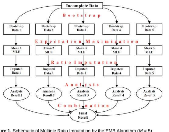
(8)Graphically outlined in Figure 1 is a schematic overview of multiple ratio imputation (M = 5). In summary, multiple ratio imputation replaces missing values by M simulated values, where M > 1. Conditional on observed data, the imputer constructs a posterior distribution of missing data, draws a random sample from this distribution, and creates several imputed datasets. Then, conduct the standard statistical analysis, separately using each of the M multiple-imputed datasets, and combine the results of the M statistical analyses in the above manner to calculate a point estimate just as in regular multiple imputation.
Figure 1. Schematic of Multiple Ratio Imputation by the EMB Algorithm (M = 5)
Monte Carlo Evidence
Using 45,000 simulated datasets with various characteristics, the Relative Root Mean Square Errors (RRMSE) of the estimators for the mean, the standard deviation, and the t-statistics in regression across different missing data handling techniques are compared. The data are a modified version of the simulated data used by King et al. (2001). The Monte Carlo experiments are based on 1,000 iterations, each of which is a random draw from the following multivariate normal distribution: Variables y1 and y2 are normally distributed with the mean vector (6, 10) and the standard deviation vector (1, 1), where the correlation between y1 and
y2 is set to 0.6 (Note that the value of 0.6 was chosen because this is approximately the correlation value among the variables in official economic statistics which is the target of the current study. Also, in other few runs, not reported, the parameter values were changed, and the conclusions were very similar). Each set of these 1,000 data is repeated for n = 50, n = 100, n = 200,
n = 500, and n = 1,000; thus, there are 5,000 datasets of five different data sizes. Our simulated data assume that the population model is equation (9).
1 2 , i i i Y
Y
where 1
2 0.6, i ~ 0, 0.64 . Y N Y
(9)Furthermore, following King et al. (2001), each of these 5,000 datasets is made incomplete using the three data generation processes of MCAR, MAR, and NI as in Table 5. Under the assumption of MCAR, the missingness of y1 randomly depends on the values of u (uniform random numbers). Under the assumption of MAR, the missingness of y1 depends on the values of y2 and u. Under the assumption of NI, the missingness of y1 depends on the observed and unobserved values of y1 itself and the values of u.
Table 5. Missingness Mechanisms and Missing Rates
MCAR Missingness of y1 is a function of u. 15%: y1 is missing if u > 0.85. 25%: y1 is missing if u > 0.75. 35%: y1 is missing if u > 0.65. MAR
Missingness of y1 is a function of y2 and u.
15%: y1 is missing if y2 > 10 and u > 0.7. 25%: y1 is missing if y2 > 10 and u > 0.5. 35%: y1 is missing if y2 > 10 and u > 0.3.
NI
Missingness of y1 is a function of y1, x, and u.
15%: y1 is missing if y1 > 6 and u > 0.7. 25%: y1 is missing if y1 > 6 and u > 0.5. 35%: y1 is missing if y1 > 6 and u > 0.3.
Variable y1 is the target incomplete variable for imputation, Variable y2 is completely observed in all of the situations to be used as the auxiliary variable, and Variable u in Table 5 is 1,000 sets of continuous uniform random numbers ranging from 0 to 1 for the missingness mechanism. The average missing rates are set to 15%, 25%, and 35%. These missing rates approximately cover the range from 10% to 40% missingness.
The performance can be captured by the Mean Square Error (MSE), defined as equation (10), where θ is the true quantity of interest and
ˆ is an estimator. The MSE measures the dispersion around the true value of the parameter, suggesting that an estimator with the smallest MSE is the best of a competing set of estimators (Gujarati, 2003, p. 901).
2ˆ ˆ
MSE E (10)
For the ease of interpretation, following Di Zio & Guarnera (2013), the Relative Root Mean Square Error (RRMSE) is used, which is defined as equation (11), where θ is the truth,
ˆ is an estimator, and T is the number of trials. For example, θ in the following analyses is the mean, the standard deviation, and thet-statistic based on complete data.
ˆ is the estimated quantity based on imputed data. T is 1,000.
2 1 ˆ 1 ˆ T t RRMSE T
(11)The complete results based on the 45,000 datasets are presented in Tables 6,
8, and 9. In the following analyses, the multiple ratio imputation model sets the number of multiple-imputed datasets (M) to 100, based on the recent findings in the multiple imputation literature (Graham et al., 2007; Bodner, 2008).
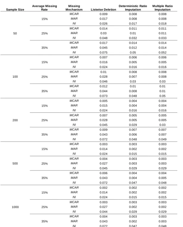
RRMSE Comparisons for the Mean
Presented in Table 6 are the RRMSE comparisons for the mean among listwise deletion, deterministic single ratio imputation, and multiple ratio imputation (M = 100), where the RRMSE is averaged over the 1,000 simulations. For multiple ratio imputation, the 100 mean values are combined using equation (7) in each of the 1,000 simulations.
The standard recommendation (de Waal et al., 2011, p.245) is that if the goal is to calculate a point estimate, the choice is deterministic single ratio imputation. Thus, the main purpose of this comparison is to show that the performance of multiple ratio imputation is as good as that of deterministic single ratio imputation, which is known to be a preferred method for the estimation of the mean. If multiple ratio imputation equally performs well compared to deterministic single ratio imputation, this means that multiple ratio imputation attains the highest performance in estimating the mean.
Table 6. RRMSE Comparisons for the Mean (45,000 Datasets)
Sample Size
Average Missing Rate
Missing
Mechanism Listwise Deletion
Deterministic Ratio Imputation Multiple Ratio Imputation 50 15% MCAR 0.009 0.008 0.008 MAR 0.017 0.008 0.008 NI 0.026 0.017 0.018 25% MCAR 0.014 0.011 0.011 MAR 0.03 0.01 0.011 NI 0.048 0.032 0.033 35% MCAR 0.017 0.014 0.014 MAR 0.045 0.012 0.014 NI 0.075 0.05 0.052 100 15% MCAR 0.007 0.006 0.006 MAR 0.016 0.005 0.005 NI 0.024 0.016 0.016 25% MCAR 0.01 0.008 0.008 MAR 0.028 0.007 0.008 NI 0.046 0.03 0.03 35% MCAR 0.012 0.01 0.01 MAR 0.044 0.008 0.01 NI 0.073 0.048 0.05 200 15% MCAR 0.005 0.004 0.004 MAR 0.015 0.004 0.004 NI 0.024 0.016 0.016 25% MCAR 0.007 0.005 0.005 MAR 0.028 0.005 0.005 NI 0.045 0.029 0.03 35% MCAR 0.009 0.007 0.007 MAR 0.043 0.006 0.007 NI 0.072 0.048 0.049 500 15% MCAR 0.003 0.003 0.003 MAR 0.014 0.002 0.002 NI 0.024 0.015 0.015 25% MCAR 0.004 0.003 0.003 MAR 0.027 0.003 0.003 NI 0.045 0.029 0.029 35% MCAR 0.006 0.004 0.004 MAR 0.043 0.004 0.005 NI 0.072 0.047 0.048 1000 15% MCAR 0.002 0.002 0.002 MAR 0.014 0.002 0.002 NI 0.024 0.015 0.015 25% MCAR 0.003 0.003 0.003 MAR 0.027 0.002 0.002 NI 0.044 0.029 0.029 35% MCAR 0.004 0.003 0.003 MAR 0.043 0.002 0.003 NI 0.072 0.047 0.048
In 42 of the 45 patterns, deterministic ratio imputation and multiple imputation both outperform listwise deletion with 3 ties. Even when the missing mechanism is MCAR, the results by imputation are almost always better than those of listwise deletion. Between the ratio imputation methods, deterministic ratio imputation slightly performs better than multiple ratio imputation in 14 out of the 45 patterns with 31 ties. However, the largest difference is only 0.002 in terms of the RRMSE. Thus, there are no significant differences between deterministic ratio imputation and multiple ratio imputation. Furthermore, this difference is expected to completely disappear as M approaches infinity. In general, under the situations where the model is correctly specified and the assumption of MAR is satisfied, both single imputation and multiple imputation (M = ∞) would be unbiased and agree on the point estimation (Donders et al., 2006). The results in Table 6 ensure this general relationship also applies to the relationship between single ratio imputation and multiple ratio imputation. Therefore, on average, multiple ratio imputation can be expected to give essentially the same answers as to the estimation of the mean, compared to deterministic ratio imputation.
Multiple ratio imputation can be more useful than deterministic single ratio imputation in the estimation of the mean, because multiple ratio imputation has more information in its output. Recall that there are three sources of variation in multiple imputation (van Buuren, 2012). One is the conventional measure of statistical variability (also known as within-imputation variance). Another is the additional variance due to missing values in the data (also known as between-imputation variance). The last one is simulation variance by the finite number of multiple-imputed data captured by
B
M/
M
in equation (8). Among these, the between-imputation variance is particularly important, because it reflects the uncertainty associated with missingness (Honaker et al., 2011).To demonstrate how multiple ratio imputation provides additional information on the between-imputation variance, presented in Table 7 is the mean of y1 when the missing data mechanism is MAR with the average missing rate of 35%, where the reported values are the average over the 1,000 simulations. In
Table 7, when the missing data mechanism is MAR, both of the imputation methods are almost equally accurate, in terms of estimating the mean. Additionally, multiple ratio imputation has more rows in Table 7 for BISD and CI (95%). BISD stands for the Between-Imputation Standard Deviation, and CI (95%) stands for the Confidence Interval associated with estimation error due to missingness at the 95% level. BISD is the square-root of the between-imputation
variance and measures the dispersion of the 100 mean values based on multiple ratio imputation (M = 100). In other words, BISD is the variation in the distribution of the estimated mean, which is usually called the standard error (Baraldi & Enders, 2010, p.16). Thus, based on BISD, the imputer can be approximately 95% confident that the true mean value of complete data is somewhere between 5.941 and 6.057, after taking the error due to missingness into account. Furthermore, the imputer can be approximately 95% confident that the imputed mean value (6.00) is meaningfully different from the listwise deletion estimate (5.74), which is outside the 95% confidence interval (5.94, 6.06). Single ratio imputation (both deterministic and stochastic) lacks this mechanism of assessing estimation uncertainty.
Table 7. Mean of y1 (MAR-35%)
Complete Data Listwise Deletion Deterministic Ratio Imputation Multiple Ratio Imputation Mean 6.000 5.741 6.000 5.999 BISD NA NA NA 0.029 CI (95%) NA NA NA 5.941, 6.057 n 500 325 500 500
Note. NA means Not-Applicable. Average over the 1,000 simulations. M = 100 for multiple ratio imputation
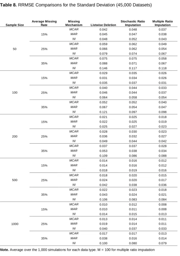
RRMSE Comparisons for the Standard Deviation
Presented in Table 8 are the RRMSE comparisons for the standard deviation among listwise deletion, stochastic single ratio imputation, and multiple ratio imputation (M = 100), where the RRMSE is averaged over the 1,000 simulations. For multiple ratio imputation, the 100 standard deviation values are combined using equation (7) in each of the 1,000 simulations.
The standard recommendation (de Waal et al., 2011) is that if the goal is to estimate the variation of data, the choice is stochastic single ratio imputation. Thus, the main purpose of this comparison is to show that the performance of multiple ratio imputation is as good as that of stochastic ratio imputation, which is known to be a preferred method to estimate the standard deviation. Note that, in other simulation runs, the EM algorithm was applied to the imputed data by the deterministic ratio imputation model, in order to compute the standard deviation. However, these results were not good and thus omitted here.
Table 8. RRMSE Comparisons for the Standard Deviation (45,000 Datasets)
Sample Size
Average Missing Rate
Missing
Mechanism Listwise Deletion
Stochastic Ratio Imputation Multiple Ratio Imputation 50 15% MCAR 0.042 0.048 0.037 MAR 0.045 0.047 0.038 NI 0.048 0.052 0.043 25% MCAR 0.059 0.062 0.049 MAR 0.066 0.062 0.054 NI 0.079 0.074 0.067 35% MCAR 0.075 0.075 0.058 MAR 0.088 0.071 0.067 NI 0.146 0.117 0.118 100 15% MCAR 0.029 0.035 0.026 MAR 0.031 0.034 0.026 NI 0.035 0.037 0.031 25% MCAR 0.040 0.044 0.033 MAR 0.046 0.044 0.037 NI 0.064 0.058 0.054 35% MCAR 0.052 0.052 0.040 MAR 0.067 0.054 0.047 NI 0.121 0.097 0.098 200 15% MCAR 0.021 0.025 0.018 MAR 0.022 0.025 0.019 NI 0.025 0.027 0.023 25% MCAR 0.028 0.030 0.023 MAR 0.036 0.032 0.027 NI 0.049 0.044 0.042 35% MCAR 0.037 0.037 0.028 MAR 0.053 0.038 0.034 NI 0.109 0.086 0.088 500 15% MCAR 0.014 0.016 0.012 MAR 0.014 0.016 0.012 NI 0.018 0.019 0.016 25% MCAR 0.018 0.020 0.015 MAR 0.024 0.020 0.017 NI 0.042 0.038 0.036 35% MCAR 0.022 0.023 0.018 MAR 0.043 0.024 0.021 NI 0.106 0.083 0.084 1000 15% MCAR 0.010 0.012 0.008 MAR 0.010 0.011 0.008 NI 0.014 0.015 0.013 25% MCAR 0.013 0.014 0.011 MAR 0.019 0.014 0.011 NI 0.040 0.037 0.033 35% MCAR 0.017 0.017 0.013 MAR 0.038 0.016 0.014 NI 0.100 0.080 0.079
In all of the 45 patterns, multiple ratio imputation always outperforms listwise deletion. Even when the missing mechanism is MCAR, the results by multiple ratio imputation are always better than those of listwise deletion. In contrast, stochastic ratio imputation outperforms listwise deletion in only 20 out of the 45 patterns. Especially, when the missing mechanism is MCAR, listwise deletion often outperforms stochastic ratio imputation in 11 out of the 15 patterns with 4 ties, although the difference is minimal. This implies that when missing data are suspected to be MCAR, there is a chance that using stochastic ratio imputation may make the situation worse than simply using listwise deletion. When the missing mechanism is MAR or NI, stochastic ratio imputation indeed outperforms listwise deletion in 20 out of the 30 patterns.
Between the ratio imputation methods, multiple ratio imputation often performs better than stochastic ratio imputation, 41 out of the 45 patterns. Therefore, this study contends that multiple ratio imputation is the preferred method for the estimation of the standard deviation. Table 8 implies that, regardless of missing mechanisms, multiple ratio imputation should be used for the purpose of estimating the standard deviation.
Just as in the case of estimating the mean, let us take the case of 35% missingness with the MAR condition as an example. Based on BISD, the imputer can be approximately 95% confident that the true standard deviation value of complete data is somewhere between 0.960 and 1.040, after taking the error due to missingness into account.
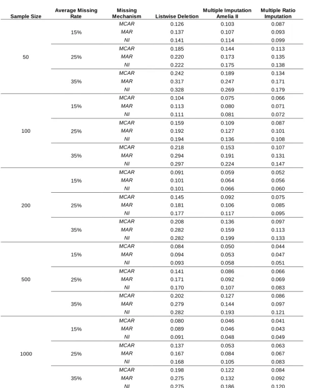
RRMSE Comparisons for the t-Statistics in Regression
The comparisons in this section are particularly important because even if the intercept should be zero and the slope should be estimated by the ratio between two variables, there are no other choices but to stick to regular multiple imputation for the computation of the t-statistics in regression. The regression model in Table 9 is y2 = a + b*y1. The quantity of interest is the t-statistic of b, i.e., tb = b ⁄ se(b) . The RRMSE reported here measures the average distance
between the true tb based on complete data and the estimated tb based on imputed
data. Table 9 presents the RRMSE comparisons for the t-statistics in regression among listwise deletion, regular multiple imputation (Amelia II), and multiple ratio imputation, where M = 100 for both regular multiple imputation and multiple ratio imputation, and the RRMSE is averaged over the 1,000 simulations. For regular multiple imputation and multiple ratio imputation, the 100 coefficient values are combined using equation (7), the 100 standard error values are
combined using equation (8), and the t-statistics are calculated using these two values in each of the 1,000 simulations.
Remember that the multiple ratio imputation model is equation (6). On the other hand, multiple imputation by Amelia II is equation (12), where the coefficients are random draws of the mean vectors and the variance-covariance matrices from the posterior distribution (Honaker & King, 2010).
1 0 1 2 i i i Y
Y
, where
1 2 1 0 1 1 2 2 cov , , var i i i Y Y Y Y Y
. (12)The standard recommendation (van Buuren, 2012; Hughes et al., 2014) is that if the goal is to obtain valid inferences with standard errors, the choice is multiple imputation which is a superior variance-estimation method. Thus, the main purpose of this comparison is to show that the performance of multiple ratio imputation is better than that of regular multiple imputation in terms of estimating the t-statistics. The comparison of the t-statistics in regression is appropriate, because it is the quantity of interest for many applied researchers in disputing whether an independent variable has some impact on a dependent variable. According to Cheema (2014), comparisons of t-statistics are fair because the complete sample and the imputed sample are identical in all respects including power, except for the fact that no values were missing in the complete sample while some values were missing in the imputed values. Therefore, the differences in the observed values of statistics are caused by the differences between imputed values and their true counterparts.
The comparison of multiple ratio imputation and Amelia II is appropriate, because the algorithm is the same EMB under the same platform of the R
statistical environment. In all of the 45 patterns, regular multiple imputation and multiple ratio imputation both outperform listwise deletion. Furthermore, multiple ratio imputation almost always outperforms regular multiple imputation 43 out of the 45 patterns under the condition where the true population model is equation (9). Thus, when the true model is a ratio model such as equation (9), multiple ratio imputation is more accurate and efficient than regular multiple imputation.
Therefore, multiple ratio imputation adds an important option for the tool kit of imputing and analyzing the mean, the standard deviation, and the t-statistics. If the true model is equation (9), multiple ratio imputation is at least as good as and in many cases better than the other traditional imputation methods for the three quantities of interest, regardless of the missingness mechanisms. However, it is
Table 9. RRMSE Comparisons for t-statistics (45,000 Datasets)
Sample Size
Average Missing Rate
Missing
Mechanism Listwise Deletion
Multiple Imputation Amelia II Multiple Ratio Imputation 50 15% MCAR 0.126 0.103 0.087 MAR 0.137 0.107 0.093 NI 0.141 0.114 0.099 25% MCAR 0.185 0.144 0.113 MAR 0.220 0.173 0.135 NI 0.222 0.175 0.138 35% MCAR 0.242 0.189 0.134 MAR 0.317 0.247 0.171 NI 0.328 0.269 0.179 100 15% MCAR 0.104 0.075 0.066 MAR 0.113 0.080 0.071 NI 0.111 0.081 0.072 25% MCAR 0.159 0.109 0.087 MAR 0.192 0.127 0.101 NI 0.194 0.136 0.108 35% MCAR 0.218 0.153 0.107 MAR 0.294 0.191 0.131 NI 0.297 0.224 0.147 200 15% MCAR 0.091 0.059 0.052 MAR 0.101 0.064 0.056 NI 0.101 0.066 0.060 25% MCAR 0.145 0.092 0.075 MAR 0.181 0.106 0.085 NI 0.177 0.117 0.095 35% MCAR 0.208 0.136 0.097 MAR 0.282 0.159 0.113 NI 0.282 0.199 0.133 500 15% MCAR 0.084 0.050 0.044 MAR 0.094 0.053 0.047 NI 0.093 0.058 0.051 25% MCAR 0.141 0.086 0.066 MAR 0.171 0.092 0.069 NI 0.170 0.107 0.083 35% MCAR 0.202 0.127 0.086 MAR 0.279 0.144 0.097 NI 0.282 0.193 0.121 1000 15% MCAR 0.080 0.046 0.041 MAR 0.089 0.046 0.043 NI 0.091 0.048 0.049 25% MCAR 0.137 0.053 0.063 MAR 0.167 0.084 0.067 NI 0.168 0.105 0.083 35% MCAR 0.198 0.122 0.084 MAR 0.275 0.132 0.092 NI 0.275 0.186 0.120
not claimed multiple ratio imputation is always superior to regular multiple imputation. If the true model is not a ratio model such as equation (9), the superiority shown in this section is not guaranteed.
Conclusion
A novel application of the EMB algorithm to ratio imputation was proposed, along with the mechanism and the usefulness of multiple ratio imputation. Monte Carlo evidence was presented, where the newly-developed R-function called
MrImputation (Takahashi, 2017) for multiple ratio imputation was applied to the 45,000 simulated data.
It was shown the fit of multiple ratio imputation was generally as good as or sometimes better than that of single ratio imputation and regular multiple imputation if the assumption holds. Specifically, for the purpose of estimating the mean, the performance of deterministic ratio imputation and multiple ratio imputation are essentially equally good, with multiple ratio imputation having additional information on estimation uncertainty. For the purpose of estimating the standard deviation, multiple ratio imputation outperforms stochastic ratio imputation. For the purpose of estimating the t-statistics in regression, multiple ratio imputation clearly outperforms regular multiple imputation when the population model is equation (9).
These findings are important because it is often recommended to use different ways of imputation depending on the type of statistical analyses, meaning that there are no one-size-fit-for-all imputation methods (Poston & Conde, 2014). Thus, multiple ratio imputation will be a valuable addition for treating missing data problems, so that multiple ratio imputation will expand the choice of missing data treatments.
This is only a starting point for multiple ratio imputation. There are three multiple imputation algorithms. The version of multiple ratio imputation introduced here used the Expectation-Maximization with Bootstrapping algorithm. However, multiple ratio imputation is a generic imputation model; thus, future research may apply the other two multiple imputation algorithms to expand the scope and the applicability of the method.
Acknowledments
The author wishes to thank Dr. Manabu Iwasaki (Seikei University), Dr. Michiko Watanabe (Keio University), Dr. Takayuki Abe (Keio University), Dr. Tetsuto
Himeno (Shiaga University), and Mr. Nobuyuki Sakashita (Statistical Research and Training Institute) for their valuable comments on earlier versions of this article. The author also wishes to thank the two anonymous reviewers for useful comments to revise this article. However, any remaining errors are the author's responsibility. Also, note that the views and opinions expressed in this article are the author's own, not necessarily those of the institution. The analyses in this article were conducted using R 3.1.0.
References
Allison, P. D. (2002). Missing Data. Thousand Oaks, CA: Sage Publications. Baraldi, A. N., & Enders, C. K. (2010). An introduction to modern missing data analyses. Journal of School Psychology, 48(1), 5-37. doi:
10.1016/j.jsp.2009.10.001
Bechtel, L., Gonzalez, Y., Nelson, M., & Gibson, R. (2011). Assessing several hot deck imputation methods using simulated data from several economic programs. Proceedings of the Section on Survey Research Methods, American Statistical Association, 5022-5036.
Bodner, T. E. (2008). What improves with increased missing data imputations? Structural Equation Modeling, 15(4), 651-675. doi:
10.1080/10705510802339072
Carpenter, J. R., & Kenward, M. G. (2013). Multiple Imputation and its Application. Chichester, West Sussex: John Wiley & Sons. doi:
10.1002/9781119942283
Cheema, J. R. (2014). Some general guidelines for choosing missing data handling methods in educational research. Journal of Modern Applied Statistical Methods, 13(2), 53-75.
Cochran, W. G. (1977). Sampling Techniques (3rd ed). New York, NY: John Wiley & Sons.
DeGroot, M H., & Schervish, M. J. (2002). Probability and Statistics (3rd ed). Boston, MA: Addison-Wesley.
de Waal, T., Pannekoek, J., & Scholtus, S. (2011). Handbook of Statistical Data Editing and Imputation. Hoboken, NJ: John Wiley & Sons. doi:
10.1002/9780470904848
Di Zio, M., & Guarnera, U. (2013). Contamination model for selective editing. Journal of Official Statistics, 29(4), 539-555. doi: 10.2478/jos-2013-0039
Do, C. B., & Batzoglou, S. (2008). What is the expectation maximization algorithm? Nature Biotechnology, 26(8), 897-899. doi: 10.1038/nbt1406
Donders, A. R. T., van der Heijden, G. J. M. G., Stijnen, T., & Moons, K. G. M. (2006). Review: A gentle introduction to imputation of missing values.
Journal of Clinical Epidemiology, 59(10), 1087-1091. doi:
10.1016/j.jclinepi.2006.01.014
Fox, J. (2015). Package ‘Norm’ [Computer software]. Retrieved from:
http://cran.r-project.org/web/packages/norm/norm.pdf
Graham, J. W., Olchowski, A. E., & Gilreath, T. D. (2007). How many imputations are really needed? Some practical clarifications of multiple
imputation theory. Prevention Science, 8(3), 206-213. doi: 10.1007/s11121-007-0070-9
Greene, W. A. (2003). Econometric Analysis (5th ed). Upper Saddle River, NJ: Prentice Hall.
Gujarati, D. N. (2003). Basic econometrics (4th ed). New York, NY: McGraw-Hill.
Honaker, J., & King, G. (2010). What to do about missing values in time series cross-section data. American Journal of Political Science, 54(2), 561-581. doi: 10.1111/j.1540-5907.2010.00447.x
Honaker, J., King, G., & Blackwell, M. (2011). Amelia II: a program for missing data. Journal of Statistical Software, 45(7), 1-47. doi:
10.18637/jss.v045.i07
Honaker, J., King, G., & Blackwell, M. (2015). Package ‘Amelia’ [Computer software]. Retrieved from:
http://cran.r-project.org/web/packages/Amelia/Amelia.pdf
Horowitz, J. L. (2001). The bootstrap. In J. J. Heckman & E. Leamer (Eds),
Handbook of Econometrics (pp. 3160-3228), Vol. 5. Amsterdam: Elsevier. doi:
10.1016/s1573-4412(01)05005-x
Hu, M., Salvucci, S., & Lee, R. (2001). A Study of Imputation Algorithms. Working Paper No. 2001–17. U.S. Department of Education. National Center for Education Statistics. Retrieved from: http://nces.ed.gov/pubs2001/200117.pdf
Hughes, R. A., Sterne, J. A. C., & Tilling, K. (2014). Comparison of imputation variance estimators. Statistical Methods in Medical Research, 25(6), 2541-2557. doi: 10.1177/0962280214526216
Iwasaki, M. (2002). Fukanzen Data no Toukei Kaiseki (Foundations of Incomplete Data Analysis). Tokyo: EconomistSha Publications, Inc.
King, G., Honaker, J., Joseph, A., & Scheve, K. (2001). Analyzing
incomplete political science data: an alternative algorithm for multiple imputation.
American Political Science Review, 95(1), 49-69.
Leite, W., & Beretvas, S. (2010). The performance of multiple imputation for Likert-type items with missing data. Journal of Modern Applied Statistical Methods, 9(1), 64-74.
Leon, S. J. (2006). Linear Algebra with Applications (7th ed). Upper Saddle River, NJ: Pearson/Prentice Hall.
Liang, H., Su, H., & Zou, G. (2008). Confidence intervals for a common mean with missing data with applications in AIDS study. Computational Statistics & Data Analysis, 53(2), 546-553. doi: 10.1016/j.csda.2008.09.021
Little, R. J. A., & Rubin, D. B. (2002). Statistical Analysis with Missing Data (2nd ed). Hoboken, NJ: John Wiley & Sons. doi: 10.1002/9781119013563
Long, J. S. (1997). Regression Models for Categorical and Limited Dependent Variables. Thousand Oaks, CA: Sage Publications.
Office for National Statistics. (2014). Change to imputation method used for the turnover question in monthly business surveys. Guidance and methodology: retail sales. Retrieved from: http://www.ons.gov.uk/ons/guide-method/method-quality/specific/economy/retail-sales/index.html
Poston, D., & Conde, E. (2014). Missing data and the statistical modeling of adolescent pregnancy. Journal of Modern Applied Statistical Methods, 13(2), 464-478.
Rubin, D. B. (1978). Multiple imputations in sample surveys: a
phenomenological Bayesian approach to nonresponse. Proceedings of the Survey Research Methods Section, American Statistical Association, 20-34.
Rubin, D. B. (1987). Multiple Imputation for Nonresponse in Surveys. New York, NY: John Wiley & Sons.
SAS Institute Inc. (2011). SAS/STAT 9.3 User’s Guide. Retrieved from:
http://support.sas.com/documentation/cdl/en/statug/63962/HTML/default/viewer. htm
Schafer, J. L. (1997). Analysis of Incomplete Multivariate Data. Boca Raton, FL: Chapman & Hall/CRC.
Seaman, S., Galati, J., Jackson, D., & Carlin, J. (2013). What is meant by “Missing at Random”? Statistical Science, 28(2), 257-268.
Shao, J. (2000). Cold deck and ratio imputation. Survey Methodology, 26(1), 79-85.
Shao, J., & Tu, D. (1995). The Jackknife and Bootstrap. New York, NY: Springer. doi: 10.1007/978-1-4612-0795-5
SPSS Inc. (2009). PASW Missing Values 18. Retrieved from:
http://www.unt.edu/rss/class/Jon/SPSS_SC/Manuals/v18/PASW Missing Values 18.pdf
Statistical Solutions. (2011). SOLAS Version 4.0 Imputation User Manual. Retrieved from:
http://www.solasmissingdata.com/wp-content/uploads/2011/05/Solas-4-Manual.pdf
Takahashi, M. (2017). Implementing multiple ratio imputation by the EMB algorithm in R. Journal of Modern Applied Statistical Methods, 16(1). doi:
10.22237/jmasm/1493598900
Takahashi, M., & Ito, T. (2013). Multiple imputation of missing values in economic surveys: comparison of competing algorithms. Proceedings of The 59th World Statistics Congress of the International Statistical Institute (ISI), 3240-3245.
Takahashi, M., Iwasaki, M., & Tsubaki, H. (2017). Imputing the mean of a heteroskedastic log-normal missing variable: A unified approach to ratio
imputation. Statistical Journal of the IAOS (forthcoming). doi: 10.3233/sji-160306
Thompson, K. J., & Washington, K. T. (2012). A response propensity based evaluation of the treatment of unit nonresponse for selected business surveys.
Federal Committee on Statistical Methodology 2012 Research Conference. Retrieved from:
https://fcsm.sites.usa.gov/files/2014/05/Thompson_2012FCSM_III-B.pdf van Buuren, S. (2012). Flexible Imputation of Missing Data. Boca Raton, FL: Chapman & Hall/CRC. doi: 10.1201/b11826
van Buuren, S., & Groothuis-Oudshoorn, K. (2011). mice: multivariate imputation by chained equations in R. Journal of Statistical Software, 45(3), 1-67. doi: 10.18637/jss.v045.i03
van Buuren, S., & Groothuis-Oudshoorn, K. (2015). Package ‘mice’ [Computer software]. Retrieved from: