User-assisted reverse modeling with evolutionary algorithms

User-assisted reverse modeling with evolutionary

algorithms

Pierre-Alain Fayolle

Alexander Pasko

Abstract—This paper presents a system for user-assisted reverse modeling: from digitized point-cloud to solid models ready to be used in a CAD modeling system. Our approach consists in the following steps: segmentation, fitting, and constructive model discovery. Each of these steps are based on evolutionary algorithms. The obtained objects can then be further edited or parameterized by users and fitted to adapt their shape to different point-clouds.

I. INTRODUCTION

Reverse engineering is the process of reconstruction from a scanned point-cloud of a geometric model ready to be used in a modeling system. In this work, we consider objects modeled in a constructive way by recursively applying geometric op-erations to primitives. Constructive Solid Geometry (CSG) is an example of such a constructive approach, where primitives correspond to quadrics and the operations include regularized Boolean operations and rigid transformations.

We are considering here evolutionary approaches to discov-ering a constructive model from a given scanned point-cloud. Our approach is based on the following steps: segmentation of the input point-cloud; fitting of primitives to each cluster; and discovery of a constructive model using these fitted primitives and geometric operations. The obtained constructive object can then be manipulated and edited by a user. A template model can also be extracted by a user with abstract parameters that can be fitted to adapt the shape to different point-clouds. We illustrate these steps with various experiments.

The main contributions of this work are:

• A general pipeline for constructive model recovery from point-clouds;

• Original evolutionary algorithms for constructive tree search using fitted primitives and set-theoretic opera-tions;

• Outline of the possible user interactive involvement at the different stages of the process.

II. RELATED WORK

A. Background on implicit surfaces and Function Representa-tion modeling

An implicit surface is a surface defined as the isovalue of a given function: {(x, y, z) :f(x, y, z) =c}, usuallyc= 0, see [1] and references therein. The Function Representation (see

[2]) considers solid as the point-set: {(x, y, z) : f(x, y, z)≥ 0}. Complex objects can be modeled using numerical tech-niques or procedurally by applying modeling operations to simpler primitives. The set operations (or boolean operations) can be implemented using min/max [3] or R-functions [2], [4]. For example set operations can be implemented with min/max as follow: S1∩S2:= min(fS1, fS2) (1) S1∪S2:= max(fS1, fS2) (2) ¯ S:=−fS (3) S1\S2:=S1∩S¯2 (4) where S, S1 and S2 are solids and fS, fS1 and fS2 their

corresponding functions.

This allows for representing a solid with a set-theoretic expression or equivalently by a function. In this work, solids are represented using this model.

B. Reverse engineering

Reverse engineering consists in transforming a digitized object into a computer model suitable for further processing. Surface reconstruction techniques in computer graphics consist generally in computing a triangle mesh approximating the shape, sometimes through the computation of an intermediate implicit surface (see e.g. [5] and references therein). Recent works are putting efforts on intelligent processing of acquired data: detection of symmetry and pattern, fitting of basic primitives, see for example the recent state of the art article [6] and the references it contains. In solid modeling, reverse engineering consists in retrieving accurate and consistent mod-els using standard surfaces from common CAD (Computer Aided Design) systems [7]. Some of the problems to be solved include: identifying sharp edges, treatment of blends, providing continuity and smoothness between the patches, and others [8]. C. Segmentation

A necessary step in most reverse engineering techniques is the segmentation of the input point-set, i.e. the clustering of the input data. There are various techniques available depending on the domain of application, see, for example, the section 1.1 of [9] for a more comprehensive survey of existing methods. Common techniques used in reverse engineering are also de-scribed in [10] (and references therein). After the segmentation step, patches need to be fitted to each cluster. This fitting step

can either be done separately from the segmentation step as, for example, in [11] or be done jointly with the segmentation as in [12]. The result of the segmentation and fitting can be improved by considering global relations between fitted primitives as in [13].

D. Constructive model discovery

Related to the problem of constructive model discovery is the problem of boundary representation to CSG conversion. Approaches to solve this problem are discussed in [14], [15]. These algorithms may require some additional halfspaces not available from the faces information or from the segmentation. An attempt to recover construction trees from point-cloud is discussed in [16]. The authors use strongly typed genetic programming. Parsimony is used to control the tree size. However, sizes of generated trees are still quite large. Fitting of primitives and construction tree extraction are performed together by genetic programming, making the approach un-suitable for complex objects. In [17], the authors use a genetic algorithm to evolve a linear tree with boolean operations in the nodes and given primitives in the leaves. However, for a given list of primitives, some objects can not be represented by a linear tree. In such case, the algorithm has to be iteratively applied reusing the best model obtained so far. We intend to improve the above approaches to the constructive model recovery and to propose an aoriginal solution suitable to wider clas of constuctive models.

III. OVERVIEW

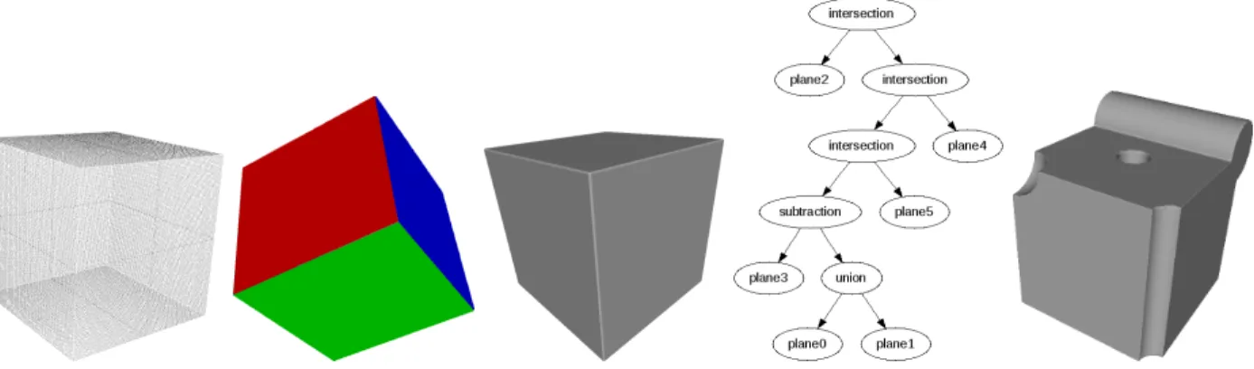
The input to our algorithm is a finite 3D point-cloud made of points sampled on the surface of a digitized object. We compute a constructive tree model for the object, made of primitives fitted to the point-cloud and connected by modeling operations. In the experiments described in section VIII, we use the following operations: union, intersection, complement and difference. Figure 1 illustrates the intermediate steps of our approach. The input point-cloud (left) is first segmented into clusters and primitives from a predefined set are fitted to each cluster (center-left). A constructive expression is then recovered that involves the fitted primitives and connect them by modeling operations (center-right). The expression can be imported in a constructive modeling system and further edited (right).

The main steps in our approach are:

• Point-cloud pre-processing: denoising, sub-sampling, normals computation;

• Segmentation and primitive fitting;

• Constructive tree discovery;

• Parameterization and fitting. IV. PRE-PROCESSING

The normal vector field is used in the fitting and construc-tive tree discovery steps. Some systems used for acquiring point-cloud data can sometimes retrieve this information. If the normal information is absent from the input point-cloud, we estimate it at a given point x of the input point-set by fitting the best plane using linear least square fitting over the

k-nearest neighbors ofx(in our experiments we usedk= 20). Orientation propagation is done following the algorithm given in [18]. For noisy point-sets, we are estimating normals using the approach described by Mitra et al in [19].

The algorithms described below can handle some noise in the input data without any further pre-processing. However, for objects severely corrupted by noise, it helps applying a denoising algorithm as a pre-processing step. The smoothing algorithms described by Jones et al. in [20] or Fleishman et al. in [21] give sufficiently good results. We can replace the connectivity information needed in these algorithms byk -nearest neighbor queries for cloud data. After the point-cloud has been smoothed, we re-estimate the normals using the updated points positions.

V. SEGMENTATION AND FITTING

A. RANSAC

The first step of our approach consists in the segmentation of the input point-set into clusters and fitting of primitives to each of these clusters. We also need to identify a primitive from a set of candidates, such as plane, sphere, cone or others, and fit its parameters to the points of each of the identified clusters. For this purpose, we can use the approach based on RANSAC [22] described in [12]. Given a finite point-set, the best fitted plane, sphere, cylinder, cone and torus to the point-set are computed using the RANSAC approach. Then the fitted primitive that best describes the data-set is selected and the corresponding points are removed from the point-set. In order to determine which of the fitted primitives best describes the data, the authors of [12] propose to count the number of points from the input point-setSthat are near the surface of the fitted primitive (see section 4.4 in [12]). These two steps are then repeated until the number of points left in the point-set is below some given threshold.

B. Evolutionary based segmentation

An alternative approach for fitting primitives from a list of candidates is described in [9]. For each type of primitive, its parameters maximizing an objective function are computed. The optimization is done in two steps: in the first step the objective function E1(p;f,P˜) in eq. 5 is maximized for the parameters p. In the second step, the optimal parameters are refined using the Levenberg-Marquardt algorithm [23], [24]. In [9], the first step optimization is performed by simulated-annealing. However, using a genetic algorithm gives similar results. The primitive best describing the data is then selected among all fitted primitives at this step and the corresponding points are removed from the point-set. These two steps are repeated until the number of points left in the point-set is below some given threshold.

1) Objective function: Given a primitive f and a point-cloud P˜, the parameters off are obtained by maximizing:

E1(p;f,P˜) =

N

X

i=1

exp(−di(p)2) +exp(−θi(p)2) (5)

where N is the number of points in the point-set P˜, P˜ is a uniform random subsampling of the original point-set P,

di(p) = f(xi;p)

d ,θi(p) =

ArcCos(|∇xf(xi;p)·n~i|)

Fig. 1. Overview of the approach: The input point-cloud (left) is segmented and primitives from a selected set are fitted to each cluster. Each fitted primitive is represented in its own color (center-left). A constructive model made of primitives and modeling operations is recovered: the center image shows the recovered solid and the center-right image the corresponding constructive expression as a tree with fitted primitives in the leaves and modeling operations in the nodes. Right: the edited object after addition of a cylinder and subtraction of a ball and cylinders.

Fig. 2. Points were sampled on a surface made of two ellipsoids. Left: segmentation and fitting using RANSAC. Right: segmentation and fitting with the approach described in section V-B.

This objective function is maximized for the vector p of unknown parameters of the current primitive f. With this objective function, the parameters p are penalized when the zero level-set of the corresponding primitive f(x;p) does not approximate well points in the point-cloud P or when

∇xf(x;p) does not align with the normal to the surface at

each point in P. The term exp(−θi(p)2) in (5) is used to

distinguish between two primitives with ”close” zero level-set. This method has the advantage over RANSAC of allowing for a larger set of possible primitives (such as ellipsoid or super-ellipsoid [25], for example). Consider, for example, Fig. 2. Points were artificially sampled on a surface obtained from two ellipsoids. The image on the left illustrates the segmentation result from the RANSAC based algorithm where each zone is identified as a part of a sphere. The right image shows the result of the method described in this section with the two identified ellipsoids.

C. Separating primitives

Primitives detected on the surface of an object are not always sufficient to describe the object when set operations are used. Sometimes it is necessary to introduce additional primitives that do not appear in the segmentation. These

Fig. 3. Additional primitives may be required to build a constructive representation from a boundary representation. The left object is a boundary representation of a simple two-dimensional solid, where each boundary patch has a different color. The right object contains an additional primitive, which is needed to build a constructive representation of the solid.

are called separating primitives or separators. The idea of introducing such primitives in order to describe an object by a CSG expression was introduced by Shapiro and Vossler in [14]. To illustrate the idea, consider the example in Fig. 3. The left part illustrates a boundary representation of a simple two-dimensional object, where each boundary patch has a different color. Building a constructive representation of this object, given the boundary patches, is not possible. An additional halfspace is required as illustrated in Fig. 3, right. The final CSG representation of the solid is given by:f =a∪b∩c∩d∩e. In order to compute separating primitives, we use the following method. First, we iterate through all the primitives identified during the segmentation step. If the current primitive is not a plane, we retrieve the set of points on or near this primitive. We compute the axis aligned bounding box corresponding to this point-set and add all the planes of the bounding box to the list of primitives obtained from the segmentation. If the plane to be added is already present in the list, we discard it. All identified separating primitives are added to the list of fitted primitives for the further steps of the recovery process.

VI. CONSTRUCTION TREE RECOVERY

We propose here some methods for recovering a model defined by a constructive tree (with geometric operations in internal nodes and primitives in leaves) from a point-cloud and a list of primitives. The list of primitives is obtained from the

previous steps. The goal is to automate the modeling process by providing ways to recover models that can be further edited, or parameterized and used as valid template models. Two evolutionary techniques are explored here: a genetic algorithm is first considered. Then a more generic approach based on genetic programming is described.

A. Genetic algorithm

Let us call P = {x1, . . . ,xn} the input point-cloud and

F = {f1, . . . , fm} the set of primitives fitted to the

seg-mented point-cloud. Given a finite set of geometric operations

{o1, . . . , ol}, we are searching for an ordering of the primitives

with operations acting on them such that the formula:

fi1oj1fi2. . . fim (6)

is a model for the solid corresponding to the point-cloud P. In the above expression, jk ∈ {1, . . . , l} (k ∈ {1, . . . , m})

and{i1, . . . , im} is a permutation of {1, . . . , m}. We assume

that all fitted primitives obtained from the previous steps are correctly oriented. Then we can restrict the list of operations to: union, intersection, difference, which are all binary operations. It simplifies the approach described below.

Pointsxi in the point-cloudP are on (or near) the surface

of the object, so we are searching for f = fi1oj1. . . fim

minimizing the least-square error: E2(f) = P_xi∈Pf(xi)2.

Following [17], a genetic algorithm is used for this minimiza-tion problem.

1) Genetic algorithm setting: An individual of the popu-lation represents a possible solution to the problem. In this case, it is an expression f. Each individual contains m pairs of integers (opk, Lk), 1 ≤ k ≤ m. In contrary to [17], we

represent these mpairs(opk, Lk)by an array of2mintegers.

Here,opk is an index in the set of possible operations. AndLk

corresponds to the position of the primitivekin the expression

f. The operation corresponding to opk is applied between the

primitivek(at the positionLk) and the preceding primitive (at

the positionLk−1) in the reconstructed expression. Because

there are only m −1 operations in an expression with m

primitives, we always ignore the operation paired with the primitive appearing at the first position.

Mutation With a given probability (using a uniform dis-tribution), a creature in the current population is mutated. A mutation point is obtained by sampling from an uniform distribution. There are two cases depending on whether the mutation point falls on an operation index (opk) or a primitive

position (Lk). If it falls on an operation index, then we can

simply select a new index at random. Otherwise, one of the primitives position Lk is randomly altered. The problem is

that we may then have two primitives at the same position: i.e. Li =Lj for somei6=j. The same type of problem can

happen after the crossover operation is applied. One way to resolve it is to sort the pairs opk, Lk with a stable sorting

algorithm. The position of the primitivekis then given by its position in the sorted array of pairs.

CrossoverPairs of creatures are subject to crossover with a given probability. A one-point crossover is used in the experiments. Similarly to the case of the mutation, a creature may contain two primitives at the same position after the

crossover operation is applied. We use the same technique as for the mutation operation to resolve this issue.

Selection Creatures to be included in the next population are selected using fitness proportionate selection (roulette wheel). We also always include the best creatures (two in the experiments) from the precedent population.

In [17], (6) is evaluated from left to right. It corresponds to a left-skewed tree structure with operations in the internal nodes and primitives in the leaves. However, not any given object can necessarily be represented by a left-skewed tree. The best creature is only an approximation of the object in such case. Since any object represented by a construction tree has an equivalent left-heavy tree, it is possible to iteratively re-apply the genetic algorithm re-using the best found creature as an additional primitive. In contrary we use a different approach in this work. Instead of evaluating (6) from left to right, we first evaluate the operations with higher precedence: intersection (∩) and difference (\).

B. Genetic programming

An alternative approach is to derive the expression (or the construction tree) by genetic programming [26]. A creature in the population corresponds to an expression with fitted primitives as leaves and geometric operations as internal nodes. A common approach is to use ”S-expressions” to represent the creatures and use a language that directly manipulates ”S-expression” such as Lisp to implement the genetic program-ming approach. Instead we are directly representing the tree in memory, and evaluate a given expression by tree traversal. It allows us to implement the approach with any programming language. The set of terminals (leaves) consists of all the fitted primitives (including separating primitives) obtained from the segmentation and fitting step. The set of functions (internal nodes) consists of geometric operations applied to the leaves and sub-trees. In our experiments, we used the traditional set-theoretic operations: union, intersection, difference and complement implemented with min/max (see section II-A).

For a given creature c and a finite point-set P, we need to assign a raw score to c. We use the following objective function E:

E3(c;P) =

N

X

i=1

(exp(−d2_i) +exp(−θ_i2))−λ size(c) (7) where:xi are the points from the input point-setP,N is the

number of points in the point-set, di = f(xi)

d , with f() is

the expression corresponding to the creature c and d a user

defined parameter, θi = ArcCos(−∇_αxf(xi)·n~i), with ∇xf the

gradient of the expression corresponding to the creaturec,n~i

the normal vector to the surface at the pointxi, and αa user

defined parameter,size()the function that counts the number of nodes (internal and leaves) in the tree corresponding to the creature c, andλa user defined parameter.

The goal is to maximizeE3(c, P)by genetic programming. Note the similarity of (7) with (5) used for segmentation in section V-B. One essential difference is the additional term

−λ size(c). This term is used in order to prevent trees to grow unnecessary large. For the coefficientλ, we used in our experiments log(N), where N is the size of the point-cloud.

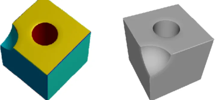
Fig. 4. Illustration of a parameterized template model: a model is built in a constructive way with abstract parameters that can be tuned to satisfy some modeling criteria.

Similarly to (5), this objective function smoothly penalizes expressions that do not pass on or near the points from the input point-set or have a gradient not aligned with the surface normal at each given point. The term exp(−θ2

i)) is used to

guarantee that the object is globally correctly oriented. It is also used to guarantee that locally the function behaves like a distance field (and therefore remove some potentially unwanted extra iso-surfaces).

We use standard implementation for the genetic operators: one-point crossover and one-point mutation. For the mutation, we either alter a given node in the tree or with a given probability (from a uniform distribution) replace a subtree at the given node by a new random creature. We use fitness proportionate selection.

VII. FITTING OF TEMPLATE MODELS

Once a constructive model has been recovered (even if only partially), it can be further edited (or completed if needed) and eventually can be parameterized to be re-used as a template model.

A. Template models

Given a constructive model, it is possible to identify various parameters (width of a box, radius of cylinder). The modifica-tion of these parameters can result in different shapes, which can also be tuned to fit some modeling criteria. Template model can exist in specialized libraries for each application domain (mechanical design, human prosthesis design, and others) and can be reused, or need to be created by a user. In the latter case, a modeling work needs to be done by a designer. An example of a parameterized template model, with different instances of its parameters, is illustrated in Fig. 4.

A template model can be written using its corresponding function as: f(x;p) where x corresponds to an evaluation point in the 3D space and p is a vector of parameters controlling the shape.

B. Fitting

Given a point-cloud S, the parameters p are optimized such that the isovalue {x : f(x;p) = 0} approximates the shape of the point-cloud. The parameters are obtained by optimizing an objective function E4 defined for a given template model f and a point-cloud P ={xi}. The simplest

choice for the objective function is to use the least square error: P

if

2_(x

i;p). This objective function should be minimized for

the vector of parameters p. An alternative choice is to use an objective function similar to what we used in (5) or in (7):E4(p;P) =Piexp(−

f2(xi;p)

σ2 ).E4 is maximized forp.

Fig. 5. A CAD object. Left: result of the segmentation. Right: recovered object by the genetic algorithm approach.

Either simulated annealing [27] or a genetic algorithm [28] with real encoded creature.

VIII. EXPERIMENTS

In this section, we illustrate with experiments the different steps of our approach. For the genetic algorithm and genetic programming technique, we are using large populations (at least100creatures). We are using a mutation rate high enough to avoid premature convergence to a local optimum (premature convergence to a uniform population). In these experiments, a mutation rate of 0.3 is used. In our experiments, we use a large number of iterations (at least 3000) and let the algorithm run until the end. In practice, one would implement some mechanism for trying to detect convergence (such as convergence to a uniform population or the value of the best creature(s) below/above some threshold).

A. Experiments with constructive tree recovery

a) Genetic algorithm: Figure 5 illustrates an example of point-cloud segmented (left), with primitives (plane, cylinder, sphere) fitted to each subset (in different colors), and the final object (right) obtained by the genetic algorithm approach described in section VI-A. The object’s surface is defined as: {(x, y, z) ∈ R3 : f(x, y, z) = 0} where f is the

expression recovered by the genetic algorithm. This surface is approximated by a triangle mesh using a meshing algorithm (the Marching Cubes algorithm [29]) and rendered with a typical mesh viewer.

One difficulty with the genetic algorithm approach is to extend it to work with the additional separating primitives computed in section V-C. A possible solution would be to include a boolean to each pair (opk, Lk), where the boolean

variable controls whether the primitivekshould be accounted for in the final expression or not. It makes the method more complicated to implement. The genetic programming based approach described in section VI-B seems a more natural approach.

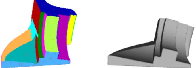
b) Genetic programming: Figure 6 illustrates the result of applying the genetic programming approach from section VI-B to a complex CAD shape (a fandisk). The input point-cloud is initially clustered in 23 segments with primitives iden-tified and fitted to each segment. The result of the segmentation is shown in Fig. 6, left, with each segment in a different color. The best creature found by genetic programming is

Fig. 6. Left: result of the segmentation and primitive fitting. Right: recovered object by genetic programming.

Fig. 9. A more complex CAD part recovered by our approach. Left: The input point-cloud. Right: The meshed recovered expression.

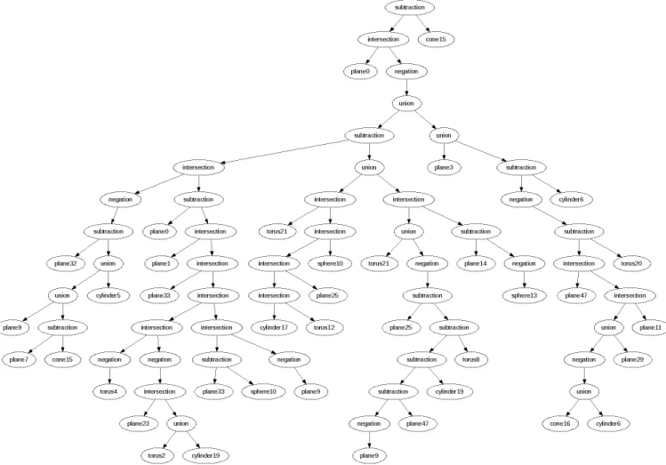
shown in Fig. 6, right. In this picture, the zero level-set of the best expression is approximated with a meshing algorithm as previously described. The resulting construction tree with geometric operations (Boolean) in the internal nodes and fitted primitives in the leaves is shown in Fig. 7.

The object shown in Fig. 6, right image, is the best creature found after 3000iterations of genetic programming. The raw fitness (7) of the best creature at each iteration is illustrated in the right graph, Fig. 8. Unless the input shape is relatively simple, the recovered object will be an approximation only. Approximation can occur in the segmentation and fitting stage. It can also occur in the genetic programming stage. The point-wise approximation error (using a log-scale) on the fandisk data-set is illustrated in Fig. 8 (left image). The point-wise error was obtained by evaluating the discovered expression f

at each point of the input point-cloud P. The middle picture in Fig. 6 shows the distribution of point-wise error.

Finally, Fig. 9 illustrates a more complex shape processed by the proposed approach. The input point-cloud consists in

280K points with normals.

B. User-assisted construction tree recovery

Given that we execute a fixed number of iterations in the genetic programming step, it is possible to get incomplete objects. The pot shown in Fig. 10 was incompletely recovered after 3000 iterations of genetic programming. A part of the handle was missing. The model was first edited by the user to remove the existing part. Then points from the input point-cloud that were not properly recovered were automatically identified by selecting points from the point-cloud with an error above some given threshold. The segmentation, fitting and genetic programming steps were then applied to this residual point-cloud in order to obtain the handle (see Fig. 10 second to right). Finally, the handle was attached to the rest of the object by using the union of the two recovered expressions (using (2)).

In the next experiment, we are trying to recover a freeform object from the point-cloud illustrated in Fig. 11, left. After the steps of segmentation, fitting and constructive tree recovery, we obtained the model illustrated in Fig. 11, middle. In this

example, approximation appears at different levels: fitting of primitives and constructive tree recovery. While the final result appears to be an interesting approximation and convey the overall shape of the object, one may want to improve the results. In order to obtain the result shown in Fig. 11, right image, the following additional steps were carried: First, the box approximating the horns was removed from the construc-tive model. Then, the set of points corresponding to the horns were isolated from the input point-cloud, and used to fit RBF splines [30]. Finally, we computed the union of the horns fitted by splines with the previous constructive model (from which the horns approximation was removed). The result is shown in Fig. 11, right image.

IX. CONCLUSION

We have presented in this paper our approach for discov-ering a constructive model from a given scanned point-cloud for an object. Our approach consists in: segmentation of the point-cloud, fitting primitives to it and discovery a constructive model using an evolutionary approach. Parameters can be extracted by a user from the model and fitted to adapt the shape to different point-clouds. Experiments illustrated some results obtained with our actual prototype. Perfect automation of the process is a difficult task and we plan to further incorporate user assistance in the different steps of the approach.

ACKNOWLEDGEMENT

The authors acknowledge the authors of [13] for providing the point-cloud used in Fig. 9. The point-clouds used in Fig. 6 and 11 is courtesy of AIM@SHAPE.

REFERENCES

[1] J. Bloomenthal, C. Bajaj, J. Blinn, M.-P. Cani-Gascuel, A. Rockwood, B. Wyvill, and G. Wyvill,Introduction to implicit surfaces. Morgan-Kaufmann, 1997.

[2] A. Pasko, V. Adzhiev, A. Sourin, and V. Savchenko, “Function repre-sentation in geometric modeling: concepts, implementation and appli-cations,”The Visual Computer, vol. 11, no. 8, pp. 429–446, 1995. [3] A. Ricci, “A constructive geometry for computer graphics,”The

Com-puter Journal, vol. 16, no. 2, pp. 157 – 160, 1973.

[4] V. Shapiro, “Theory of r-functions and applications: A primer,” Cornell University, Tech. Rep., November 1988.

[5] M. Kazhdan and H. Hoppe, “Screened poisson surface reconstruction,” ACM Transaction on Graphics, vol. 32, no. 3, pp. 29:1 – 29:13, 2013. [6] M. Berger, A. Tagliasacchi, L. Seversky, P. Alliez, J. Levine, A. Sharf, and C. Silva, “State of the art in surface reconstruction from point clouds,”Computer Graphics Forum, vol. 1, no. 1, pp. 1–xx, 2014. [7] T. Varady, R. Martin, and J. Cox, “Reverse engineering of geometric

models-an introduction,” Computer-Aided Design, vol. 29, no. 4, pp. 255–268, 1997.

[8] P. Benk´o, G. K´os, T. V´arady, L. Andor, and R. Martin, “Constrained fitting in reverse engineering,” Computer Aided Geometric Design, vol. 19, no. 3, pp. 173–205, 2002.

[9] P.-A. Fayolle and A. Pasko, “Segmentation of discrete point clouds using an extensible set of templates,” The Visual Computer, vol. 29, no. 5, pp. 449–465, 2013.

[10] T. V´arady, M. Facello, and Z. Ter´ek, “Automatic extraction of surface structures in digital shape reconstruction,” Computer-Aided Design, vol. 39, no. 5, pp. 379–388, 2007.

[11] M. Vanco and G. Brunnett, “Direct segmentation of algebraic models for reverse engineering,”Computing, vol. 72, no. 1, pp. 207–220, 2004.

Fig. 7. The construction tree for the fandisk model with geometric operations in the internal nodes and fitted primitives in the leaves.

Fig. 8. Left: Pointwise error (log scale) of the discovered object by genetic programming. Middle: Error distribution. Right: Raw fitness value of the best creature at each iteration of the genetic programming approach.

[12] R. Schnabel, R. Wahl, and R. Klein, “Efficient ransac for point-cloud shape detection,”Computer Graphics Forum, vol. 26, no. 2, pp. 214– 226, 2007.

[13] Y. Li, X. Wu, Y. Chrysathou, A. Sharf, D. Cohen-Or, and N. J. Mitra, “Globfit: Consistently fitting primitives by discovering global relations,” ACM Transactions on Graphics, vol. 30, no. 4, pp. 52:1–52:12, 2011. [14] V. Shapiro and D. Vossler, “Separation for boundary to CSG conver-sion,” ACM Transactions on Graphics (TOG), vol. 12, no. 1, p. 55, 1993.

[15] S. Buchele and R. Crawford, “Three-dimensional halfspace constructive solid geometry tree construction from implicit boundary representa-tions,”Computer-Aided Design, vol. 36, no. 11, pp. 1063–1073, 2004. [16] S. Silva, P.-A. Fayolle, J. Vincent, G. Pauron, C. Rosenberger, and C. Toinard, “Evolutionary computation approaches for shape modelling and fitting,” in Progress in Artificial Intelligence. Springer Berlin Heidelberg, 2005, pp. 144–155.

[17] P.-A. Fayolle, A. Pasko, E. Kartasheva, C. Rosenberger, and C. Toinard, “Automation of the volumetric models construction,” inHeterogeneous objects modelling and applications. Springer Berlin Heidelberg, 2008,

Fig. 10. User-assisted reverse modeling. Left: The original point-cloud. Middle: Intermediate object with the handle missing. Right: Final object with the handle fitted and attached to the object with the union operation.

Fig. 11. Left: The original point-cloud. Middle: Recovered constructive object. Right: Horns fitted by splines are used instead.

pp. 214–238.

[18] H. Hoppe, T. DeRose, T. Duchamp, J. McDonald, and W. Stuetzle, “Surface reconstruction from unorganized points,” inSIGGRAPH ’92: Proceedings of the 19th annual conference on Computer graphics and interactive techniques. New York, NY, USA: ACM, 1992, pp. 71–78. [19] N. J. Mitra, A. Nguyen, and L. Guibas, “Estimating surface normals in noisy point cloud data,” International Journal of Computational Geometry and Applications, vol. 14, no. 4-5, pp. 261–276, 2004. [20] T. Jones, F. Durand, and M. Desbrun, “Non-iterative, feature-preserving

mesh smoothing,”ACM Transactions on Graphics, vol. 22, no. 3, pp. 943–949, 2003.

[21] S. Fleishman, I. Drori, and D. Cohen-Or, “Bilateral mesh denoising,” ACM Transactions on Graphics, vol. 22, no. 3, pp. 950–953, 2003. [22] M. A. Fischler and R. C. Bolles, “Random sample consensus: a

paradigm for model fitting with applications to image analysis and automated cartography,”Commun. ACM, vol. 24, no. 6, pp. 381–395, 1981.

[23] K. Levenberg, “A method for the solution of certain non-linear problems in least squares,”The Quarterly of Applied Mathematics, pp. 164–168, 1944.

[24] D. Marquardt, “An algorithm for least-squares estimation of nonlinear parameters,”SIAM Journal on Applied Mathematics, vol. 11, pp. 431– 441, 1963.

[25] A. Barr, “Superquadrics and angle-preserving transformations,” IEEE Computer graphics and Applications, vol. 1, no. 1, pp. 11–23, 1981. [26] J. Koza,Genetic Programming. MIT Press, 1992.

[27] A. Corana, M. Marchesi, C. Martini, and S. Ridella, “Minimizing multi-modal functions of continuous variables with the “simulated annealing” algorithm,”ACM Trans. Math. Softw., vol. 13, no. 3, pp. 262–280, 1987.

[28] J. H. Holland, Adaptation in Natural and Artificial Systems. The University of Michigan Press, Ann Arbor, 1975.

[29] W. Lorensen and H. Cline, “Marching cubes: A high resolution 3d surface construction algorithm,” Computer Graphics, vol. 21, no. 4, 1987.

[30] Y. Ohtake, A. Belyaev, and H.-P. Seidel, “A multi-scale approach to 3d scattered data interpolation with compactly supported basis functions,” inShape Modeling International, 2003. IEEE, 2003, pp. 153–161.