UC Irvine Previously Published Works
Title
Channel Estimation and Performance Analysis of One-Bit Massive MIMO Systems
Permalink
https://escholarship.org/uc/item/6hn3t8fr
Journal
IEEE Transactions on Signal Processing, 65(15)
ISSN
1053-587X
Authors
Li, Yongzhi
Tao, Cheng
Seco-Granados, Gonzalo
et al.
Publication Date
2017-08-01
DOI
10.1109/tsp.2017.2706179
License
CC BY 4.0
Peer reviewed
eScholarship.org
Powered by the California Digital Library
Channel Estimation and Performance Analysis of
One-Bit Massive MIMO Systems
Yongzhi Li, Cheng Tao,
Member, IEEE,
Gonzalo Seco-Granados,
Senior Member, IEEE,
Amine Mezghani, A. Lee Swindlehurst,
Fellow, IEEE
and Liu Liu,
Member, IEEE,
Abstract—This paper considers channel estimation and system performance for the uplink of a single-cell massive multiple-input multiple-output (MIMO) system. Each receive antenna of the base station (BS) is assumed to be equipped with a pair of one-bit analog-to-digital converters (ADCs) to quantize the real and imaginary part of the received signal. We first propose an ap-proach for channel estimation that is applicable for both flat and frequency-selective fading, based on the Bussgang decomposition that reformulates the nonlinear quantizer as a linear function with identical first- and second-order statistics. The resulting channel estimator outperforms previously proposed approaches across all SNRs. We then derive closed-form expressions for the achievable rate in flat fading channels assuming low SNR and a large number of users for the maximal ratio and zero forcing receivers that takes channel estimation error due to both noise and one-bit quantization into account. The closed-form expressions in turn allow us to obtain insight into important system design issues such as optimal resource allocation, maximal sum spectral efficiency, overall energy efficiency, and number of antennas. Numerical results are presented to verify our analytical results and demonstrate the benefit of optimizing system performance accordingly.
Index Terms—massive MIMO, large-scale antenna systems, one-bit ADCs, channel estimation, power allocation
I. INTRODUCTION
Massive multiple-input multiple-output (MIMO) technology is considered to be a key component for 5G wireless com-munications systems, and has recently attracted considerable research interest. The main characteristic of massive MIMO is a base station (BS) array equipped with many (perhaps a hundred or more) antennas, which provides unprecedented
The research was supported in part by Beijing Nova Programme (Grant No. xx2016023), the NSFC project under grant No.61471027, the Research Fund of National Mobile Communications Research Laboratory, Southeast University (No.2014D05, No. 2017D01), and Beijing Natural Science Foun-dation project under grant No.4152043. A. Swindlehurst was supported by the National Science Foundation under Grant ECCS-1547155, and by the Technische Universit¨at M¨unchen Institute for Advanced Study, funded by the German Excellence Initiative and the European Union Seventh Framework Programme under grant agreement No. 291763, and by the European Union under the Marie Curie COFUND Program.
Y. Li, C. Tao, and L. Liu are with the Institute of Broadband Wireless Mobile Communications, Beijing Jiaotong University, Beijing, 100044, China (email: [email protected]; [email protected]; [email protected]).
G. Seco-Granados is with the Telecommunications and Systems Engineer-ing Department, Universitat Aut`onoma de Barcelona, Barcelona 08193, Spain (e-mail: [email protected]).
A. Mezghani and A. Swindlehurst are with the Center for Pervasive Communications and Computing, University of California, Irvine, CA 92697 USA (e-mail: [email protected]; [email protected]). A. Swindlehurst is also a Hans Fischer Senior Fellow of the Institute for Advanced Study at the Technical University of Munich.
Corresponding authors: [email protected], [email protected].
spatial degrees of freedom for simultaneously serving multiple user terminals on the same time-frequency channel. It has been shown that, with channel state information (CSI) available at the BS, relatively simple signal processing techniques such as maximum-ratio combining (MRC) or zero-forcing (ZF) can be employed to reduce the noise and interference at the terminals, and can lead to improvements not only in spectral efficiency, but in energy efficiency as well [1]–[5].
In most work on massive MIMO, perfect hardware imple-mentations with infinite resolution analog-to-digital converters (ADCs) are assumed. There has been limited prior work on the impact of non-ideal hardware on massive MIMO systems including [6]–[8], which studied imperfections such as phase-drifts and additive distortion, and showed that a massive number of antennas can mitigate these effects. In terms of hardware, perhaps the most important issue at the BS for massive MIMO is the power consumption of the ADCs, which grows exponentially with the number of quantization bits [9], and also grows with increased sampling rates due to wider bandwidths. For example, commercially available ADCs with resolutions of 12 to 16 bits consume on the order of several watts [10]. For massive MIMO configurations employing large antenna arrays and many ADCs, the cost and power consumption will be prohibitive, and alternative approaches are needed.
The use of low resolution (1-3 bits) ADCs is a potential solution to this problem [11]–[18]. In this paper, we focus on the case of simple one-bit ADCs, which consist of a simple comparator and consume negligible power (a few milliwatts). One-bit ADCs do not require automatic gain control and linear amplifiers, and hence the corresponding radio frequency (RF) chains can be implemented with very low cost and power consumption [17], [18]. It was shown in [11] that the capacity maximizing transmit signals for one-bit ADCs operating in single-input single-output (SISO) channels are discrete, unlike the infinite resolution case where a Gaussian codebook is optimal. In addition, [11] showed that MIMO capacity is not severely reduced by the coarse quantization at low signal-to-noise ratios (SNRs); in particular, the power penalty due to one-bit quantization is approximately equal
to only π/2 (1.96dB) in the low SNR region [12]. On the
other hand, at high SNRs one-bit quantization can produce a large capacity loss [19], but there is reason to believe that massive MIMO systems will operate at relatively low SNRs for improved energy efficiency, exploiting array gain to overcome the resulting distortion. This will be especially true as systems move to higher (e.g., millimeter wave) frequencies. In either
case, the availability of accurate BS-side CSI is indispensable for exploiting the full potential of a massive MIMO system, and an important open question is how to reliably estimate the channel and decode the data symbols under one-bit output quantization.
Several recent papers have investigated channel estimation in massive MIMO with one-bit ADCs [20]–[28]. A millimeter wave MIMO system with one-bit ADCs was considered in [24], which proposed a modified expectation-maximum (EM) channel estimator that exploits the sparsity of such channels. In [25] a near maximum likelihood (nML) channel estimator and detector were proposed, and the nML approach was shown to improve estimation accuracy and better support higher order constellations than the EM estimators using one-bit ADCs. However, the channel estimators and the computed rates obtained in [24], [25] rely on either the maximum-likelihood algorithm or on an iterative algorithm with high complexity, and their performance is difficult to theoretically quantify. More recently, [28] considered a low complexity channel estimator and the corresponding achievable rate for one-bit massive MIMO systems over frequency-selective channels, using a model in which the number of channel taps goes to infinity, and the quantization noise is essentially modeled as independent, identically distributed (i.i.d.) noise.
In this paper, we focus on channel estimation and uplink performance for massive MIMO systems with one-bit ADCs. In contrast to [28], we derive more general quantization noise models that are applied separately for data detection and channel estimation. One essential and unique aspect of our derivation is that the spatial correlation between the elements of the quantizer output is taken into account, calculated
using the arcsine law. Our goal is to illustrate the impact of
coarsely quantized ADCs, and to give an idea of the expected performance of massive MIMO systems with one-bit ADCs compared to conventional systems that assume infinite ADC resolution. Our specific contributions are summarized below.
• We focus on use of the Bussgang decomposition [29]
to reformulate the nonlinear quantizer operation as a statistically equivalent linear system. Contrary to previous work, we perform a separate Bussgang decomposition for the pilot and data phase as well as for each channel realization, an approach that more accurately captures the full effect of the quantization. We derive an algorithm that we refer to as the Bussgang Linear Minimum Mean
Squared Error (BLMMSE) channel estimator for both
flat and frequency-selective channel models. We calculate the high-SNR channel estimation error floor achieved by the proposed approach under flat fading, and show via simulation that BLMMSE outperforms previously proposed methods.
• We derive a lower bound for the flat-fading case on the
theoretical rate achievable in the uplink using MRC or ZF receivers based on the BLMMSE channel estimate, and we obtain a simple but tight closed-form approximation on the uplink rate assuming low SNR and a large number of users that accurately approximates our empirical obser-vations. Similar work in [30], [31] relied on an additive quantization noise model [32], [33] to approximate the
rate, but it assumed perfect rather than estimated CSI is available at the BS, which leads to an overly optimistic assessment.
• Using the closed-form expression for the achievable rate,
we study the power efficiency of massive MIMO with one-bit ADCs and show that similar efficiency is obtained as in conventional massive MIMO. In particular,
assum-ing M antennas, we show overall system performance
remains unchanged if 1) for a fixed level of CSI accuracy
(training data power independent of M), the transmit
power of each user terminal is reduced proportionally
to 1/M, and 2) power during both training and data
transmissions is reduced proportionally to1/√M.
• We propose an optimal resource allocation scheme to
maximize the sum spectral efficiency of a one-bit massive MIMO system under a total power constraint. Numerical results indicate that the optimal training length in one-bit systems is no longer always equal to the number of users and the proposed resource allocation scheme notably improves performance compared to the case without power allocation.
• We show that to achieve similar performance, a
one-bit massive MIMO system employing an MRC receiver will require approximately 2.2-2.3 times more antennas than a conventional system if the sum spectral efficiency for both systems is optimized by employing the optimal resource allocation scheme; for the ZF receiver, we show that to achieve the same goal, more and more antennas are needed as average transmit power increases.
A preliminary version of some of these results appeared in [34].
The rest of this paper is organized as follows. In the next section, we present the assumed system architecture and signal model. In Section III, we propose the BLMMSE channel estimator, and then based on the BLMMSE channel estimator, in Section IV we derive a simple closed-form expression for the lower bound on the achievable rate for MRC and ZF receivers in the low SNR region. Using the closed-form approximation, we then consider several system design issues related to resource allocation and the number of antennas in Section V. Simulation results are presented in Section VI and we conclude the paper in Section VII.
Notation: The following notation is used throughout the
paper. Bold uppercase (lowercase) letters denote matrices (vectors); (.)∗, (.)T, and (.)H denote complex conjugate,
transpose, and Hermitian transpose operations, respectively;
||.||represents the 2-norm of a vector; tr(.)represents the trace
of a matrix; diag{X} denotes a diagonal matrix containing
only the diagonal entries of X; ⊗ represents the Kronecker
product;[X]ij denotes the(i, j)th entry ofX;x∼ CN(a,B)
indicates that x is a complex Gaussian vector with mean a
and covariance matrixB; E{.}and Var{.}denote the expected value and variance of a random variable, respectively.
II. SYSTEMMODEL
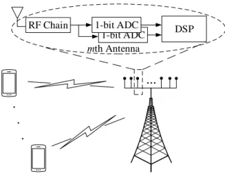
As depicted in Fig. 1, we consider a single-cell one-bit
mth Antenna
...
RF Chain DSP
K Users Base Station 1-bit ADC 1-bit ADC
Fig. 1: One-bit massive MIMO system architecture.
an M-antenna BS, where each antenna is equipped with two
one-bit ADCs and M K 1 is assumed. For the uplink,
we assume all K users simultaneously transmit independent
data symbols to the BS, so the received signal at the BS is
y=√ρdHs+n, (1)
wheren∼ CN(0,IM)is the M×1additive white Gaussian
noise vector, H is the M ×K channel matrix, and s is a
vector containing the signals transmitted by each user. We also
define the vectorized channelh= vec(H)and we assume that
h ∼ CN(0,Ch), where Ch is the covariance matrix of h.
We assume E{|sk|2}= 1, and we will define the scale factor
ρd to be the uplink SNR. Due to our assumption of one-bit
quantization below and hence the lack of any signal dynamic range, we must assume that some type of power control is implemented that prevents a strong user from overwhelming other weaker users. For this reason, in our model we assume
all users have the same level of large-scale fading/SNRρd.
The quantized signal obtained after the one-bit ADCs is represented as
r=Q(y) =Q(√ρdHs+n), (2)
where Q(.) represents the one-bit quantization operation,
which is applied separately to the real and imaginary part as Q(.) = √1
2(sign(<(.)) +jsign(=(.))). Thus, the output
set of the one-bit quantization is equivalent to the QPSK
constellation points R=√1
2{1 +j,1−j,−1 +j,−1−j}.
III. CHANNELESTIMATION FORONE-BITMIMO
In a standard implementation, the CSI is estimated at the BS and then used to detect the data symbols transmitted from
the Kusers. In the uplink transmission phase, we assume the
coherence interval is divided into two parts: one dedicated to training and the other to data transmission. During training,
allKusers simultaneously transmit their pilot sequences ofτ
symbols each to the BS, which yields
Yp=
√
ρpHΦT +Np, (3)
where Yp ∈ CM×τ is the received signal, ρp is the pilot
transmit power, andΦ∈Cτ×K is the pilot matrix transmitted
from theKusers. We assume all pilot sequences are
column-wise orthogonal, i.e., ΦTΦ∗ = τI
K, which implies τ ≥K.
We further assume that both SNRs ρd and ρp are known at
the BS via, for example, a low-rate control channel.
To match the matrix form of (3) to the vector form of (2), we vectorize the received signal as
vec(Yp) =yp= ¯Φh+np, (4)
whereΦ¯ = Φ⊗√ρpIMandnp =vec(Np). After one-bit
ADCs, the quantized signal can be expressed as
rp=Q(yp), (5)
where theith element ofrptakes values from the set R.
A. Bussgang-Based Channel Estimator
The authors in [21], [22], [24], [25] have investigated various methods for channel estimation in one-bit systems that rely on either the maximum-likelihood algorithm or on iterative algorithms with relatively high complexity. Further-more, the channel estimators obtained by these methods do not lend themselves to an analysis that provides insight on their performance.
To address these drawbacks, in this section we take a more fundamental approach and derive simple linear estimators whose performance can be analyzed in a straightforward way. These estimators are based on the so-called Bussgang decomposition [29], which finds a statistically equivalent (up to first and second moments) linear operator for any nonlinear function of a Gaussian signal. In particular, for the one-bit quantizer in (5), the Bussgang decomposition is written
rp=Q(yp) =Apyp+qp, (6)
whereApis the linear operator andqpthe statistically
equiv-alent quantizer noise. The matrix Ap is chosen to make qp
uncorrelated with yp [29], [35], or equivalently, to minimize
the power of the equivalent quantizer noise. This yields
Ap=CHyprpC
−1
yp, (7)
where Cyprp denotes the cross-correlation matrix between
the received signal yp and the quantized signal rp, and
Cyp denotes the auto-correlation matrix of yp. For one-bit
quantization and Gaussian inputs,Cyprp is given by [29][36,
Ch.10] Cyprp= r 2 πCypdiag Cyp −12 , r 2 πCypΣ −1 2 yp . (8)
whereΣyp = diag Cyp.
Using (4) and (6), we can expressrp as
rp=Q(yp) = ˜Φh+ ˜np, (9)
whereΦ˜ =ApΦ¯ ∈CM τ×M τ, n˜p=Apnp+qp∈CM τ×1.
For the sake of simplicity, we derive the subsequent formulas
for the case of Ch = IM K. We will show later in Section
VI.A that they are readily modified to include a generic Ch.
The matrix Apis given by substituting (8) into (7):
Ap=
r
2
πdiag Cyp
= r 2 πdiag ΦΦ H⊗ρ pIM+IM τ −1 2. (10)
We can see from (10) thatApdepends on the specific choice
of pilot sequencesΦ. In order to obtain a simple expression for
Ap, we will consider pilot sequences composed of submatrices
of the discrete Fourier transform (DFT) operator [37]. In
particular, we define Φ using K columns of the τ × τ
DFT matrix, in which case Φ has dimension τ×K, where
τ ≥K. The benefits of using DFT pilot sequences are: i) all
the elements of the matrix have the same magnitude, which simplifies peak transmit power constraints, and ii) the diagonal
terms of ΦΦH are always equal to K, which results in a
simple expression for Ap, as follows:
Ap= s 2 π 1 Kρp+ 1 IM τ ,αpIM τ. (11)
Based on this statistically equivalent linear model, we can formulate the LMMSE estimator [38], which we refer to as Bussgang LMMSE (BLMMSE) channel estimator:
ˆ
hBLM=ChrpC−1rprp=
˜
ΦH+ChqpC−1rprp, (12)
whereChrp is the cross-correlation matrix betweenhandrp,
Crp is the auto-correlation matrix ofrp.
The formula of (12) involves the auto-correlation function
of the quantized signal rp. It has been shown in [39] that for
one-bit ADCs, the arcsin law can be used to obtain
Crp =2 π arcsinΣ−12 yp < Cyp Σ−12 yp +jarcsinΣ−12 yp= Cyp Σ−12 yp . (13)
Moreover, using Ap as in (10) according to the Bussgang
theorem, the quantizer noise qp is not only uncorrelated
with the received signal yp, but also with the channel h
(see Appendix A). Therefore, we can simplify the BLMMSE channel estimator of (12) as
ˆ
hBLM= ˜ΦHC−1r
prp. (14)
Thus the covariance matrix of the BLMMSE channel esti-mate is given by
ChˆBLM = ˜ΦHC−1r
p
˜
Φ. (15)
A similar LMMSE channel estimator is proposed in [28]. However, our proposed channel estimator in (14) is more general since the correlation between each element of the quantizer noise is taken into account by using the arcsine law. In fact, (15) can be reduced to the estimator derived in
[28] if τ = K is assumed. When τ = K, it is easy to see
that Cyp = (Kρp+ 1)IM K, and hence according to (13),
Crp = IM K. Therefore, when τ = K we can obtain the
BLMMSE channel estimator of (14) as simply ˆ
hBLM= ˜ΦHrp. (16)
We emphasize that, when τ =K, there is no correlation
between the quantizer noise qp and the normalized MSE for
BLMMSE channel estimator is given by
MBLM= 1 M KE ˜ ΦHrp−h 2 2 = 1 M Ktr IM K−Φ˜HΦ˜ = 1− 2Kρp π(Kρp+ 1) , (17)
and for high SNRs lim ρp→∞M
BLM
= 1− 2
π =−4.40dB. (18)
The results in (17) and (18) are allied with the results in [28, Eq.(35)] by setting p[l] = 1/Land βkPk = ρp. In addition,
the result in (18) implies that there exists an error floor for the channel estimate as the training power increases to infinity.
B. Extension to Frequency Selective Fading with OFDM Although for simplicity we focus on the flat fading case in this paper, we show here how to extend our channel estimation method to the frequency selective case, assuming the transmit-ter employs OFDM signaling. In particular, consider an OFDM
system with Nc subcarriers, and denote the uplink OFDM
symbol transmitted from the kth user as xFD
k ∈ C Nc×1.
Before transmission, this vector is processed by a unitary IFFT
operation FH, and then a cyclic prefix (CP) of lengthN
cp is
added. Assume the CP length satisfies L−1 ≤ Ncp ≤ Nc,
whereLis the number of channel taps. After removing the CP,
theNc×1received time domain signal at themth BS-antenna
is given by yTDm = K X k=1 GTDmkFHxFDk +nTDm = K X k=1 ΦTDk gTDmk+nTDm = K X k=1 ΦTDk,LhTDmk+nTDm , (19) where the superscripts “TD” and “FD” refer to Time Domain
and Frequency Domain, respectively. The matrix GTDmk ∈
CNc×Nc is circulant and its first column is given by gTD
mk =
[(hTD
mk)
T,0, ...,0]T, where hTD
mk is an L×1 column vector
containing theL channel taps, andnTD
m ∼ CN(0,I)is
addi-tive white Gaussian noise. The matrixΦTD
k ∈C
Nc×Nc is also
circulant with first column given by φTD
k = F HxFD k . Φ TD k,L is a submatrix ofΦTD
k , corresponding to the firstL columns
of ΦTD
k . The second equation follows from the commutative
property of circulant convolution. The third equation is due to
the fact that there are only finiteLchannel taps.
After stacking the received time domain signalyTD
m for all M BS antennas, we have yTD= ¯ΦTDL hTD+nTD, (20) whereΦ¯TD L =I⊗ΦTDL withΦTDL = [ΦTD1,L,ΦTD2,L, ...,ΦTDK,L]∈ CNc×LK and hTD ∈
CM KL×1 contains all channel taps
between theM BS-antennas andKusers. After one-bit
quan-tization, the time domain quantized signal can be expressed as
and we see that, unlike a conventional system, OFDM cannot split the wideband channel into many parallel narrowband channel in a one-bit system.
Using the Bussgang decomposition, the non-linear quanti-zation operation can be reformulated as
rTD=AyTD+qTD
=AΦ¯TDL hTD+AnTD+qTD, (22)
where the matrixAis chosen to make the quantizer noiseqTD
uncorrelated withyTD. If the received time domain signalyTD
is Gaussian, we have A= r 2 πdiag CyTD −12 . (23)
Consequently, the BLMMSE channel estimator for the wide-band OFDM case can be expressed as
ˆ
hTD=ChTD( ¯ΦLTD)HAHC−1rTDr
TD, (24)
whereChTDis the covariance matrix ofhTD, and the
covari-ance matrix of rTD is obtained by using the arcsine law:
CrTD= 2 π arcsinΣ− 1 2 yTD< CyTD Σ− 1 2 yTD +jarcsinΣ− 1 2 yTD= CyTDΣ −1 2 yTD , (25) where ΣyTD = diag CyTD
. The covariance matrix of the
quantizer noise qTD can be obtained by
CqTD=CrTD−ACyTDAH. (26)
The above Bussgang-based channel estimators are more general than those derived in other work such as [28], since they take into account the fact that in general the covariance
matrix of the quantizer noise qTD cannot be expressed as a
diagonal matrix due to the arcsine law. This observation holds for any linear modulation scheme employed by the users, not just OFDM. While the derivations that follow will focus on the flat fading case, we can see from the above that they can be easily generalized to frequency-selective fading.
C. Low SNR Approximate BLMMSE Channel Estimate Co-variance
As we can see from (13) and (14), it is difficult to obtain a general closed-form expression for the MSE of the BLMMSE channel estimator due to the ‘arcsine’ operation. However, it is expected that massive MIMO systems will operate at relatively low SNRs due to the availability of a large array gain [2]. Therefore in this subsection, we focus on deriving a low-SNR approximation for the covariance matrix of the BLMMSE
channel estimator. According to (9), we can reformulate Crp
as the following linear function,
Crp= ˜ΦΦ˜ H+A pAHp +Cqp, (27) where Cqp=Crp−ApCypA H p = 2 π(arcsin(X) +jarcsin(Y))− 2 π(X+jY), (28)
and where we define
X=Σ−12 yp < Cyp Σ−12 yp (29) Y=Σ− 1 2 yp = Cyp Σ− 1 2 yp . (30)
We can see from (28) that the covariance matrix of the quantizer noise is in general not a diagonal matrix, which implies that there exists correlation between the quantization noise on each antenna. However, at low SNR or for large
numbers of users, Cyp is diagonally dominant and we can
use the following approximation for applying the arcsine law: 2 πarcsin(a) ∼ = 1, a= 1 2a/π, a <1. (31)
Since the non-diagonal elements ofXandYare much smaller
than 1 in the low SNR regime, we can approximate (28) as
Cqp∼= (1−2/π)IM τ. (32)
This implies that we can approximate the quantizer noise as
uncorrelated noise with a variance of 1−2/π at low SNR.
Substituting (32) and (27) into (15), we have
ChˆBLM ∼= ˜Φ HΦ˜Φ˜H+ (α2 p+ 1−2/π)IM τ −1 ˜ Φ = (α2pτ ρp+α2p+ 1−2/π)−1α2pτ ρpIM K,σ2IM K , (33)
where we have definedσ2= (α2pτ ρp+αp2+1−2/π)−1α2pτ ρp.
The equation on the second line holds due to the matrix
inversion identity(I+AB)−1A=A(I+BA)−1. The result
in (33) implies that in the low SNR regime, each element of the BLMMSE channel estimate is uncorrelated. In what follows, we will evaluate the uplink achievable rate by using the low SNR approximation in (33).
IV. ACHIEVABLERATEANALYSIS
IN THEONE-BITMIMO UPLINK
A. Data Transmission
In the data transmission stage, we assume the K users
simultaneously transmit their data symbols, represented as the
vector s, to the BS. After one-bit quantization, the signal at
the BS can be expressed as
rd=Q(yd) =Q(
√
ρdHs+nd)
=√ρdAdHs+Adnd+qd, (34)
where the same definitions as in the previous sections apply, but replacing the subscript ‘p’ with ‘d’, since the power
ρd during data transmission may be different than during
training. Again, according to the Bussgang decomposition and assuming a Gaussian input, we have
Ad= r 2 πdiag(Cyd) −1 2 = r 2 πdiag ρdHH H+I M −12. (35) Note that, in contrast to the model of [28], in which the quantizer noise can still be correlated with the desired signal since the same Bussgang decomposition is employed for different channel realizations, the Bussgang decomposition in (35) is employed for each individual channel realization. This
approach ensures that the quantizer noise is uncorrelated with the desired signal.
As can be seen in (35), the covariance matrix Cyd of the
quantizer input (and hence, the matrixHHH) must be known
at the BS in order to implement the Bussgang decomposition. In practice, however, we can use the same technique provided
in [40] to reconstruct the covariance matrix of Cyd using the
measurements of the quantizer output. In addition, relying on
channel hardening forK1 in massive MIMO systems and
for i.i.d. unit-variance channel coefficients, we can
approxi-mate the matrixAd as
Ad∼= r 2 π r 1 1 +Kρd IM =αdIM, (36)
without requiring perfect CSI. This approximate gain matrix is assumed without derivation in other previous work such as [28].
Next we assume the BS uses the BLMMSE channel estimate to compute a linear receiver to detect the data symbols
transmitted from the K users. The linear receiver attempts to
separate the quantized signal into K streams by multiplying
the signal by the matrix WT as follows:
ˆs=WTrd
=√ρdWTAd( ˆHs+Es) +WTAdnd+WTqd, (37)
where Hˆ = unvec(ˆhBLM) is the estimated channel matrix
(unvec is the inverse of the vec operator in Eq. (4)) and
E = H−Hˆ denotes the channel estimation error. The kth
element of ˆs is then used to decode the signal transmitted
from thekth user:
ˆ sk = √ ρdwTkAdhˆksk+ √ ρdwTk XK i6=kAd ˆ hisi +√ρdwkT XK i=1Adεisi+w T kAdnd+wTkqd, (38)
where wk, hˆk andεk are the kth columns ofW, Hˆ andE,
respectively.
The last four terms in (38) respectively correspond to user interference, channel estimation error, AWGN noise and quan-tizer noise. In our analysis, we will consider the performance of the common MRC and ZF receivers, defined by
WTMRC= ˆH H (39) WTZF= ˆ HHHˆ −1 ˆ HH, (40) respectively.
B. Uplink Achievable Rate Approximation at Low SNR Although prior work has obtained expressions for the mu-tual information or the achievable rate of one-bit systems using the joint probability distribution of the transmitted and received symbols [21], [23], [24], this approach does not result in easily computable or insightful expressions. To overcome this drawback, in this section we provide a simple closed-form expression for an approximation of the achievable rate for both MRC and ZF processing in the low SNR region. Using the
same reasoning as in Section III-C, the covariance matrix of
qd can be expressed as
Cqd=Crd−AdCydA
H
d, (41)
whereCrdis the covariance matrix ofrdand can be obtained
using the arcsine law in (13). Note that, again, the covariance matrix of (41) is in general not a diagonal matrix, which implies that there exists some correlations among the elements
of qd. For the special case where Cyd = ρdHH
H+I M is
diagonally dominant due to low SNR or for largeKwith i.i.d.
channels, then similar to the pilot phase, the approximation (32) can be used.
Furthermore, while the quantizer noiseqdis non-Gaussian,
we can obtain a lower bound on the achievable rate by making the worst-case assumption [41], [42] that in fact it is Gaussian with the same covariance matrix in (41). Using this approach and (38), the ergodic achievable rate of the one-bit MIMO uplink is lower bounded by (42) shown on the next page. In order to obtain a closed-form expression for the achievable rate, we rewrite the detected signal in (38) as a known mean gain (which only depends on the channel distribution instead of the instantaneous channel) times the desired symbol plus an uncorrelated effective noise, as follows:
ˆ
sk= E
√
ρdwkTAdhk sk+ ˜nd,k, (43)
where˜nd,k is the effective noise given by ˜ nd,k= √ ρdwkTAdhk−E √ ρdwTkAdhk sk +√ρdwkT K X i6=k Adhisi+wTkAdnd+wTkqd. (44)
Lemma 1: In a massive MIMO system with one-bit
quan-tization and Ad =αdIM, the uplink achievable rate for the
kth user at low SNR can be approximated by
Rk= log2 1 + ρdα2d E wT khk 2 ρdα2dVar wTkhk+UIk+AQNk ! , (45) where UIk=ρdα2d K X i6=k EnwkThi 2o (46) AQNk= α2d+ 1−2 π E n wTk 2o . (47)
Proof:See Appendix B.
The result in (45) is obtained by approximating the effective noise as Gaussian. In a massive MIMO system, the effective noise is a sum of a very large number of independent zero-mean terms, and thus we expect via the central limit theorem that the approximation will be asymptotically tight to the lower
bound of (42) inM. In Section V, it will be shown that the gap
between the achievable rate approximation given by (45) and the lower bound of the ergodic achievable rate given in (42) is small, which implies that our resulting closed-form expression is an excellent predictor of the system performance.
Based on Lemma 1, we derive in the theorems below closed-form expressions for the lower bound on the achievable rate
˜ Rk =E log2 1 + ρd w T kAdhˆk 2 ρdPKi6=k w T kAdhˆi 2 +ρdPKi=1 wkTAdεi 2 +wTkAd 2 +wT kCqdw ∗ k (42)
for the MRC and ZF receivers.
Theorem 1: For the MRC receiver with CSI estimated by
the BLMMSE channel estimator, the achievable rate of thekth
user in a one-bit massive MIMO uplink at low SNR can be approximated by RMRC,k= log2 1 + ρdα 2 dM σ 2 ρdα2dK+αd2+ (1−2/π) = log2 1 +ρdα2dM σ 2 . (48)
Proof: See Appendix C.
Theorem 2: For the ZF receiver with CSI estimated by the
BLMMSE channel estimator, the achievable rate of the kth
user in a one-bit massive MIMO uplink at low SNR can be approximated by RZF,k= log2 1 + ρdα 2 dσ2(M −K) ρdα2dKη+α 2 d+ (1−2/π) , (49) whereη= (1−σ2).
Proof: See Appendix D.
V. ONE-BITMASSIVEMIMO SYSTEMDESIGN
The simple approximation for the achievable rate derived in the previous section provides us with a tool for easily quantifying the impact of system design decisions. In this section, we study design issues surrounding the length of the training sequence, the power allocated for training and data transmission, and the number of BS antennas. Our perfor-mance metric will be the sum spectral efficiency, defined by
SA= T −τ T K X k=1 RA,k, (50)
whereTrepresents the length of the coherence interval, during
which the channel satisfies the block fading model and stays
constant. The notation A∈ {MRC,ZF} indicates that we will
perform the analysis for both the MRC and ZF receivers. A. Power Efficiency in One-Bit Massive MIMO
In this section, we study the power efficiency achieved by one-bit massive MIMO systems, where an increase in the number of antennas can be traded for reduced transmit power at the user terminals. We will consider two cases: i) the training
powerρp(and hence the channel estimation accuracy) is fixed,
but user transmit power decreases as1/M; and ii) the training
powerρpand data transmission powerρdare equal and scale
as 1/√M.
1) Case I: In the first case, we assume ρp is fixed and
independent of M, while ρd =Eu/Mc for a given c, where
Eu is fixed independent ofM. We will find the largest value
forcsuch that scaling down the users’ power by1/Mcresults
in no change in spectral efficiency as M → ∞. Substituting
ρd =Eu/Mc into (48) and (49) and assumingM increases
to infinity, we can readily see that choosingc= 1 will result
in the spectral efficiency converging to a fixed value. This implies that, when the channel estimation accuracy is fixed, the transmit power of each user can be reduced proportionally
by1/M for both the MRC and ZF receivers while maintaining
a given sum spectral efficiency. Moreover, the asymptotic performance for MRC and ZF is the same and is given by
lim M→∞SA|ρd=EMu = T−τ T Klog2 1 + 2 πσ 2E u . (51)
2) Case II: For the second case, we assume the training
and data transmission power are reduced at the same rate:
ρp=ρd =Eu/Mc, where againEu is fixed independent of
M. Substituting ρp =ρd = Eu/Mc into (48) and (49) and
assumingM increases to infinity, the value ofc= 1/2can be
seen to provide constant performance. Thus, we cannot reduce the user transmit power as aggressively as in the first case where the channel estimation accuracy is fixed. The asymptotic performance for MRC and ZF is again the same in this case, but with a different asymptotic value:
lim M→∞SA|ρd=ρp=√EMu = T−τ T Klog2 1 + 4 π2τ E 2 u . (52) Note that both of the spectral efficiency expressions in (51)
and (52) are equivalent to that of K SISO channels with
transmit power2σ2E
u/π and4τ Eu2/π2, respectively, without
interference. Thus, even though one-bit ADCs are deployed at the BS, the spectral efficiency increases proportionally to the
number of usersK.
B. Resource Allocation in One-Bit Massive MIMO System It has been proved in [41] that for conventional MIMO systems with infinite precision ADCs, the optimal training
length is always τ = K. However, due to the quantizer
noise, we will see that this result does not hold for one-bit massive MIMO systems. Considerable gains in spectral efficiency can be obtained by proper resource allocation. Thus in this subsection, we assume the users can vary the training power and the data transmission power and study the optimal resource allocation scheme that jointly selects the length of the training sequence, and the power allocated to training and data transmission with the goal of maximizing the sum spectral efficiency.
Let ρ be the average transmit power and P =ρT be the
total power budget for the users in one coherence interval,
which satisfies the constraint τ ρp+ (T −τ)ρd ≤ P. Then,
following the approach of [43], the optimization problem can be formulated as maximize ρp,ρd,τ SA subject to τ ρp+ (T −τ)ρd≤P K≤τ≤T (53)
ρp≥0, ρd≥0. (54)
For any power allocation in which the users do not employ the full energy budget, the users could increase their training power (and, thus, increase the channel estimation accuracy) without causing any inter-user interference in the data trans-mission phase, and hence in turn improve their rate. Therefore, we can replace the inequality constraint on the total energy budget with an equality constraint, i.e.,τ ρp+ (T−τ)ρd=P.
To facilitate the presentation, letγ∈(0,1)denote the fraction of the total energy budget that is devoted to pilot training, so
that γP =τ ρp and(1−γ)P = (T−τ)ρd. The optimization
problem in (53) is then equivalent to maximize
γ,τ SA|ρp=γPτ ,ρd=(1T−−γτ)P
subject to 0< γ <1, K≤τ≤T. (55)
Lemma 2: For both the MRC and ZF receivers in one-bit
massive MIMO, the optimal training lengthτ∗that maximizes
the sum spectral efficiency is not always equal to the number of users.
Proof: See Appendix E.
Although we cannot obtain a closed-form expression for
τ∗, we can numerically evaluate τ∗ using a simple search
algorithm since there are only a few parameters in problem (55). As we will show in the numerical results, unlike conven-tional MIMO systems, the optimal training duration depends on various system parameters such as the coherence interval
T and the total energy budget P.
C. How Many More Antennas are Needed for One-Bit Massive MIMO?
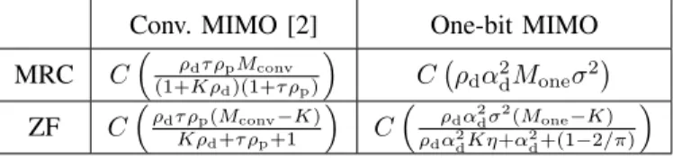
In this subsection, we compare the performance of one-bit and conventional massive MIMO with infinite resolution ADCs in terms of the number of antennas deployed at the BS. In particular, we wish to answer the question of how many more antennas a one-bit massive MIMO system would need to achieve the same spectral efficiency of a conventional massive MIMO implementation. For this analysis, we denote the number of antennas in the one-bit and conventional
mas-sive MIMO systems as Mone and Mconv, respectively, and
show the lower bound on the uplink achievable rate for both one-bit and conventional MIMO in Table I, where we define
C(x) =T−τ
T Klog2(1 +x).
For the special case of τ =K andρd=ρp, it was shown
in [28] that 2.5 times more antennas are needed in one-bit systems to ensure the same rate as the conventional system with MRC, and also for ZF at low SNR. This can be easily verified using our results as well. However, this result will
not hold in general for the optimal values of τ, ρd and ρp
resulting from the optimization in (55). In fact, we can pose a complementary optimization problem in which we attempt to
minimize the ratioκ=Mone/Mconvrequired for both systems
to achieve the same spectral efficiency, as follows: minimize γ,τ,κ κ subject to Sone A =S conv A , 0< γ <1, K≤τ≤T. (56)
TABLE I: Lower bound on individual achievable rates for conventional and one-bit MIMO systems
Conv. MIMO [2] One-bit MIMO
MRC C ρdτ ρpMconv (1+Kρd)(1+τ ρp) C ρdα2dMoneσ2 ZF Cρdτ ρp(Mconv−K) Kρd+τ ρp+1 C ρdα2dσ2(Mone−K) ρdα2dKη+α2d+(1−2/π) whereSconv
A is the maximum spectral efficiency achieved for
the conventional system by optimizing ρp andρd with τ =
K for fixed Mconv. Since the problem in (56) only has a
few parameters, we can use a simple search algorithm for the optimization.
Although no closed-form expression for the optimal κcan
be obtained, we will show in the simulations that less than 2.5 times more antennas are needed for the MRC receiver, and also for the ZF receiver at low SNR, if the training length
τ, training power ρp and data transmission power ρd are all
optimized.
VI. NUMERICALRESULTS
The simulation results presented here consider an uplink single-cell one-bit massive MIMO system with a coherence
interval ofT = 200 symbols. Unless otherwise indicated, we
assumeρp=ρd= SNR.
A. Channel Estimation Performance
In this subsection, we evaluate the performance of the BLMMSE channel estimator proposed in Section III-A com-pared with the LS channel estimator of [21] and the near maximum-likelihood channel estimator of [25]. Note that although the nML channel estimator proposed in [25] focused
on estimating the channel vector between the K users and
one receive antenna, we can define the nML estimator for the
entire channel for all M receive antennas and K users using
logic similar to [25] as follows: ˆ hnML= arg max ´ hR∈R2M K×1 kh´Rk2 ≤K 2M τ X i=1 logF√2 ¯ϕ(i)Rh´R , (57)
whereF(x)is the cumulative distribution function (CDF) of
the standard normal distribution, andϕ¯(i)R =√2rR,p(i)Φ¯(i)R .r(i)R,p
andΦ¯(i)R are respectively the ith element of rR,p and the ith
row ofΦ¯R: rR,p= [<(rp) =(rp)] T (58) ¯ ΦR= < Φ¯ −= Φ¯ = Φ¯ < Φ¯ . (59)
Figure 2 compares the MSE of the various channel
estima-tors as a function of SNR for a case with M = 16, K = 4
and τ = 20. Note that we also include the performance of
a similar channel estimator proposed in [28], in which the quantizer noise is modeled as uncorrelated additive noise with
a covariance matrix Cqp = (1−2/π)IM τ. We emphasize
again that in our work, the correlation between the elements of the quantization noise vector is taken into account using the
-20 -15 -10 -5 0 5 10 15 20 SNR (dB) -8 -6 -4 -2 0 2 4 6 8 Normalized MSE (dB) LS Proposed in [21]
near Maximum Likelihood in [25] BLMMSE
Additive Quantizer Noise in [28]
Fig. 2: MSE of channel estimators versus SNR with M =
16, K = 4 andτ = 20. Least Squares estimator is from [21]
and nML estimator is from [25].
arcsine law, and henceCqpis not in general a diagonal matrix.
We see that our proposed BLMMSE approach outperforms the other previously proposed approaches. We also see that at low SNR, BLMMSE and the method based on uncorrelated quantization noise achieves the same performance, which verifies the observation that the approximation of (32) is reasonable at low SNR. However, with the increase of SNR, a small performance gap can be seen between these two curves, indicating that not considering the correlation between the quantizer noise in one-bit systems may cause performance loss and the correlation should be taken into account.
A larger gap will result in cases where the quantizer noise is spatially correlated, since the analysis of [28] did not take this possibility into account. This will occur for example if the channel or the additive noise is itself spatially correlated.
For example, take the simple case depicted in Fig. 3 forM =
16, K = 1 and τ = 2, which shows the MSE performance
for a case with a spatially correlated channel where Ch is
non-diagonal. In this case, the BLMMSE channel estimator is given by
ˆ
hBLM=Ch(ApΦ¯)HC−1rprp, (60)
where, following the same step as in (7), the matrixAp is
Ap= r 2 πdiag ¯ ΦChΦ¯H+IM τ −12. (61)
For this example, we consider a typical urban channel model as described in [44], where the power angle spectrum of the channel is modeled by a Laplacian distribution with an
angle spread of 10◦. The covariance matrix Ch can then
be obtained according to [45, Eq. (2)]. We can see that the MSE performance gap grows to over 1 dB, indicating that the spatial correlation of the quantizer noise has an impact on performance and should be taken into account.
B. Validation of Achievable Rate Results
-20 -15 -10 -5 0 5 10 15 20 SNR (dB) -9 -8 -7 -6 -5 -4 -3 -2 -1 0 Normalized MSE (dB) BLMMSE
Additive Quantizer Noise in [28]
Spatially Correlated Channel
Fig. 3: MSE of channel estimators versus SNR with M =
16, K= 1 andτ= 2 over a spatially correlated channel.
-20 -18 -16 -14 -12 -10 -8 -6 -4 -2 0 SNR (dB) 0 5 10 15 20 25
Sum Spectral Efficiency (bits/s/Hz)
MRC, Monte-Carlo MRC, Analytical Results ZF, Monte-Carlo ZF, Analytical Results M= 32 M= 128 M= 64
Fig. 4: Sum spectral efficiency versus SNR with M =
{32,64,128} andK=τ = 8for MRC and ZF receivers.
Here we evaluate the validity of the lower bounds on the achievable rate for the MRC and ZF receivers derived in Theorems 1 and 2 compared with the ergodic rate given in (42). Fig. 4 shows the sum spectral efficiency versus
SNR with K = τ = 8 for different numbers of transmit
antennas M = {32,64,128}. The dashed lines represent
the sum spectral efficiencies obtained using the closed-form expressions in (48) and (49) for the MRC and ZF receivers, respectively, while the solid lines represent the ergodic sum spectral efficiencies obtained from (42). For both the MRC and ZF receiver, the gap between the approximation and the lower bound of the ergodic rate is small. For example, with
M = 128 and SNR = −10dB, the sum spectral efficiency
gap is 0.19 bits/s/Hz and 0.38 bits/s/Hz for the MRC and ZF receivers, respectively. This implies that the approximation on the achievable rate given in (45) is a good predictor of the performance of one-bit massive MIMO systems. Thus, in the following plots we will show only the approximation when evaluating performance.
50 100 150 200 250 300 350 400 450 500
Number of Receiver Antennas (M)
0 2 4 6 8 10 12
Sum Spectral Efficiency (bits/s/Hz)
MRC Receiver ZF Receiver Case I:;pis-xed,;d=Eu=M Case II:;p=;d=Eu= p M
Fig. 5: Sum spectral efficiency versus number of BS antennas
M for MRC and ZF receivers with ρp= 0dB, ρd =Eu/M
in Case I, andρp=ρd=Eu/ √ M in Case II. 100 101 0 5 10 15 20 25 30 35 Optimal Benchmark 100 101 Bit Energy 0 5 10 15 20 25 30 35
Sum Spectral Efficiency (bits/s/Hz)
Optimal Benchmark ZF Receiver M= 256 M= 128 MRC Receiver MRC Receiver ZF Receiver
Fig. 6: Bit energy versus sum spectral efficiency with and
without resource allocation for M ={128,256} andK= 8.
C. One-Bit Massive MIMO Power Efficiency
This example considers the power efficiency of using large antenna arrays in one-bit massive MIMO for the two cases considered in Section V-A. Fig. 5 shows the sum spectral
effi-ciency versus the number of receive antennas withK=τ = 8
for the MRC and ZF receivers for Cases I and II. In Case I,
we assume ρp = 10dB is fixed and ρd = Eu/M, while in
Case II we chooseρp=ρd=Eu/
√
M, whereEu= 0dB. As
predicted by the analysis, in Case I the sum spectral efficiency converges to the same constant value for both the MRC and
ZF receivers. In Case II where ρp = ρd = Eu/
√
M, the
sum spectral efficiency also converges to a constant value for both the MRC and ZF receivers, although the constant is only
reached for very largeM.
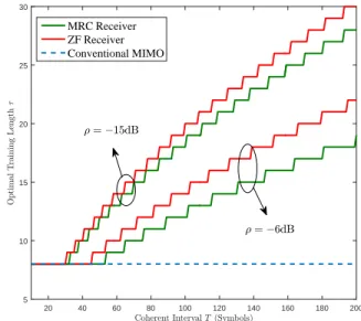
D. Resource Allocation
20 40 60 80 100 120 140 160 180 200
Coherent IntervalT(Symbols)
5 10 15 20 25 30 O p ti m al T ra in in g L en gt h = MRC Receiver ZF Receiver Conventional MIMO ;=!15dB ;=!6dB
Fig. 7: Optimal training length versus the coherence interval
withM = 128and average transmit powerρ={−15,−6}dB
for the MRC and ZF receivers.
We now investigate the benefit of our proposed optimal resource allocation scheme that adjusts the training length, training power, and data transmission power. In order to illus-trate the benefit achieved by our proposed allocation scheme, we define the bit energy as the total transmit power expended divided by the sum spectral efficiency, or energy consumed per transmitted bit:
ζA =
τ ρp+ (T−τ)ρd
SA
. (62)
Fig. 6 shows the sum spectral efficiency versus the bit
en-ergy with and without optimal power allocation for M =
{128,256} and for the MRC and ZF receivers. The
‘Bench-mark’ curves correspond to choosing τ = K and ρp = ρd,
while the ‘Optimal’ curves are obtained using the optimal resource allocation of (55). Different points on the curves correspond to different values of total available power. The benefit of an optimal power allocation is very evident in all cases. For example, to achieve a sum spectral efficiency of
15 bits/s/Hz with M = 128, the optimal resource allocation
can reduce the bit energy by a factor of 1.9 for both the MRC and ZF receivers compared to the benchmark case. The improvement in bit energy achieved by increasing the number of antennas is also apparent. For a sum spectral efficiency of
15bits/s/Hz and using the optimal resource allocation, we can
reduce the bit energy by a factor of about 2.2 for the MRC and ZF receivers, by doubling the number of antennas from 128 to 256.
Fig. 7 shows the optimal training duration versus the length
of the coherence interval for M = 128, K = 8 and average
transmit powerρ={−15,−6}dB for conventional and
one-bit massive MIMO systems. We can see that the optimal training length is always equal to the number of users for conventional massive MIMO systems, while it depends on the coherence interval and the total power budget for one-bit MIMO systems. This is because a larger proportion of the coherence interval devoted to training is required in
one-100 200 300 400 500 600 700 800 900 1000 Number of Antennas (M) 5 10 15 20 25 30 35 40 45 50
Sum Spectral Efficeincy (bits/s/Hz)
MRC, One-bit Massive MIMO ZF, One-bit Massive MIMO MRC, Conventional Massive MIMO ZF, Conventional Massive MIMO 100%
100%
73:68% 69:76%
Fig. 8: Comparison of the sum spectral efficiency versus num-ber of receive antennas for one-bit and conventional massive
MIMO systems with average transmit power ρ=−10dB.
bit systems to combat the quantization noise. In addition, we observe that the optimal training length for the MRC receiver is smaller than that for the ZF receiver, implying that the ZF receiver demands a higher quality channel estimate than MRC in order to reduce the interuser interference, and hence improve the sum spectral efficiency.
E. Number of Antennas for One-Bit and Conventional Massive MIMO
In this example we compare the sum spectral efficiencies between one-bit and conventional massive MIMO systems. Fig. 8 illustrates the sum spectral efficiency versus the number of receive antennas for the MRC and ZF receivers with an
average transmit power ρ = −10dB. Since we are more
interested in comparing the maximum sum spectral efficiencies of both one-bit and conventional systems, each curve is obtained by adjusting the training length, the training power and data transmission power to maximize the sum spectral efficiency, as in problem (55). The curves for ‘Conventional massive MIMO’ are obtained using the formulas in Table I. Compared with the conventional system, the rate loss of the one-bit system is not as severe as might be imagined. For
example, with M = 400, the one-bit system can still achieve
a sum spectral efficiency of 23.2 bits/s/Hz and 24.6 bits/s/Hz for the MRC and ZF receivers, respectively, which amounts
to 73.68% and 69.76% of the sum spectral efficiency of the
conventional system. This is a remarkably high value for such a coarsely quantized signal that only retains sign information about the received signals. The figure also verifies the increase in the number of antennas required for the one-bit system with MRC to achieve performance equivalent to a conventional massive MIMO system; the one-bit system requires about
480 antennas, or approximately 480/215 = 2.23 times more
antennas than for a conventional system to achieve a spectral efficiency of 25 bits/s/Hz.
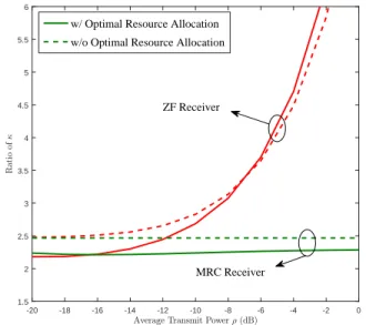
This relationship is further illustrated in Fig. 9 which shows
the ratio of κ = Mone/Mconv needed for the two types of
-20 -18 -16 -14 -12 -10 -8 -6 -4 -2 0
Average Transmit Power;(dB)
1.5 2 2.5 3 3.5 4 4.5 5 5.5 6 R at io of 5
w/ Optimal Resource Allocation w/o Optimal Resource Allocation
MRC Receiver ZF Receiver
Fig. 9: The ratio of κ versus the average transmit power ρ
withK= 8for the MRC and ZF receivers.
systems to achieve equivalent performance. The curves labeled
‘w/o Optimal Resource Allocation’ are obtained assumingτ=
K and ρp = ρd =ρ, while the curves labeled ‘w/ Optimal
Resource Allocation’ are obtained by solving problem (56). We can see that the ratio is constant at 2.5 for MRC and also at low SNR for ZF for the case without resource allocation, which verifies the conclusion in [28]. However, for the case with an optimal resource allocation, the ratio is around 2.2-2.3, which implies that fewer antennas are needed for the one-bit system if its performance is optimized. In addition, we see
that as the average transmit power ρ increases, the number
of antennas required for a one-bit system to have equivalent performance with the ZF receiver grows without bound, since the conventional ZF receiver is theoretically able to obtain a better and better channel estimate that allows it to ultimately eliminate all inter-user interference.
VII. CONCLUSIONS
This paper has investigated channel estimation and overall system performance for the single-cell, flat Rayleigh fading massive MIMO uplink when one-bit ADCs are employed at the BS. We used the Bussgang decomposition to derive a new channel estimator based on the LMMSE criteria, and showed that the resulting BLMMSE estimator provides the lowest MSE among various competing algorithms. However, even the BLMMSE estimator has a high-SNR error floor due to the one-bit quantization. We derived simple closed-form approximations for the massive MIMO uplink achievable rate for low SNR and a large number of users assuming MRC and ZF receivers that employ the BLMMSE channel estimate. We then used the approximation to study the sum spectral efficiency and energy efficiency of the one-bit massive MIMO uplink. Our results show that massive MIMO still yields similar gains in energy efficiency when one-bit quantizers are employed, and we developed an optimization problem that when solved yields significant gains in spectral efficiency by properly selecting the training length, training power and data
transmission power. We showed that for an MRC receiver with optimal resource allocation, approximately 2.2-2.3 times more antennas are required in a one-bit massive MIMO system to achieve the same spectral efficiency as a conventional system with full-precision ADCs. However, significantly more antennas are required in a one-bit system for the ZF receiver at high SNR. Finally, we presented a number of simulation results that validate our analysis and illustrate the potential performance of massive MIMO systems with one-bit ADCs.
APPENDIXA
For a givenyp, the covariance matrix between the quantizer
noiseqp and the channel vectorhcan be expressed as
EnqphH o =Eyp n EnqphH|yp oo . (63) Since the quantizer noiseqp=rp−Apypis fixed for a given
yp, we can remove qp from the inner expectation of (63) to
obtain Eyp n EnqphH|yp oo =Eyp n qpE n hH|yp oo . (64)
According to [38], the value of EnhH|yp
o
is the linear
MMSE estimate ofh, leading to
Eyp n EnqphH|yp oo =Eyp n qpyHpC −1 ypCyph o . (65)
Choosing Ap according to (7), the quantizer noise qp is
uncorrelated with yp, and hence we have
EnqphH o =Eyp n qpypHC−1ypCyph o =0, (66)
which implies that the quantizer noiseqpis uncorrelated with
the channel h.
APPENDIXB
We follow the approach of [46] and only exploit knowledge
of the average effective channel E√ρdwTkAdhk in the
detection. Then, according to [41], the lower bound of the achievable rate in (45) is obtained by treating the uncorrelated inter-user interference and the quantizer noise as independent Gaussian noise, which is a worst-case assumption when com-puting the mutual information [41]. Therefore the variance of the effective noise is
E{|n˜d,k|2}=Var wTkAdhk +ρd K X i6=k EnwTkAdhi 2o +EnwTkAd 2o +E wTkCqdwkT , (67) where the expectation operation is taken with respect to the channel realizations. By using the same result in (32) at low SNR, we can approximate the quantizer noise as
E wkTCqdwTk = 1− 2 π EnwTk 2o . (68)
Substituting Ad =αdIK and combining (67) and (68), we
arrive at Lemma 1.
APPENDIXC
From (45), we need to compute EwT
khk , Var wkThk
,
UIk andAQNk. Note that, although the channel vectorhk is
Gaussian, the BLMMSE channel estimatehˆk is not Gaussian
due to the quantizer noise. However, we can approximate hˆk
as Gaussian using Cram´er’s central limit theorem [47].
For the MRC receiverWT
MRC= ˆH H, we have wTkhk = ˆhHkhk= ˆ hk 2 + ˆhHk εk. (69) Therefore, EnhˆHkhk o =E ˆ hk 2 =M σ2. (70) The variance of wT khk is given by Var wkThk=E ˆ hHk hk 2 −M2σ4 =E ˆ hk 4 +E ˆ hHkεk 2 −M2σ4. (71)
Since hˆk is approximately Gaussian with variance of each
element M σ2, we obtain Var wTkhk=σ4M(M + 1) +σ2(1−σ2)M−M2σ4 =M σ2. (72) Fori6=kwe have UIk=ρdα2d K X i6=k E ˆ hHkhi 2 = (K−1)ρdα2dM σ 2. (73) Similarly, we obtain AQNk = (α2d+ 1−2/π)M σ2. (74)
Substituting (70), (72), (73) and (74) into (45), Theorem 1 is obtained.
APPENDIXD
For the ZF receiver WT
ZF= ˆ HHHˆ−1HˆH, we have WTZFH=WTZF( ˆH+E) =IK+WTZFE. (75) Therefore, wTZF,khk= 1 +wTZF,kεk. (76)
Similar to the derivation of the MRC receiver, we need to
compute EwT
khk , Var wTkhk
,UIk andAQNk.
For the ZF receiver, we have
E
wkThk = 1 +E
wTZF,kεk = 1. (77)
The variance of wTkhk is given by
Var wTkhk=E n wTZF,kεk 2o = (1−σ2)EnwTZF,k 2o = (1−σ2)E ( ˆ HHHˆ −1 k,k ) . (78)
SinceHˆ is approximately Gaussian,HˆHHˆ is aK×Kcentral
Wishart matrix withM degrees of freedom, Thus,
Var wTkhk
= (1−σ
2)
σ2(M −K). (79)
From (76), for i6=kwe have
UIk =ρdα2d K X i6=k E ˆ hHk εi 2 =ρdα2d K X i6=k (1−σ2)E ( ˆ HHHˆ −1 k,k ) = (K−1)ρdα2d (1−σ2) σ2(M−K). (80) Similarly, AQNk= α2 d+ 1−2/π σ2(M−K) . (81)
Substituting (77), (79), (80) and (81) into (45), Theorem 2 is obtained.
APPENDIXE
First we rewrite the sum spectral efficiency of (48) and (49)
for the MRC and ZF receivers as a function with respect toγ
andτ: SA(γ, τ) = T−τ T Klog2 1 + a1τ a2τ2+a3τ+a4 , (82) where we define a1= 4M P2(γ−γ2) a2=π2+ 2πP γ a3=π(KP(π−2)γ−KP(1−γ)(π+ 2P γ)−(π+ 2P γ)T) a4=π(K2P2(π−2)(−1 +γ)γ−KP(π−2)γT) for A=MRC, and a1= 4(M −K)P2(γ−γ2) a2=π2+ 2πP γ a3=−KP(2π(γ+P(γ−γ2)) + 4P(γ−γ2) +π2(2γ−1)) −(π2+ 2πP γ)T a4=π(K2P2(π−2)(−1 +γ)γ−KP(π−2)γT) for A=ZF.
Then we denote {γ∗, τ∗} to be the solution of (55), such
that γ∗P = τ∗ρ∗p is the optimal power for training, and
(1 −γ∗)P = (T −τ∗)ρ∗d is the optimal amount for data
transmission. Next we choose ¯τ = K,ρ¯p = γ∗P/τ¯ and
¯
ρd = (1−γ∗)P/(T −τ¯). Clearly, the function in (82) is
not a monotonic function with respect to τ with a given γ∗.
That is to say, it is difficult to compare the values ofS(γ∗, τ∗) andS(γ∗,τ¯). Therefore, we conclude that the optimal training length is not always equal to the number of users for one-bit systems.
REFERENCES
[1] T. Marzetta, “Noncooperative cellular wireless with unlimited numbers of base station antennas,”IEEE Transactions on Wireless Communica-tions, vol. 9, no. 11, pp. 3590–3600, November 2010.
[2] H. Q. Ngo, E. Larsson, and T. Marzetta, “Energy and spectral efficiency of very large multiuser MIMO systems,”IEEE Transactions on Com-munications, vol. 61, no. 4, pp. 1436–1449, April 2013.
[3] E. Larsson, O. Edfors, F. Tufvesson, and T. Marzetta, “Massive MIMO for next generation wireless systems,”IEEE Communications Magazine, vol. 52, no. 2, pp. 186–195, February 2014.
[4] F. Rusek, D. Persson, B. K. Lau, E. Larsson, T. Marzetta, O. Edfors, and F. Tufvesson, “Scaling up MIMO: Opportunities and challenges with very large arrays,”IEEE Signal Processing Magazine, vol. 30, no. 1, pp. 40–60, Jan 2013.
[5] L. Lu, G. Y. Li, A. L. Swindlehurst, A. Ashikhmin, and R. Zhang, “An overview of massive MIMO: Benefits and challenges,”IEEE Journal of Selected Topics in Signal Processing, vol. 8, no. 5, pp. 742–758, 2014. [6] E. Bj¨ornson, J. Hoydis, M. Kountouris, and M. Debbah, “Massive MIMO systems with non-ideal hardware: Energy efficiency, estimation, and capacity limits,”IEEE Transactions on Information Theory, vol. 60, no. 11, pp. 7112–7139, Nov 2014.
[7] E. Bj¨ornson, M. Matthaiou, and M. Debbah, “Massive MIMO with non-ideal arbitrary arrays: Hardware scaling laws and circuit-aware design,”
IEEE Transactions on Wireless Communications, vol. 14, no. 8, pp. 4353–4368, Aug 2015.
[8] X. Zhang, M. Matthaiou, M. Coldrey, and E. Bj¨ornson, “Impact of residual transmit RF impairments on training-based MIMO systems,”
IEEE Transactions on Communications, vol. 63, no. 8, pp. 2899–2911, Aug 2015.
[9] R. Walden, “Analog-to-digital converter survey and analysis,” IEEE Journal on Selected Areas in Communications, vol. 17, no. 4, pp. 539– 550, Apr 1999.
[10] “Texas instruments ADC products.” [Online]. Available: http://www.ti. com/lsds/ti/data-converters/analog-to-digital-converter-products.page [11] A. Mezghani and J. Nossek, “Analysis of Rayleigh-fading channels
with 1-bit quantized output,” in IEEE International Symposium on Information Theory (ISIT), July 2008, pp. 260–264.
[12] J. A. Nossek and M. T. Ivrlaˇc, “Capacity and coding for quantized MIMO systems,” in Proceedings of the international conference on Wireless communications and mobile computing. ACM, 2006, pp. 1387–1392.
[13] A. Mezghani, M.-S. Khoufi, and J. Nossek, “A modified MMSE receiver for quantized MIMO systems,” inProc. ITG/IEEE Workshop on Smart Antennas (WSA), Feb 2007.
[14] A. Mezghani, M. Rouatbi, and J. Nossek, “An iterative receiver for quantized MIMO systems,” in IEEE Mediterranean Electrotechnical Conference (MELECON), March 2012, pp. 1049–1052.
[15] A. Mezghani and J. Nossek, “Efficient reconstruction of sparse vectors from quantized observations,” inInternational ITG Workshop on Smart Antennas (WSA), March 2012, pp. 193–200.
[16] J. Singh, O. Dabeer, and U. Madhow, “On the limits of communication with low-precision analog-to-digital conversion at the receiver,” IEEE Transactions on Communications, vol. 57, no. 12, pp. 3629–3639, December 2009.
[17] J. Mo and R. W. Heath Jr., “Capacity analysis of one-bit quantized MIMO systems with transmitter channel state information,”IEEE Trans-actions on Signal Processing, vol. 63, no. 20, pp. 5498–5512, Oct 2015. [18] J. Singh, S. Ponnuru, and U. Madhow, “Multi-gigabit communication: The ADC bottleneck,” in IEEE International Conference on Ultra-Wideband (ICUWB), Sept 2009, pp. 22–27.
[19] J. Mo and R. W. Heath Jr., “High SNR capacity of millimeter wave MIMO systems with one-bit quantization,” inInformation Theory and Applications Workshop (ITA), 2014, Feb 2014.
[20] N. Liang and W. Zhang, “Mixed-ADC massive MIMO,”IEEE Journal on Selected Areas in Communications, vol. 34, no. 4, pp. 983–997, April 2016.
[21] C. Risi, D. Persson, and E. G. Larsson, “Massive MIMO with 1-bit ADC.” [Online]. Available: http://arxiv.org/abs/1404.7736
[22] S. Jacobsson, G. Durisi, M. Coldrey, U. Gustavsson, and C. Studer, “One-bit massive MIMO: Channel estimation and high-order modula-tions,” inIEEE International Conference on Communication Workshop (ICCW), 2015, June 2015, pp. 1304–1309.
[23] ——, “Throughput analysis of massive MIMO uplink with low-resolution ADCs.” [Online]. Available: https://arxiv.org/abs/1602.01139 [24] J. Mo, P. Schniter, N. Gonz´alez-Prelcic, and R. W. Heath Jr., “Channel estimation in millimeter wave MIMO systems with one-bit quantization,” in48th Asilomar Conference on Signals, Systems and Computers, 2014, Nov 2014, pp. 957–961.
[25] J. Choi, J. Mo, and R. W. Heath Jr., “Near maximum-likelihood detector and channel estimator for uplink multiuser massive MIMO systems with
one-bit ADCs,”IEEE Transactions on Communications, vol. 64, no. 5, pp. 2005–2018, May 2016.
[26] C. Moll´en, J. Choi, E. G. Larsson, and R. W. Heath Jr., “Performance of linear receivers for wideband massive MIMO with one-bit ADCs,” in
International ITG Workshop on Smart Antennas (WSA), March 2016. [27] ——, “One-bit ADCs in wideband massive MIMO systems with OFDM
transmission,” inIEEE International Conference on Acoustics, Speech and Signal Processing (ICASSP), March 2016, pp. 3386–3390. [28] ——, “Uplink performance of wideband massive MIMO with one-bit
ADCs,”IEEE Transactions on Wireless Communications, vol. 16, no. 1, pp. 87–100, 2017.
[29] J. J. Bussgang, “Crosscorrelation functions of amplitude-distorted Gaus-sian signals,” MIT Research Lab. Electronics, Tech. Rep. 216, 1952. [30] L. Fan, S. Jin, C.-K. Wen, and H. Zhang, “Uplink achievable rate for
massive MIMO systems with low-resolution ADC,”IEEE Communica-tions Letters, vol. 19, no. 12, pp. 2186–2189, Dec 2015.
[31] J. Zhang, L. Dai, S. Sun, and Z. Wang, “On the spectral efficiency of massive MIMO systems with low-resolution ADCs,”IEEE Communi-cations Letters, vol. 20, no. 5, pp. 842–845, 2016.
[32] O. Orhan, E. Erkip, and S. Rangan, “Low power analog-to-digital con-version in millimeter wave systems: Impact of resolution and bandwidth on performance,” in Information Theory and Applications Workshop (ITA), Feb 2015, pp. 191–198.
[33] Q. Bai, A. Mezghani, and J. A. Nossek, “On the optimization of ADC resolution in multi-antenna systems,” inProceedings of the Tenth International Symposium on Wireless Communication Systems (ISWCS),, Aug 2013.
[34] Y. Li, C. Tao, L. Liu, G. Seco-Granados, and A. L. Swindlehurst, “Chan-nel estimation and uplink achievable rates in one-bit massive MIMO systems,” inIEEE Sensor Array and Multichannel Signal Processing Workshop (SAM), July 2016.
[35] A. Mezghani and J. A. Nossek, “Capacity lower bound of MIMO channels with output quantization and correlated noise,” inIEEE Inter-national Symposium on Information Theory Proceedings (ISIT), 2012. [36] A. Papoulis and S. U. Pillai, Probability, Random Variables, and
Stochastic Processes. Tata McGraw-Hill Education, 2002.
[37] M. Biguesh and A. B. Gershman, “Downlink channel estimation in cel-lular systems with antenna arrays at base stations using channel probing with feedback,”EURASIP Journal on Applied Signal Processing, vol. 2004, pp. 1330–1339, 2004.
[38] S. M. Kay,Fundamentals of Statistical Signal Processing: Estimation Theory. Upper Saddle River, NJ, USA: Prentice Hall, 1993. [39] G. Jacovitti and A. Neri, “Estimation of the autocorrelation function of
complex Gaussian stationary processes by amplitude clipped signals,”
IEEE Transactions on Information Theory, vol. 40, no. 1, pp. 239–245, Jan 1994.
[40] O. Bar-Shalom and A. Weiss, “DOA estimation using one-bit quantized measurements,”IEEE Transactions on Aerospace and Electronic Sys-tems, vol. 38, no. 3, pp. 868–884, 2002.
[41] B. Hassibi and B. Hochwald, “How much training is needed in multiple-antenna wireless links?” IEEE Transactions on Information Theory, vol. 49, no. 4, pp. 951–963, April 2003.
[42] S. Diggavi and T. Cover, “The worst additive noise under a covariance constraint,”IEEE Transactions on Information Theory, vol. 47, no. 7, pp. 3072–3081, Nov 2001.
[43] H. Q. Ngo, M. Matthaiou, and E. Larsson, “Massive MIMO with optimal power and training duration allocation,”IEEE Wireless Communications Letters, vol. 3, no. 6, pp. 605–608, Dec 2014.
[44] K. I. Pedersen, P. E. Mogensen, and B. H. Fleury, “A stochastic model of the temporal and azimuthal dispersion seen at the base station in outdoor propagation environments,”IEEE Transactions on Vehicular Technology, vol. 49, no. 2, pp. 437–447, Mar 2000.
[45] L. You, X. Gao, X. G. Xia, N. Ma, and Y. Peng, “Pilot reuse for massive MIMO transmission over spatially correlated Rayleigh fading channels,”
IEEE Transactions on Wireless Communications, vol. 14, no. 6, pp. 3352–3366, June 2015.
[46] M. M´edard, “The effect upon channel capacity in wireless commu-nications of perfect and imperfect knowledge of the channel,” IEEE Transactions on Information Theory, vol. 46, no. 3, pp. 933–946, May 2000.
[47] H. Cram´er,Random Variables and Probability Distributions. Cam-bridge University Press, 2004, vol. 36.
![Fig. 2: MSE of channel estimators versus SNR with M = 16, K = 4 and τ = 20. Least Squares estimator is from [21]](https://thumb-us.123doks.com/thumbv2/123dok_us/11106545.2998319/10.918.508.814.92.371/fig-mse-channel-estimators-versus-snr-squares-estimator.webp)