Variable selection for functional index coefficient models and its applications in finance and engineering

AND ITS APPLICATIONS IN FINANCE AND ENGINEERING

by

Bingduo Yang

A dissertation submitted to the faculty of

The University of North Carolina at Charlotte

in partial fulfillment of the requirements

for the degree of Doctor of Philosophy in

Applied Mathematics

Charlotte

2012

Approved by:

Dr. Zongwu Cai

Dr. Jiancheng Jiang

Dr. Weihua Zhou

Dr. Sheng-Guo Wang

c

⃝

2012

Bingduo Yang

ABSTRACT

BINGDUO YANG. Variable selection for functional index coefficient models and its

applications in finance and engineering. (Under the direction of DR. ZONGWU CAI)

Variable selection with a non-concave penalty function has become popular in

recent years, since it has ability to select significant variables and to estimate unknown

regression coefficients simultaneously. In this dissertation, firstly, I consider variable

selection in a functional index coefficient model under strong mixing context. Due to the

fact that the model is in a semiparametric form so that the convergence rate of parametric

estimator is faster than nonparametric estimator, my selection procedures with smoothly

clipped absolute deviation penalty function consist of two steps. The first is to select

significant covariates with functional coefficients and it is then to do variable selection

for local significant variables with parametric coefficients. The asymptotic properties

such as consistency, sparsity and the oracle property of these two step estimators are

established, whereas easy computational algorithms are suggested to highlight the

implementation of the proposed procedures. Finally, Monte Carlo simulation studies are

conducted to examine the finite sample performance of the proposed estimators and

selection procedures. Two financial examples including functional index coefficient

autoregressive models and functional index coefficient models for the stock return

predictability are extensively studied.

In the second part of this dissertation, I consider the estimation and variable

selection for the local annual average daily traffic (AADT) using different groups of

variables. It is well documented that in transportation networks, AADT estimation is very

important to decision making, planning, air quality analysis, etc and a regression method

may be one of the most popular methods for estimating AADT on non-counters roads.

The existing literatures focus on how to collect different groups of predicting variables,

and to select significant variables by t-test and F-test. However, there is no theory on the

validity of these multiple selecting steps. Furthermore, variables collected for high

functional class roads maybe not suitable for the estimation of local AADT because of

lacking counters. The variable selection by smoothly clipped absolute deviation penalty

(SCAD) procedure is proposed and it can select significant variables and estimate

unknown regression coefficients simultaneously at one step. The estimation algorithm

and the tuning parameters selection are also presented. To demonstrate the usefulness of

the proposed procedure, I use the real data observed from Mecklenburg County of North

Carolina in 2007 for illustration. The analysis result shows that the selection procedure is

indeed valid and it further improves the local AADT estimation by incorporating satellite

information. The proposed method outperforms some other regression methods when it is

applied to local AADT estimation.

The third part of this dissertation is to consider how to calculate seasonal factors

in annual average daily traffic (AADT) and vehicle miles traveled (VMT). It is well

known that seasonal factors are very important to the estimation of AADT and VMT and

they are used to transfer one or two days measured traffic data at portable traffic

monitoring sites to the AADT. Most literatures focus on taking the average of seasonal

factors within groups of roads. Factor grouping including three techniques to calculate

seasonal factors has been recommended by the Federal Highway Administration

(FHWA). However, as recognized, it is difficult to select a representative group sample

of roads. In this part, to calculate seasonal factors, I propose a new nonparametric

approach by introducing the distance kernel and by using the local weights. The

nonparametric seasonal factors estimation and test procedure are presented. Moreover,

the proposed approach can be extended to grouping cases if prior information of grouping

is available. Finally, the real example demonstrates the new approach by using the data

observed in the North Carolina.

ACKNOWLEDGMENTS

I would like to gratefully and sincerely thank my supervisor Dr. Zongwu Cai for

his guidance, understanding, patience, and most importantly, his friendship during my

graduate studies at UNC Charlotte. It is because of him that I came to the USA and

pursued my Ph.D. degree. He encouraged me to not only grow as a statistician and an

econometrician, but also as an instructor and an independent thinker. He asked me to

explore different new topics and let me do what I am interested in. He gave me the

opportunity to develop my own individuality and self-sufficiency with independent

thinking. His wisdom, knowledge and commitment to the highest standards inspired and

motivated me. He always made himself available to clarify my doubts despite his busy

schedules. Meanwhile, he revised the draft of my dissertation so carefully and made it the

way as it is now. Furthermore, he often treated us for lunch or dinner. His wife and he

hosted our Ph.D. students including myself many times throughout years. Many thanks to

Dr. Zongwu Cai for everything he has done for me.

I would like to thank Dr. Jiancheng Jiang for his guidance of study in my graduate

life, suggestions in the dissertation and useful discussions in the seminars. I usually ask

Dr. Jiang for help if I have any questions in the research. He is really sweet and patient to

give me academic and professional commitments. In particular, I should thank him for

being a member of my oral exam and doctoral dissertation defense committee. My

special thanks also go to Dr. Weihua Zhou for being a member of my oral exam and

doctoral defense committee.

I also want to convey my appreciation to Dr. Sheng-Guo Wang for his unending

encouragement and support. I did projects under his supervision and he taught me how to

write and revise our papers more than ten times face to face and step by step. I would like

to thank him for his valuable guidance, scholarly inputs and consistent encouragement I

received throughout the research work.

I would like to thank the Department of Mathematics and Statistics for its

supports of my Ph.D. study. In particular, I would like to thank Dr. Avrin, Dr. Kazemi

and Chairman Dr. Alan Dow for their hard work and patient service. I would like to take

this opportunity to thank the China Scholarship Council for the two-year financial

support during my visit as an exchange Ph.D. student in the USA.

Most importantly, I would like to thank my parents, for their financial support

when needed, their unwavering faith and allowing me to be as ambitious as I wanted and

to do what I thought.

Finally, I am very grateful for the friendship from all the members of our seminar.

In particular, I should thank Dr. Linman Sun for helpful discussion in my graduate life.

My colleagues and friends, Yonggang Wang and Li Wu have all extended their support

in a very special way. I learned a lot from them, through their personal and scholarly

interactions, their suggestions at various points of my research program. Meanwhile, I

would like to express my deep appreciation to those who love me and help me and those

who provided so much support and encouragement throughout this process. In particular,

I should thank Director Marian Beane for her input and accessibility. The University

Hills Baptist Church, through its global coffee program, helps me know more about the

Christ and American culture. Finally, I should thank Dr. Jianping Fan and his wife Hailan

Zhong for their kind friendship.

TABLE OF CONTENTS

LIST OF TABLES

x

LIST OF FIGURES

xi

CHAPTER 1: INTRODUCTION

1

1.1

Variable Selection for Functional Index Coefficient Models

1

1.2

Efficient Local AADT Estimation via SCAD Variable Selection

5

Based on Regression Models

1.3

Nonparametric Approach to Calculate Seasonal Factors for

5

AADT Estimation

CHAPTER 2: VARIABLE SELECTION FOR FUNCTIONAL INDEX

7

COEFFICIENT MODELS

2.1 Introduction

7

2.2 Identification, Estimation and Penalty Function

11

2.3 Variable Selection for Covariates with Functional Coefficients

17

2.4 Variable Selection for Local Significant Variables with

21

Parametric Coefficients

2.5 Practical Implementations

24

2.6 Monte Carlo Simulation Studies

28

2.7 Empirical Studies

32

2.8 Conclusion

43

CHAPTER 3: EFFIFCIENT LOCAL AADT ESTIMATION VIA SCAD

53

VARIABLE SELECTION BASED ON REGRESSION MODELS

3.1 Introduction

53

3.2 Groups of Variables

56

3.4 Comparison

60

3.5 Conclusion

62

CHAPTER 4: NONPARAMETRIC APPROACH TO CALCULATE

63

SEASONAL FACTORS FOR AADT ESTIMATION

4.1 Introduction

63

4.2 Assumptions and Their Validation

65

4.3 Seasonal Factors Estimation

66

4.4 Tests for Location Effect

71

4.5 Example

73

4.6 Conclusions

75

REFERENCES

77

LIST OF TABLES

TABLE 2.1: Simulation results for the covariates with functional coefficients

30

TABLE 2.2: Simulation results for the local variables with parametric coefficients

31

TABLE 2.3: Description of returns for different horizons

35

TABLE 2.4: Coefficients for local variables and covariates

36

TABLE 2.5: Description of monthly returns for different predictors and

42

local variables

TABLE 2.6: Coefficients for local variables and covariates in model 1

45

(One month horizon)

TABLE 2.7: Coefficients for local variables and covariates in model 2

46

(One month horizon)

TABLE 3.1: The contribution of significant variable to AADT

60

TABLE 3.2: Regression result of the linear model

61

TABLE 3.3: Percentile of prediction error for two different methods

62

TABLE 4.1: Analysis of the Variance

73

TABLE 4.2: Average monthly seasonal factors for North Carolina

73

TABLE 4.3: Weekly factors estimation at the location (1477167, 556127)

75

with grouping and nonparametric method.

LIST OF FIGURES

FIGURE 2.1: SCAD penalty function (solid line) and its derivative (dotted line)

15

and

FIGURE 2.2: Non-zero functional coefficients for FIAR with daily DOW data

47

FIGURE 2.3: Non-zero functional coefficients for FIAR with daily NASDAQ data

47

FIGURE 2.4: Non-zero functional coefficients for FIAR with daily SP data

48

FIGURE 2.5: Non-zero functional coefficients for FIAR with weekly DOW data

48

FIGURE 2.6: Non-zero functional coefficients for FIAR with weekly NASDAQ data 49

FIGURE 2.7: Non-zero functional coefficients for FIAR with weekly SP data

49

FIGURE 2.8: Non-zero functional coefficient for FIAR with monthly DOW data

50

FIGURE 2.9: Non-zero functional coefficients for FIAR with monthly NASDAQ data 50

FIGURE 2.10: Non-zero functional coefficients for FIAR with monthly SP data

51

FIGURE 2.11: Non-zero functional coefficients for prediction with monthly

51

DOW data

FIGURE 2.12: Non-zero functional coefficient sfor prediction with monthly

52

NASDAQ data

FIGURE 2.13: Non-zero functional coefficients for prediction with monthly

52

SP data

FIGURE 4.1: Epanechnikov kernel (solid line) and Uniform kernel (dotted line)

76

FIGURE 4.2: Three dimension weekly predicted factors (a) Sunday, (b) Monday.

76

This dissertation covers three topics, including variable selection for functional

index coefficient models and their applications in finance, efficient local annual average

daily traffic (AADT) estimation via smoothly clipped absolute deviation (SCAD)

variable selection based on regression models and nonparametric approach to calculate

seasonal factors for AADT estimation. In this chapter, I will introduce the main

results I have done to these tree topics, respectively.

1.1

Variable Selection for Functional Index Coefficient Models

Varying-coefficient model proposed by Hastie and Tibshirani (1993) has gained

more and more attention in recent years due to desirable properties such as its

flexibil-ity and dimension reduction in nonparametric sense. To incorporate more variables

in the functional coefficients and to overcome the difficulty of the curse of

dimen-sionality, Fan, Yao and Cai (2003) proposed the following functional index coefficient

model (FIM)

y

=

g

(

β

Z

)

X

+

ε

,

1

≤

i

≤

n,

(1.1)

where

y

is a dependent variable,

X

= (

X

, X

, . . . X

)

is a

p

×

1 vector of covariates,

Z

is a

d

×

1 vector of covariates,

ε

are independently identically distributed (i.i.d) with

mean 0 and standard deviation

σ

,

β

∈

R

_{is a}

_d

_×

_{1 vector of unknown parameters and}

g

(

·

) = (

g

(

·

)

. . . g

(

·

))

is a vector of

p

−

dimensional unknown functional coefficients.

Assume that

∥

β

∥

= 1 or the first element of

β

is positive for identification.

Due to the efficiency of estimation and the accuracy of prediction, it is very

important to select significant variables and exclude insignificant variables in equation

(1.1). Meanwhile, almost all existed variable selection procedures are based on the

assumption that the observations are identically independently distributed (i.i.d). In

this chapter, I consider variable selection in functional index coefficient models under

strong mixing conditions.

It is clear that model (1.1) is a semiparametric model. Therefore, to estimate

g

(

·

), the initial estimators of ˆ

β

are needed and they might not have huge effects on

the final estimation of

g

(

·

) if the sample size

n

is large enough, since the convergence

rate of the parametric estimators ˆ

β

is faster than the nonparametric function

esti-mators ˆ

g

(

·

). Thus, to estimate

g

(

·

) and

β

, a two-stage procedure is needed. Here,

I propose variable selection and estimation in two steps as follows. Firstly, I select

the significant covariates with functional coefficients, and then variable selection is

applied for choosing local significant variables with parametric coefficients.

Step One:

Given an initial estimator ˆ

β

such that

∥

β

ˆ

−

β

∥

=

O

(1

/

√

n

), minimize

the penalized local least squares

Q

(

b

g,

β, h

ˆ

) to obtain

b

g

(

·

), where (or maximize the

penalized local likelihood),

Q

(

b

g,

β, h

ˆ

) =

∑

∑

{

y

−

b

g

(

ˆ

β

Z

)

X

}

K

(

ˆ

β

Z

−

β

ˆ

Z

)

+

n

∑

P

(

∥

b

g

∥

)

(1.2)

with

K

(

·

) being the kernel function,

K

(

z

) =

K

(

z/h

)

/h

and

P

(

·

) being the penalty

function, specified later.

Step Two:

Given the estimator of function ˆ

g

(

·

), minimize the penalized global least

squares

Q

(

β,

ˆ

g

) (or maximize the penalized global likelihood), where

Q

(

β,

g

ˆ

) =

1

2

∑

(

y

−

g

ˆ

(

β

Z

)

X

)

+

n

∑

Ψ

(

|

β

|

)

(1.3)

with Ψ(

·

) being a penalty function, specified later..

In Chapter 2, I study the large sample behavior of these estimators such as

consistency, sparsity and the oracle property, meanwhile, computational algorithms

are outlined. Finally, Monte Carlo simulations are conducted to examine the finite

sample performance and two financial examples including functional index coefficient

autoregressive models and functional index coefficient models for the stock return

predictability are extensively studied.

The first real example I consider is to use functional index coefficient

autore-gressive models (FIAR) to analyze asset return data. The FIAR model for this real

example is defined as

r

=

∑

g

(

β

r

)

r

+

ε

,

where

r

is the asset return and

g

(

·

)’s are unknown functions in

R

for

j

≤

p

and

r

= (

r

,

· · ·

, r

)

is a vector of lagged returns. Clearly, it is an extension of

functional coefficient autoregressive (FAR) model, which was proposed by Chen and

Tsay (1993). To explore the performance of functional index coefficient autoregressive

models for asset returns, by taking

p

= 6, I simply assume my working model as

follows.

rt

=

∑

gj

(z

)

rt

+

εt,

where

z

=

β

r

+

β

r

+

β

r

and I assume

β

+

β

+

β

= 1 in order to

satisfy the identification assumption.

The data for asset returns consist of daily, weekly and monthly returns on the

Dow Jones Industrial Average, NASDAQ Composite and

S

&

P

500 INDEX. I use

two step variable selection procedures to select significant variables and to estimate

unknown coefficients simultaneously. Firstly, I do variable selection on the regressors

based on penalized local maximum likelihood, then I do variable selection on the local

variables based on penalized global maximum likelihood. When two step estimations

and variable selections are employed in my model, the estimated coefficients of local

variables and the norms of covariates are reported in Table 2.4. An interesting finding

is that, all local variables perform the same for one day return of three index with

similar parameter coefficients. However, we cannot find this phenomenon with the

return of one week horizon and one month horizon.

Another interesting example I consider is the predictability for the stock

re-turn, which is very important in empirical finance since it is the center issue to the

asset allocation for practitioners in finance markets. Many literatures have revealed

that the coefficients of predictors may depend on other financial variables. In this

section, I consider the predictability for the stock return with the functional index

co-efficient models of Fan, Yao and Cai (2003), which can incorporate multiple variables

in the coefficients. I specify two type models as below.

Model 1:

r

=

g

(z

)

z

+

g

(z

)

z

+

g

(z

)

z

+

g

(z

)

z

+

ε

,

where

z

=

β

z

+

β

z

+

β

z

+

β

z

and

z

is a financial variable described

below, and

Model 2:

rt

=

∑

gj

(z

)

rt

+

εt.

In Model 1, the covariates and local variables

{

z

}

include “BamAa”, the spread

between Moody’s Baa corporate bond yield and Moody’s Aaa corporate bond yield,

“Bam3m”, the spread between Moody’s Baa corporate bond yield and a three-month

Treasury bill, “term1year”, the term spread between the one year and three-month

Treasury yields, and “term10year”, the term spread between the ten year and

three-month Treasury yields. In Model 2, I let the lagged returns to be covariates. To match

the predictors, I let the lagged data as covariates and local variables. The dependent

variables include monthly returns on the Dow Jones Industrial Average, NASDAQ

Composite and

S

&

P

500 INDEX in both two models. Finally, the detailed analysis

results are summarized in Table 2.6 and Table 2.7 or Figure 2.11

∼

Figure2.13.

1.2

Efficient Local AADT Estimation via SCAD Variable Selection Based on

Regression Models

In transportation networks, annual average daily traffic estimation is very

important to decision making, planning, air quality analysis, etc. Regression method

may be one of the most popular approaches used for estimating AADT on

non-counters roads. Most literatures focus on how to collect different groups of predicting

variables, and to select significant variables by t-test and F-test. However, there is

no theory on the validity of these multiple selecting steps. This Chapter focuses on

the estimation and variable selection for the local AADT using different groups of

variables.

To illustrate the proposed method is practically useful, I consider a real data

set observed in Mecklenburg County of North Carolina in 2007.

I consider four

groups of 19 variables including general driving behavior, characteristics of the roads,

information from satellite and socioeconomic variables. The incorporated satellite

information has a great improvement in our model, and it makes R-square to go up

from 0.48 to 0.65. According to the R-square and the prediction error, our method

produces a better result to estimate AADT in the local functional class roads.

1.3

Nonparametric Approach to Calculate Seasonal Factors for AADT Estimation

Seasonal factors are very important to the estimation of annual average daily

traffic (AADT) and Vehicle Miles Traveled (VMT) and they are used to transfer one

or two days measured traffic data at portable traffic monitoring sites to the AADT.

Most literatures focus on taking the average of seasonal factors within groups of roads.

In this chapter, to calculate the seasonal factors, I propose a nonlinear

regres-sion model based on the nonparametric method by introducing the distance kernel and

by using the local weights. The factors utilize the similarity of seasonal variability and

traffic characteristics at the count sites in a nearby area. They are decomposed into

monthly factors and weekly factors. Then, I introduce a nonlinear distance weighting

kernel to estimate the weekly factors. It puts more weight on the observation points

which are much closer to the interested point, and puts less weight on the far away

observation points. Thus, it makes the seasonal factor estimation more reasonable

and accurate to be close to the true value.

Firstly, I can calculate seasonal factors as follows

F

=

F

·

F

,

(1.4)

where

Fmw

is the seasonal factor for the m-th month and the w-th week,

Fm

is the

monthly factor for the m-th month, and

F

is the weekly factor for the w-th day in

a week.

Secondly, I can obtain the Nadaraya-Watson estimator of

F

(

x

, y

) by

ˆ

g

(

x

, y

) =

∑

w

F

(

x

, y

)

,

(1.5)

where

w

is defined in (4.9), defined later.

To test whether there exists location effect or not, I construct the hypothesis

testing by generalized likelihood ratio test (GLR test). At last, the detail estimation

procedures for the seasonal factors and AADT are clearly presented by an example.

COEFFICIENT MODELS

2.1

Introduction

Varying-coefficient model proposed by Hastie and Tibshirani (1993) has gained

more and more attention during the recent years. Many extensions (Xia and Li, 1999;

Fan and Zhang, 1999; Cai, Fan and Li, 2000; Fan, Zhang, and Zhang, 2001; Huang,

Wu, and Zhou, 2002; Fan, Yao and Cai, 2003; Fan and Huang, 2005; Li and Liang,

2008) have been considered on the estimation of parameters and functionals and

hypotheses testing. Specially, to overcome the difficulty of the curse of dimensionality,

Fan, Yao and Cai (2003) proposed the following functional index coefficient model

(FIM)

y

=

g

(

β

Z

)

X

+

ε

,

1

≤

i

≤

n,

(2.1)

where

y

is a dependent variable,

X

= (

X

, X

, . . . X

)

is a

p

×

1 vector of

covari-ates,

Z

is a

d

×

1 vector of covariates,

ε

are independently, identically distributed

(i.i.d) with mean 0 and standard deviation

σ

,

β

∈

R

is a

d

×

1 vector of unknown

parameters and

g

(

·

) = (

g

(

·

)

. . . g

(

·

))

is a vector of

p

−

dimensional unknown

func-tional coefficients. We assume that

∥

β

∥

= 1 or the first element of

β

is positive for

identification.

Xia and Li (1999) studied the asymptotic properties of model (2.1) under

mixing conditions when the index part of the above model is not constraint to linear

combination of

Z

. However, due to the efficiency of estimation and the accuracy of

prediction, it is very important to select significant variables in

Zi

and exclude

insignif-icant variables in equation (2.1). Fan, Yao and Cai (2003) proposed a combination

of the t-statistic and the Akaike information criterion (AIC) to select significant

vari-ables of

Z

and they deleted the least significant variables in a given model according

to t-value, and selected the best model according to the AIC. However there is no

theoretical foundation for their work. As mentioned in Fan and Li (2001), a stepwise

deletion procedure may suffer stochastic errors inherited in the multiple stages. Thus,

it is very critical to develop a variable selection procedure which can simultaneously

select significant variables and estimate unknown regression coefficients for the above

model.

In fact, the motivation of this study comes from functional coefficient

autore-gressive (FAR) model proposed by Chen and Tsay (1993). The coefficients in FAR

model are unknown functional form and depend on lagged terms and it satisfies

r

=

g

(r

)

r

+

· · ·

+

g

(r

)

r

+

ε

,

(2.2)

where

r

= (

r

, r

,

· · ·

, r

)

′

_for

_j

_{= 1}

_,

_{· · ·}

_{, d}

_{. Due to the curse of}

dimen-sionality, Chen and Tsay (1993) just considered one single threshold variable case

r

=

r

for some lagged term

r

. To overcome the curse of dimensionality and

incorporate more variables in the functional coefficients

β

’s, we assume that

r

is

a linear combination of

r

’s, e.g.

r

=

β

r

, where

r

= (

r

,

· · ·

, r

)

. The

FAR model can be reduced as a special case of FIM of Fan, Yao and Cai (2003). We

name it as functional index coefficient autoregressive models (FIAR).

rt

=

g

(

β

r

)

rt

+

· · ·

+

gp

(

β

r

)

rt

+

εt.

(2.3)

As mentioned above, there is no theory on the variable selection procedure for model

(2.1) and so, neither is for model (2.3). Also, Fan, Yao and Cai (2003) did not address

how to select the covariates

r

in model in (2.3). This motivates us to do variable

selection with local variables

r

and covariates

r

in model (2.3).

decades ago. Pioneer criterions include the Akaike information criterion (Akaike,

1973) and the Bayesian information criterion (Schwarz, 1978). Various shrinkage type

methods have been developed recently, including but not limited to the nonnegative

garrotte (Breiman, 1995; Yuan and Lin, 2006), bridge regression (Fu, 1998), least

absolute shrinkage and selection operator (Tibshirani, 1996; Knight and Fu, 2000),

smoothly clipped absolute deviation (Fan and Li, 2001), adaptive LASSO (Zou, 2006),

and so on. The reader is referred to the review paper by Fan and Lv (2010) for details.

Here we prefer the SCAD of Fan and Li (2001) since it merits three properties of

unbiasedness, sparsity and continuity. Furthermore, it has oracle property. Namely,

the resulting procedures perform as well as if the subset of significant variables were

known in advance.

The shrinkage method has been successfully extended to semiparametric

mod-els; for example, variable selection in partially linear models (Liang and Li, 2009),

partially linear models in longitudinal data (Fan and Li, 2004), single-index models

(Kong and Xia, 2007), semiparametric regression models (Brent et al., 2008; Li and

Liang, 2008), varying coefficient partially linear models with errors-in-variables (Zhao

and Xue, 2010), and partially linear single-index models (Liang et al., 2010), and the

references therein.

However, the aforementioned papers focused mainly on the variable selection

of significant variables with parametric coefficients. Also, the shrinkage method was

extended to select significant variables with functional coefficients. Lin and Zhang

(2006) proposed component selection and smoothing operator (COSSO) for model

selection and model fitting in multivariate nonparametric regression models in the

framework of smoothing spline analysis of variance (ANOVA), meanwhile, Zhang

and Lin (2006) extended the COSSO to the exponential families. Wang, Li and

Huang (2008) proposed the variable selection procedures with basis function

approx-imations and SCAD, which is very similar to the COSSO, and they argued that their

procedures can select significant variables with time-varying effects and estimate the

nonzero smooth coefficient functions simultaneously. Huang, Joel and Wei (2010)

proposed to use the adaptive group LASSO for variable selection in nonparametric

additive models based on a spline approximation, in which the number of variables

and additive components may be larger than the sample size. Adopted the idea of

grouping method in Yuan and Lin (2006), Wang and Xia (2009) used kernel LASSO

(KLASSO) to shrinkage functional coefficient in the varying coefficient models. Their

pure nonparametric shrinkage procedure is different from spline and basis functions

(Lin and Zhang, 2006; Wang, Li and Huang, 2008; Huang, Joel and Wei, 2010).

Almost all the variable selection procedures mentioned above are based on the

assumption that the observations are identically independently distributed (i.i.d).

To the best of our knowledge, there are few papers to consider variable selections

under non i.i.d settings. It might not be appropriate if it is applied in to analyze

financial and economic data, since most of the financial/economic data are week

dependent. To address this issue, Wang, Li and Tsai (2007) extended to the regression

model with autoregressive errors via LASSO. In this Chapter, we consider variable

selection in functional index coefficient models under very general dependent structure

– strong mixing conditions. Our variable selection procedures include two steps.

Firstly, we select the significant covariates with functional coefficients, and then do

variable selection for local significant variables with parametric coefficients.

The rest of this paper is organized as follows. In Section 2.2, we present the

conditions for identification in functional index coefficient models, two step

estima-tion procedures and some properties of SCAD penalty funcestima-tions. In Secestima-tion 2.3, we

propose variable selection procedures for covariates with functional coefficients, and

establish consistency, sparsity and the oracle property of the estimators. In Section

2.4, variable selection procedures for local variables with parametric coefficients are

provided together with their asymptotic properties. A simple bandwidth selection

method is introduced, and two computational algorithms for these two procedures

are also developed in Section 2.5. Monte Carlo simulation results for two cases are

reported in Section 2.6. In Section 2.7, two financial examples are extensively studied.

They include functional index coefficient autoregressive models (FIAR) and functional

index coefficient models (FIM) for the stock return predictability. Section 2.8

con-cludes the chapter and all the regularity conditions and technical proofs are gathered

in the appendix.

2.2

Identification, Estimation and Penalty Function

2.2.1

Identification

The identification problem in single index model was first investigated by

Ichimura (1993), and extensively studied by Li (2007) and Horowitz (2009).

Mean-while, partial conditions for identification in functional index coefficient models were

showed in Fan, Yao and Cai (2003). Here we present the conditions for identification

below.

Theorem 1.

(Identification in functional index coefficient models) Assume that

dependent variable

Y

is generated by equation (2.1),

Xi

= (

X

)

are

p

−

dimensional vector variables and

Z

are

d

−

dimensional vector variables.

β

∈

R

are

d

−

dimensional unknown parameters and

g

(

·

) = (

g

(

·

)

. . . g

(

·

))

are

p

−

dimensional

unknown vector functional coefficients. Then

β

and

g

(

·

) are identified if and only if

the following conditions hold:

(I1) The vector functions

g

(

·

) are continuous, bounded, and not constant

every-where.

(I2) The components of

Z

are continuously distributed random variables.

of the components of

Z

is constant.

(I4) There exists no perfect multi-collinearity within each components of

X

.

(I5) The first element of

β

is positive, and

∥

β

∥

= 1, where

∥ · ∥

is the Euclidean

norm (

L

norm) and

∥

β

∥

=

√

β

1

+

β

+

· · ·

+

β

.

(I6)

E

(

Y

|

X, Z

) can not be the form as below

E

(

Y

|

X, Z

) =

α

Xβ

X

+

γ

X

+

c,

where

X

=

Z

, and

α

,

γ

∈

R

,

c

∈

R

are constant and

α

and

β

are not parallel

to each other.

Remark 1:

Assumption I1 holds true since continuous and bounded functions are

commonly assumed in nonparametric estimation, and it is obvious that

β

can not be

identified if

g

(

·

) is a constant. we can relax Assumption I2 with some components

of

Z

being discrete random variables. But two more conditions should be imposed,

see Ichimura (1993) and Horowitz (2009) for detail. The perfect multi-collinearity

problem in Assumptions I3 and I4 is similar to that for the classic linear models. In

fact, it is also hard to get an exact estimator of

β

if high correlation of components

exists in

Z

and

X

, respectively.

It is not identified if any one component of

Z

is constant. For example, if

Z

=1,

E

(

Y

|

X, Z

) =

g

(

β

+

β

Z

+

· · ·

+

βdZd

)

X

=

f

(

β

Z

+

· · ·

+

βdZd

)

X

. An alternative of Assumption I5 is to let the first coefficient

be 1, e.g.

β

= 1. However, it is infeasible for estimation and variable selection

simultaneously, since we do not have any prior information that whether the coefficient

2.2.2

Estimation Procedures

Model (2.1) can be regarded as a semiparametric model. Therefore, to estimate

both the functionals

g

(

·

) and parameters

β

, it is common to use a two-stage approach.

To estimate

g

(

·

), it needs a initial estimator of ˆ

β

which might have little effects on the

final estimation of

g

(

·

) if the sample size

n

is large enough, since the convergence rate

of the parametric estimators ˆ

β

is faster than the nonparametric function estimators

ˆ

g

(

·

). Here we propose variable selection and estimation in two steps:

Step One:

Given an initial estimator ˆ

β

such that

∥

β

ˆ

−

β

∥

=

O

(1

/

√

n

), minimize

the penalized local least squares

Q

(

b

g,

β, h

ˆ

) to obtain

b

g

(

·

), where (or maximize the

penalized local likelihood),

Q

(

b

g,

β, h

ˆ

) =

∑

∑

{

y

−

b

g

(

ˆ

β

Z

)

X

}

K

(

ˆ

β

Z

−

β

ˆ

Z

)

+

n

∑

P

(

∥

b

g

∥

)

,

(2.4)

with

K

(

·

) is the kernel function,

K

(

z

) =

K

(

z/h

)

/h

and

P

(

·

) is the penalty function.

As recommended, an initial estimator ˆ

β

can be obtained by various algorithms such

as the method in Fan, Yao and Cai (2003). As long as the initial estimator satisfies

∥

_β

ˆ

₋

_β

_∥

₌

_O

p

(1

/

√

n

), as expected, the parameter estimator ˆ

β

does not have any

effect on the shrinkage estimation of functional coefficients ˆ

g

(

·

) in the above equation.

We choose penalty term

P

(

·

) as SCAD function, which is described in Section 2.2.3,

and the

L

functional norm

∥

b

g

∥

is defined in Section 2.3.1. The purse of using the

penalized locally weighted least squares is to select significant variable

Xi

in model

(2.1).

Note that when the penalty term

P

(

z

) =

λ

|

z

|

, the penalized local likelihood

becomes the Lasso type, so that the above penalized local least squares in (2.4) is

reduced to the case in the paper by Wang and Xia (2009).

squares

Q

(

β,

ˆ

g

) (or maximize the penalized global likelihood), where

Q

(

β,

g

ˆ

) =

1

2

∑

(

y

−

g

ˆ

(

β

Z

)

X

)

+

n

∑

Ψ

(

|

β

|

)

(2.5)

with Ψ(

·

) being a penalty function.

Clearly, the above general setting may cover several other existing variable

selection procedures as a special case. For example, when

p

= 1 and the regressor

X

= 1, the above procedure becomes variable selection for the single-index model

in Kong and Xia (2007), which provided an alternative variable selection method

called separated cross validation to do variable selection in the single-index model.

When

p

= 2 and the only one regressor is market return, then the above model

reduces to the case in the paper by Cai and Ren (2011) for an application in finance.

In particular, they considered a nonparametric estimate of time-varying betas and

alpha in the conditional capital asset pricing model (CAPM) with a variable selection.

However, Cai and Ren (2011) did not provide any theory for the variable selection

procedures. Furthermore, the model includes a special case of variable selection in

partially linear single-index models as addressed in Liang et al. (2010), if only the first

functional coefficient

g

(

·

) is nonlinear and all others are constant. Finally, it includes

variable selection in semiparametric regression modeling by Li and Liang (2008), if

the dimension of local variables

d

= 1 and some of the functional coefficients

g

(

·

) are

constant and others are not.

2.2.3

Penalty Functions

As pointed out by Fan and Li (2001), a good penalty function should enjoy

the following three nice properties.

(a) Unbiasedness, the estimator should be unbiased when the true unknown

parameter is large.

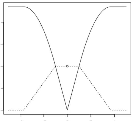
−4 −2 0 2 4 0.0 0.5 1.0 1.5 2.0 x y_penalty

Figure 2.1: SCAD penalty function (solid line) and its derivative (dotted line)

a

= 3

.

7

and

λ

= 1

zero automatically.

(c) Continuity, the estimator is continuous to avoid instability in model

pre-diction.

To achieve all the aforementioned three properties, Fan and Li (2001) proposed

the following so called SCAD penalty function,

P

(

|

β

|

) =























λ

|

β

|

,

|

β

| ≤

λ,

−

(

|

β

|

−

₂

_aλ

|

_β

|

₊

_λ

₎

_/

_[2(

_a

−

_1)]

_{, λ <}

|

_β

| ≤

_aλ,

(

a

+ 1)

λ

/

2

,

|

β

|

> aλ,

(2.6)

The important property for the SCAD penalty function is that it has the following

first derivative,

P

(

|

β

|

) =























λ,

|

β

| ≤

λ,

(

aλ

− |

β

|

)

/

(

a

−

1)

, λ <

|

β

| ≤

aλ,

0

,

|

β

|

> aλ,

for some

a >

2

.

(2.7)

function and its derivative are displayed in Figure 2.2.3. It can be clearly seen that

P

(

|

β

|

) is not differentiable at 0 with respect to

β

. Thus it is not easy to minimize the

penalized least squares functions due to its singularity. Fan and Li (2001) suggested

to approximate the penalty function by a quadratic function as

P

(

|

β

|

)

≈

P

(

|

β

|

) +

1

2

{

P

(

|

β

|

)

/

|

β

|}

(

β

−

β

)

for

β

≈

β

.

(2.8)

Alternatively, Zou and Li (2008) proposed local linear approximation (LLA) for

non-concave penalty functions as

[

P

(

|

β

|

)]

=

P

(

|

β

|

)sign(

β

)

≈ {

P

(

|

β

(0)

j

|

)

/

|

β

(0)

j

|}

β

,

(2.9)

which can reduce the computational cost without losing any statistical efficiency.

Recently, other algorithms such as mimorize-maximize (MM) algorithm are proposed

by Hunter and Li (2005).

Given a good initial value

β

such as maximal likelihood estimator (MLE)

without the penalty term, in view of (2.8), we can find the one-step estimator as

follow

β

= argmin

1

2

(

β

−

β

₎

_[

_−∇

_ℓ

₍

_β

_)](

_β

₋

_β

_{) +}

_n

∑

P

(

|

β

|

)

2

|

β

|

β

,

(2.10)

where

∇

_ℓ

₍

_β

_{) =}

_∂

_ℓ

₍

_β

0

)

/∂β∂β

. As argued in Fan and Li (2001), there is no

need to iterate until it converges as long as the initial estimator is reasonable. Also,

the MLE estimator from the full models without penalty term can be regard as the

reasonable estimator. For using the local linear approximation in Zou and Li (2008)

and (2.9), the sparse one-step estimator given in (2.10) becomes to

β

= argmin

1

2

(

β

−

β

₎

_[

_−∇

_ℓ

₍

_β

_)](

_β

₋

_β

_{) +}

_n

∑

P

(

|

β

|

)

|

β

|

β

.

(2.11)

As demonstrated in Zou and Li (2008), this one step estimator is as efficient as the

fully iterative estimator, provided that the initial estimator is good enough. For

example, we let

β

_{be the maximal likelihood estimator without the penalty term.}

2.3

Variable Selection for Covariates with Functional Coefficients

2.3.1

Notations and Technical Conditions

Let

{

(

X

, Z

, y

)

}

be a strictly stationary and strong mixing sequence, and

f

(

z, β

) be the density function of

z

=

β

_Z

_{, where}

_β

_{is an interior point of the compact}

set

B

. Define

A

=

{

Z

|

f

(

Z, β

)

≥

ε,

∀

β

∈

B

and

∃

a, b, β

Z

∈

[

a, b

]

}

as the domain

of

Z

, such that

β

Z

is bounded and the density of

f

(

Z, β

) is bounded away from

0. Also, define the domain of bandwidth

h

,

H

=

{

h

| ∃

C

and

C

, C

n

< h <

C

n

}

. For

Z

∈ A

∈

B

, and

h

∈ H

, define

n

by

p

matrix penalized estimator

as

b

G

(

b

β

)

=

[

b

g

(

b

β

Z

)

,

· · ·

,

b

g

(

b

β

Z

)]

= [

b

g

,

· · ·

,

b

g

]

,

where

b

g

(

b

β

Z

)

=

[

b

g

(

b

β

Z

)

,

· · ·

,

b

g

(

b

β

Z

)]

∈

R

,

and

b

g

=

[

b

g

(

ˆ

β

Z

)

,

· · ·

,

b

g

(

b

β

Z

)]

∈

R

.

Similarly, we can define true value

G

(

β

)

, g

(

β

Z

)

and

g

. Without loss of

gen-erality, we assume that first

p

functional coefficients are non-zero, and other

p

−

p

functional coefficients are zero, e.g.

∥

g

∦

= 0 and

g

are not constant everywhere

for 1

≤

k

≤

p

,

∥

g

∥

= 0 for

p

< k

≤

p

. Let

α

= max

{

P

(

∥

g

∥

) : 1

≤

k

≤

p

}

.

Then

α

= 0 as

n

→ ∞

. For an arbitrary matrix

X

= (

X

), we define

L

norm as

∥

X

∥

=

√∑

X

i,j

and the kernel function

K

=

K

(

x/h

)

/h

. Also we define object

function

Q

(

G,

b

β, h

ˆ

) =

∑

∑

{

y

−

b

g

(

ˆ

β

Z

)

X

}

K

(

ˆ

β

Z

−

β

ˆ

Z

)

+

n

∑

P

(

∥

b

g

∥

)

.

(2.12)

By minimizing the above object function with respect to ˆ

g

(

·

), one can obtain the

penalized local least squares estimator for

g

(

·

).

To study the asymptotic distribution of the penalized local least squares

esti-mator, we impose some technical conditions as follows.

(A1) The vector functions

g

(

·

) are bounded, not constant everywhere and have

con-tinuous second order derivatives with respect to the support of

A

.

(A2) For any

β

∈

B

and

Z

∈ A

, the density function

f

(

β

_Z

)

_{is continuous and}

there exists a small positive

ε

such that

f

(

β

Z

)

> ε

.

(A3) The kernel function

K

(

z

) is twice continuously differentiable on the support

(

−

1

,

1), Let

∫

z

_K

₍

_z

₎

_dz

₌

_µ

2

,

and

∫

K

₍

_z

₎

_dz

₌

_ν

0

.

(A4) lim

inf

P

n

(

θ

)

/λ

>

0,

n

_λ

→

0,

h

∝

n

and

∥

β

ˆ

−

β

∥

=

Op

(1

/

√

n

).

(A5) Define Ω

(

β

_Z

)

₌

_E

(

_X

X

|

β

Z

)

, Ω

(

β

_Z

)

_{is nonsingular and has bounded}

second order derivative on

A

.

(A6)

{

(

Xi, Zi, yi

)

}

is a strictly stationary and strongly mixing sequence with mixing

coefficient

α

(

m

) =

O

(

ρ

_{) for some 0}

_{< ρ <}

_1.

(A7) Let

z

=

β

_Z

_{, the conditional density}

_f

₍

_z

i

, z

|

z

) is continuous and has bounded

second order derivative.

(A8) Let Ω (

z

, z

, z

) =

E

(

X

X

X

X

|

z

, z

, z

)

be continuous and has bounded

sec-ond order derivative. Define Ω (

z

, z

, z

) = Ω (

z

, z

, z

)

|

,

Ω

(

z

, z

, z

)

=

∂

Ω (

z

, z

, z

)

/∂z

and Ω

(

z

, z

, z

) =

∂

Ω (

z

, z

, z

)

/∂z

.

Remark 2:

The conditions in A2 imply that the distances between two ranked

val-ues

β

Z

are at most order of

Op

(log

n/n

) (Janson 1987). For any value Λ

∈ A

,