Partition Models for Variable Selection and Interaction Detection

(1)

Partition Models for Variable Selection and Interaction Detection

(Article begins on next page)

The Harvard community has made this article openly available.

Please share

how this access benefits you. Your story matters.

Citation

Jiang, Bo. 2013. Partition Models for Variable Selection and

Interaction Detection. Doctoral dissertation, Harvard University.

Accessed

April 17, 2018 4:06:05 PM EDT

Citable Link

http://nrs.harvard.edu/urn-3:HUL.InstRepos:11124828

Terms of Use

This article was downloaded from Harvard University's DASH

repository, and is made available under the terms and conditions

applicable to Other Posted Material, as set forth at

http://nrs.harvard.edu/urn-3:HUL.InstRepos:dash.current.terms-of-use#LAA

(2)

Partition Models for Variable Selection and Interaction

Detection

A dissertation presented by Bo Jiang to

The Department of Statistics in partial fulfillment of the requirements

for the degree of Doctor of Philosophy in the subject of Statistics Harvard University Cambridge, Massachusetts April 2013

(3)

c 2013 - Bo Jiang

(4)

Professor Jun S. Liu Bo Jiang

Partition Models for Variable Selection and Interaction Detection

Abstract

Variable selection methods play important roles in modeling high-dimensional data and are key to data-driven scientific discoveries. In this thesis, we consider the problem of variable selection with interaction detection. Instead of building a predictive model of the response given combinations of predictors, we start by modeling the conditional distribution of pre-dictors given partitions based on responses. We use this inverse modeling perspective as motivation to propose a stepwise procedure for e↵ectively detecting interaction with few assumptions on parametric form. The proposed procedure is able to detect pairwise interac-tions amongppredictors with a computational time ofO(p) instead ofO(p2_{) under moderate}

conditions. We establish consistency of the proposed procedure in variable selection under a diverging number of predictors and sample size. We demonstrate its excellent empirical performance in comparison with some existing methods through simulation studies as well as real data examples.

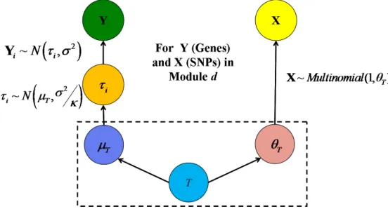
Next, we combine the forward and inverse modeling perspectives under the Bayesian framework to detect pleiotropic and epistatic e↵ects in e↵ects in expression quantitative loci (eQTLs) studies. We augment the Bayesian partition model proposed by Zhang et al. (2010) to capture complex dependence structure among gene expression and genetic markers. In particular, we propose a sequential partition prior to model the asymmetric roles played by the response and the predictors, and we develop an efficient dynamic programming

(5)

algo-rithm for sampling latent individual partitions. The augmented partition model significantly improves the power in detecting eQTLs compared to previous methods in both simulations and real data examples pertaining to yeast.

Finally, we study the application of Bayesian partition models in the unsupervised learn-ing of transcription factor (TF) families based on protein bindlearn-ing microarray (PBM). The problem of TF subclass identification can be viewed as the clustering of TFs with variable selection on their binding DNA sequences. Our model provides simultaneous identification of TF families and their shared sequence preferences, as well as DNA sequences bound pref-erentially by individual members of TF families. Our analysis may aid in deciphering cis

(6)

Acknowledgments

This dissertation would not have been possible without the support of many people. I am most grateful to my advisor, Professor Jun S. Liu, for his continuous encouragement and support throughout my years at Harvard. It has been my privilege to have him as a mentor in both academic research and personal life. I thank Professor Joseph Blitzstein and Professor Martha Bulyk for serving on my dissertation committee and providing many invaluable comments on my thesis writing. Professor Martha Bulyk has been a long time collaborator who guided me in the protein binding microarray project. I sincerely appreciate her patience in revising my paper word by word and broadening my scientific knowledge. I would also like to thank National Science Foundation, National Institute of Health and National Human Genome Research Institute for supporting my research with Professor Jun S. Liu and Professor Martha Bulyk through NSF grant 1007762 and NIH/NHGRI R01 HG003985.

Throughout my years at Harvard, it has been my distinct honor to serve as teaching fellows for Professor Joseph Blitzstein, Professor Stephen Blyth and Professor Xiao-Li Meng, who helped me develop various teaching skills and treated me with both food of statistics and food of stomachs. I also thank all the faculty and sta↵members in the statistics department for providing an incredible learning environment and supportive statistical community.

The long journey of graduate study would be miserable without friends and classmates. I thank Alex Blocker, Ke Deng, Valeria Espinosa, Daniel Fernandez, Simeng Han, Jonathan Hennessy, Ming Hu, Roee Gutman, Joseph Kelly, Yang Li, Cli↵Meyer, Nathan Stein, Samuel Wong, Jiexing Wu, Thomas Xiao, Xianchao Xie (a.k.a “XX”), Xiaojin Xu, Yuan Yuan, Anqi

(10)

Zhao and Li Zhu for their support, friendship and wisdoms. I also very much enjoyed the companions of undergraduate concentrators, Raj Bhuptani, Jessica Hwang and Keli Liu, who have been my students, TF-mates and teachers.

Last but not least, I owe my greatest gratitude to my parents, Jinhai Jiang and Ru Wang, and my wife, Huayue Zhang, for their love and support. They always encouraged me to pursue what I want and make best e↵orts to make it happen.

(11)

(12)

Chapter 1

Introduction

Recently there has been a significant surge of interest in analytically accurate, numerically robust, and algorithmically efficient variable selection methods, largely due to the tremen-dous advance in data collection techniques such as those in genetics, internet, and marketing. The importance of discovering truly influential factors from a large pool of possibilities is now widely recognized by both general scientists and quantitative modelers. Motivated by di↵ er-ent scier-entific applications, developmer-ents of variable selection techniques encompass various dimensions of statistical modeling including:

• Parametric versus nonparametric models. When a specific form can be derived from solid scientific arguments, parametric models are more accurate in making predic-tions. In other cases, nonparametric models are more flexible and robust to model mis-specifications, especially in the stage of variable screening and data exploratory analysis. In practice, nonparametric procedures usually involve choosing a discretiza-tion (or partidiscretiza-tion) scheme of continuous data, reflecting a bias-variance trade-o↵ on the resolution of our model assumptions.

(13)

• Univariate versus multivariate responses. While it is straightforward to regress each univariate component onto predictors separately, a joint model of multiple responses can reveal relationships among responses and aggregate information from correlated responses to improve the signal strength in selecting important predictor variables. • Supervised versus unsupervised learning problems. In supervised learning problems,

such as classification and regression, the inclusion of redundant variables in the learning procedure may degrade the results. Similarly, in clustering, or unsupervised learning problems, the structure of interest may be best represented using only a few of the feature variables and some form of variable selection prior to, or incorporated into the fitting procedure is advisable.

• Frequentist versus Bayesian approaches. Frequentist methods usually enjoy computa-tional simplicity and asymptotic properties such as consistency. On the other hand, Bayesian framework provides a coherent way to take into account prior knowledge and uncertainties in model selection. Variable selection strategies have benefited from both Frequentist and Bayesian ideas and the interplay of the two standpoints continues to inspire the development of new methods.

In this thesis, we will explore an additional dimension in statistical modeling for variable selection, the forward versus inverse modeling perspective, which leads to the development of partition models for several applications.

(14)

1.1

An Overview of Variable Selection Methods

Under linear regression models, various regularization methods have been proposed for simultaneously estimating regression coefficients and selecting predictors. Many promising algorithms, such as Lasso (Tibshirani, 1996; Zou, 2006; Friedman et al., 2007), LARS (Efron et al., 2004) and smoothly clipped absolute deviation (SCAD) (Fan and Li, 2001), have been invented. When the number of predictors is extremely large, Fan and Lv (2008) have proposed a sure independence screening (SIS) framework that first independently selects variables based on their correlations with the response and then applies variable selection methods in the second step.

When the relationship between the response Y and predictors X = (X1, X2, . . . , Xp)T is

beyond linear, the performance of the variable selection methods based on the linear model assumption can be severely compromised. In his seminal paper on dimension reduction, Li (1991) proposed a semi-parametric index model of the form

Y =f( T1X, 2TX, . . . , TqX,✏), (1.1)

wheref is an unknown link function and✏is a stochastic error independent ofX. A sliced in-verse regression (SIR) method was developed by Li (1991) to estimate the so-called sufficient dimension reduction (SDR) directions ₁, . . . , _q. Since the estimation of SDR directions does not automatically lead to variable selection, various methods have been developed to perform dimension reduction and variable selection simultaneously in the nonlinear setting. For example, Li (2007) developed sparse SIR (SSIR) algorithm to obtain shrinkage estimates of the SDR directions under L1 norm. Zhong et al. (2012) proposed a stepwise procedure called correlation pursuit (COP) for index models under the SIR framework.

(15)

The number of variables to be considered can be even larger with the inclusion of inter-action terms between predictors. Consider the following simple example with a regression model for a univariate response variableY andpindependent normally distributed predictor variables X= (X1, X2, . . . , Xp)T,

Y =X1X2+ 0.1✏, (1.2)

where X_⇠MVNp(0,Ip) and ✏⇠N(0,1). For illustrative purpose, we add a relatively small

noise term 0.1✏ here. Since there are p₂ pairwise interactions, fitting regression models with 2-way interactions using variable selection methods, or even the sure independence screening procedure, is challenging when one has a moderate number of predictor variables, say p = 1000. Recently, there has been considerable e↵ort in fitting interaction models in the statistical literatures. For example, Bien et al. (2012) developed hierNet, an extension of Lasso to consider interactions in a model if one or both variables are marginally important (referred to as hierarchical interactions by the authors). Li et al. (2012) proposed a sure independence screening procedure based on distance correlation (DC-SIS) that is shown to be capable of detecting important variables when interactions are presented.

1.2

Forward versus Inverse Modeling Perspectives

Most of the aforementioned methods are derived from a forward modeling perspective, that is, a model for the conditional distribution of Y given X. When predictor variables

X can be treated as random, we obtain a di↵erent modeling perspective by “flipping” the roles of X and Y and putting the response Y behind the (conditioning) bar, which we call an inverse model. Indeed, this inverse modeling perspective has been taken by several

(16)

researchers and has led to new developments in dimension reduction and variable selection methods. Cook (2007) proposed inverse regression models for dimension reduction, which have deep connections with the SIR method. Simon and Tibshirani (2012) proposed a permutation-based method for testing interactions by exploring the connection between the

forward logistic model and theinverse normal mixture model when the responseY is binary. Another classical method derived from the inverse modeling perspective is the Na¨ıve Bayes classifier for classifications with high-dimensional features. Although Na¨ıve Bayes classifier is limited by its strong independence assumption, it can be generalized by modeling the joint distribution of features. Murphy et al. (2010) proposed a variable selection method using Bayesian information criterion (BIC) for model-based discriminant analysis. Zhang and Liu (2007) proposed a Bayesian method called BEAM to detect epistatic interactions in genome-wide case-control studies, where Y is binary and X are discrete.

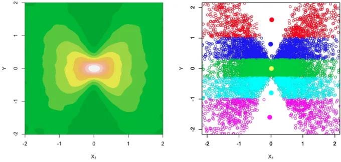
The inverse modeling perspective can also shed lights on interaction detections. Figure 1.1 shows the contour plot for the joint distribution of Y and X1 from the example in (1.2). If we divide the response into five slices and calculate the mean and variance ofX1 within each slice (as shown in Figure 1.1), we can see that although X1 is marginally uncorrelated with

Y and the conditional means ofX1are the same, the conditional variances ofX1 across slices are very di↵erent. Instead of screening all the p₂ =O(p2_{) pairwise interaction terms, we can}

discover the importance ofX1 andX2 by examining the conditional variances ofpindividual predictors given the sliced response, which only requires a computational complexity ofO(p). Motivated by this observation, in this thesis we investigate an inverse modeling approach to attack the problem of interaction detection without imposing model-specific assumptions on the relationship between the response and predictors.

(17)

Figure 1.1: Left panel: contour plot for the joint density of Y and X1 in the example (1.2). Right panel: conditional means and variances ofX1 given slices ofY. Slices are indicated by di↵erent colors and round dots mark the conditional means of X1 across slices. The sample

conditional variances ofX1 within di↵erent slices (from top to bottom) are: 2.29, 0.92, 0.41, 0.98 and 2.33.

1.3

Integrating Two Perspectives with Partition Model

In Chapter 2, we propose a statistical model for variable selection with interaction detec-tion under the sliced inverse regression framework. A stepwise procedure based on likelihood-ratio test, which we refer to as SIRI, is developed to select relevant predictors from a inverse modeling perspective. Frequentist properties of the proposed variable selection procedure are established and, in particular, its asymptotic behavior under a diverging number of pre-dictors and sample size is investigated. Although the proposed procedure shows promising performance in comparison with existing methods in both simulation studies and real data examples, there are several limitations: (1) the choice of fixed slicing scheme is rather ad hoc; (2) stepwise variable selection methods tend to miss important predictor with weak marginal but strong joint e↵ects; (3) there is no straightforward generalization to model

(18)

multiple responses and their correlations. These limitations motive us to seek a Bayesian analogue of the slice inverse regression framework.

Under a Bayesian framework, we generalize the concept of slice by introducing a latent variableT that we call individual type. Conditioning on individual type T, we first decouple the forward and inverse perspectives by temporarily releasing both X and Y out of the (conditioning) bar and modeling them separately. Then, we combine both models to draw posterior inferences on T given its prior distribution. The question that remains is how best to model hidden individual type T. The Dirichlet process prior, a common choice in unsupervised Bayesian clustering, is flexible but not suitable for modeling individual types in regression problems. Since our objective here is to extract information from predictorsX

that can be used to explain variation in the response Y, the Dirichlet process prior gives X

and Y too much “freedom” and does not respect the asymmetric roles played by X and Y. To accommodate the objective of supervised learning, in Chapter 3, we propose a sequential partition prior for modeling individual typeT and an efficient sampling algorithm based on dynamic programming.

1.4

Applications in Genetics and Gene Transcriptional

Regulations

Developments of statistical models and variable selection methods in this thesis are moti-vated by genetic studies in expression quantitative trait loci (eQTL) and biological research in gene transcriptional regulation.

Expression quantitative trait loci (eQTLs) are genomic loci that regulate expression levels of genes. By assaying gene expression and genetic variation simultaneously on a

(19)

genome-wide basis, scientists wish to discover groups of genomic loci (among millions) that can a↵ect the expression of a subset of genes (among thousands). The problem can be viewed as a multivariate regression with variable selection on both responses (gene expression) and pre-dictors (genetic markers), including also multi-way interactions among correlated prepre-dictors (called epistatic e↵ects of genetic markers). Motivated by BEAM model (Zhang and Liu, 2007) for genome-wide case-control studies, Zhang et al. (2010) proposed a Bayesian par-tition model for eQTL studies with continuous responses (expression levels of genes) and discrete predictors (genotypes of genetic markers).

Transcription factors (TFs) regulate the expression of their target genes through interac-tions with specific DNA binding sites in the genome. In our e↵ort to generalize the partition model to identify key regulatory TFs in embryonic stem cells, when both the response (gene expression) and predictors (TF binding specificities) are continuous, we found interesting links with sliced inverse regression (SIR) and correlation pursuit (COP) that finally lead to the development of a procedure for detecting interactions from an inverse modeling per-spective, which we named SIRI in Chapter 2. The proposed procedure can be viewed as a Frequentist analogue of the Bayesian partition model (Zhang et al., 2010) for continuous response and predictor variables.

TFs with similar structures can be divided into subclasses, with more closely related pro-teins exhibiting more similar DNA binding preferences. Numerous studies have employed universal protein binding microarray (PBM) (Berger et al., 2006) technology to determine the in vitro binding specificities of hundreds of TFs for all possible 8-bp DNA sequences (8-mers). Identification of TF subclasses based on PBM 8-mer data can be viewed as an unsupervised learning (clustering) problem with variable selections. In Chapter 4, we gen-eralize the Bayesian partition model to provide simultaneous identification of TF subclasses

(20)

and their shared sequence preferences, and also of 8-mers bound preferentially by individual members of TF subclasses. Such results may aid in deciphering cis regulatory codes and determinants of protein-DNA binding specificity.

The development of SIRI and its application in transcriptional regulation also provide new research ideas on improving the partition model for eQTL studies. Inspired by a dynamic slicing scheme designed for SIRI, we propose a sequential partition prior, which accounts for the asymmetric roles played by response and predictors in eQTL problems, and develop an efficient dynamic programming algorithm for sampling latent individual partitions in Chap-ter 3. We further augment the Bayesian partition model to capture complex dependence structure among gene expression and genetic markers, especially negative co-expression be-tween genes and linkage disequilibrium (LD) bebe-tween genetic markers. Through simulation studies and a real data example in yeast, we demonstrate how the augmented Bayesian partition model achieved significantly improved power in detecting eQTLs compared to the original model proposed by Zhang et al. (2010) and other traditional methods.

1.5

Outline

An outline for the remainder of this dissertation is as follows. Chapter 2 gives a detailed account of the SIRI method for variable selection and interaction detection with comparisons and connections to previous methods. Chapter 3 elaborates the Bayesian partition model and its extension for identifying pleiotropic and epistasis eQTLs. Chaper 4 studies the application of partition model in unsupervised learning of TF subclasses based on PBM

(21)

Chapter 2

Sliced Inverse Regression with

Interaction Detection

LetY ₂Rbe a univariate response variable andX= (X1, X2, . . . , Xp)T 2Rp be a vector

of p continuous predictor variables with covariance matrix ⌃p = Cov (X). {(xi, yi)}ni=1 are

independent observations of (X, Y). For discrete response, we can naturally group _{yi}ni=1

into a finite number of classes. For continuous response, the range of _{yi}ni=1 can be divided

intoH disjoint intervals, referred to as slices, which are denoted asS1, S2, . . . , SH. We define

a random variableS(Y) as the slice membership of responseY, that is, S(Y) =h ifY ₂Sh.

For a fixed slicing scheme, we denote nh =|Sh|=shn where PH_h₌₁sh = 1.

The working model of the sliced inverse regression (SIR) method is given by (1.1). After standardization, Z=⌃ 12

p [X E(X)], we can rewrite model (1.1) as

Y =f ⌘T₁Z,⌘T₂Z, . . . ,⌘T_qZ,✏ with ⌘_i =⌃12

p i. (2.1)

(22)

al-gorithm was motivated by the following observation: under model (2.1), ifE bT_Z_|_⌘T

1Z, . . . ,⌘TqZ

is linear in⌘T

1Z, . . . ,⌘TqZ for any vectorb2Rp, then E(Z|Y) is contained in the linear

sub-space spanned by ⌘₁, . . . ,⌘_q (Li, 1991). So if the firstq largest eigenvalues of Cov (E(Z_|Y)) are all positive, SDR directions can be obtained by the corresponding eigenvectors.

Eigenvalues of Cov (E(Z_|Y)) also connect SIR with multiple linear regression (MLR). In MLR, the correlation squared, R2, can be defined as

R2 = max

b2Rp

⇥

Corr Y,bTZ ⇤2,

while in SIR, the largest eigenvalue of Cov (E(Z_|Y)), called the firstprofile-R2_{, can be defined}

as

1(Cov (E(Z|Y))) = max

b2Rpmax_T

⇥

Corr T(Y),bTZ ⇤2,

where the maximum is taken over all bounded transformationsT(·) and vectorsb 2Rp_(Chen

and Li, 1998). We can further define the kth profile-R2_,

k (2 k  q), as the kth largest

eigenvalue of Cov (E(Z|Y)) by restricting the vector b to be orthogonal to eigenvectors of the first (k 1) profile-R2_{. Building upon this connection with MLR, Zhong et al. (2012)}

proposed the correlation pursuit (COP) method for variable selection motivated by the F-test in stepwise regression. The COP statistic is defined as

COPd_k+1 =nb d+1 k bdk 1 bd_k+1 , k= 1,2, . . . , q, and COP d+1 1:q = q X k=1 COPd_k+1, wherebd

kandbdk+1 are thekth profile-R2estimated from the current set of selected predictors

of dimension dand current selected predictors plus an additional predictor to be considered, respectively. A stepwise procedure based on the COP statistic was developed in Zhong et al.

(23)

(2012) for simultaneous dimension reduction and variable selection.

2.1

From SIR to SIRI: An Inverse Model for Variable

Selection and Interaction Detection

To take an inverse perspective on SIR, we start with a seemingly di↵erent model. We assume that the distribution of predictors given the sliced response is multivariate normal:

X|Y 2Sh ⇠MVN (µh,⌃),1h H, (2.2)

where µh µ 2Vq belongs to a q-dimensional affine space, Vq is a q-dimensional subspace

(q < p) and µ₂Rp_{. Alternatively, we can write} _µ

h =µ+ h, where h 2 Rq and is a p

byq matrix whose columns form a basis of the subspaceVq_{. Although this representation is}

only unique up to a orthonormal transformation on the bases , the subspace Vq _{is unique}

and identifiable. The following proposition proved by Szretter and Yohai (2009) links the inverse model (2.2) with SIR.

Proposition 1. The maximum likelihood estimate (MLE) of the bases of subspace Vq _in

model (2.2) coincides with the SDR directions estimated from the SIR algorithm up to a orthonormal transformation.

According to Proposition 1, we could have derived the SIR algorithm from an inverse model. Next, we propose to select variables via a hypothesis testing framework based on this model.

(24)

2.1.1

Likelihood-Ratio Tests for Selecting Variables with Marginal

E

↵

ects

Here we provide a view of the COP method for selecting variables with marginal e↵ects from an inverse modeling perspective. This will lay the ground work for the augmented model to select variables with interaction e↵ects in the next section.

For the purpose of variable selection, we partition predictors into two subsets: a set of relevant predictors indexed by A and a set of redundant predictors indexed by Ac_{, and}

assume the following model:

X_A|Y 2Sh ⇠ MVN (µh 2µ+Vq,⌃), (2.3)

X_Ac|X_A, Y 2S_h ⇠ MVN ↵+ TX_A,⌃₀ .

That is, we assume that the conditional distribution of relevant predictors follows the inverse model (2.2) of SIR and has a common covariance matrix in di↵erent slices. Given the current set of selected predictors indexed by C with dimension d and another predictor indexed by

j /2C, we propose the following hypotheses:

H0 :A =C v.s. H1 :A=C[{j}.

Let ⇥0 and ⇥1 denote the parameter space under H0 and H1, respectively. The

likelihood-ratio test statistic can be written as

L_j|C = max✓12⇥1(P✓1(X|Y)) max✓02⇥0(P✓0(X|Y)) = Pb✓1 X[C[{j}]c|Xj,XC, Y Pb✓1(Xj|XC, Y) Pb✓0 X[C[{j}] c|X_j,X C, Y Pb✓0(Xj|XC, Y) = P✓b0(Xj|XC, Y) P✓b0(Xj|XC, Y) ,

(25)

where ✓b0 = argmax✓02⇥0(P✓0(X|Y)), b✓1 = argmax✓12⇥1(P✓1(X|Y)), and the last equality

follows from P_✓_b₁ X[C[{j}]c|Xj,XC, Y = Pb✓0 X[C[{j}]c|Xj,XC, Y according to model (2.3).

The scaled log-likelihood-ratio test statistic is given by

b Dj|C = 2 n log Lj|C = q X k=1 log 1 + b d+1 k bdk 1 bd+1 k ! , (2.4) where bd

k and bdk+1 are estimates of the kth profile-R2 based on xC and xC[{j}, respectively.

Under the null hypothesis, bdk+1 bdk

1 bd_k+1

P

!0. Since log(1 +t)_⇡t when t is small, we have

⇣ nDbj|C ⌘ _P !COPd_1:+1_q = q X k=1 COPd_k+1 !D 2 q,

asn_{! 1}. Coincidentally, we re-discovered the COP statistic of Zhong et al. (2012) from an inverse model. For all the predictors indexed by j ₂ _Cc_{, we can also obtain the asymptotic}

joint distribution of ⇣nDbj|C

⌘

under the null hypothesis:

⇣ nDbj|C ⌘ j2Cc D ! K X k=1 z_kj2 ! j2Cc (2.5) where zk= (zkj)_j₂_Cc ⇠MVN ⇣ 0,[Corr (Xi, Xj|XC)]i,j2Cc ⌘

and zk’s are independent.

Furthermore, as n _{! 1},

b

D_j|C a.s._!D_j|C = log 1 + Var(Mj) Cov (Mj,XC) [Cov (XC)]

1

Cov (Mj,XC)T

Vj

!

where Mj = E(Xj|XC, S(Y)), Vj = Var (Xj|XC, S(Y)) and S(Y) = h when Y 2 Sh (1 

(26)

Cauchy-Schwarz inequality and normality assumption,

Dj|C = 0 i↵ E(Xj|XC, Y 2Sh) =E(Xj|XC),1hH.

That is, the test statisticDbj|C almost surely converges to zero if the conditional mean of Xj

is independent of slice membership S(Y). Detailed proofs on properties of likelihood-ratio test statistic are delegated to Appendix A.1.

Given thresholds ⌫a >⌫d and the current set of selected predictors indexed by C, we can

select relevant variables by iterating the following steps until no new addition or deletion occurs:

• Addition step: find ja such that Dbja|C = maxj2CcDbj|C; ifDbja|C >⌫a, let C =C+{ja}. • Deletion step: find jd such that Dbjd|C {jd} = minj2CDbj|C {j}; if Dbjd|C {jd} < ⌫d, let

C =_C _{jd}.

Under model (2.3), for relevant predictors indexed by j 2A, we have

Xj|XA {j}, Y 2Sh ⇠N ⇣ ↵(_jh)+ T_jX_{A {}j}, j2 ⌘ ,1_h_H. (2.6) Let↵j(Y) = PHh=1↵ (h)

j I(Y 2Sh). We introduce the following concept to study the marginal

e↵ect of relevant predictors.

Definition 1 (Marginally Detectable). We say a predictor indexed by j is marginally de-tectable if there exist constants  0 and ⇠>0 such that

(27)

for all n.

Under the following conditions, the stepwise procedure proposed above is consistent by choosing the thresholds appropriately.

Condition 1. There exist 0<⌧min<⌧max <1 such that

⌧min min(Cov (X|Y 2Sh))< max(Cov (X|Y 2Sh))⌧max,

and

max(Cov (X))⌧max,

where min(·) and max(·) denote the smallest and largest eigenvalue of a positive definite

matrix.

Condition 2. p = O(n⇢₎ _as _n _{! 1} _with _⇢ _> ₀ _and ₂_⇢_{+ 2}_ _< ₁_{, where} _ _{is the same} constant as in (2.7).

The following theorem is proved in Appendix A.2.

Theorem 1. Under Condition 1 and Condition 2, if all the relevant predictors indexed by

A in model (2.3) are marginally detectable with constant , then there exists constant c >0

such that Pr ✓ min C:Cc_\_A_6=;max_j₂_Cc Dbj|C cn  ◆ !1, and Pr ✓ max C:Cc_\_A_=;max_j₂_Cc Dbj|C < c 2n  ◆ !1, as n ! 1.

Thus, if we choose the threshold ⌫a =cn  and ⌫d = (c/2)n  with c and  defined above,

(28)

been included, and once all the relevant predictors have been included, all the redundant variables will be removed from the selected variables.

2.1.2

An Augmented Model with Interaction Detection

Let us revisit the simple example in (1.2) with the stepwise procedure based on the likelihood-ratio test statistic proposed in the previous section. In this example,E(X1|Y 2Sh) =

E(X2|Y 2Sh) = 0 for 1hH. In the first addition step with C =;, the stepwise

proce-dure fails to capture eitherX1 orX2 sinceD1_|C=; =D2|C=; = 0. In order to detect predictors

with interactions, such as X1 and X2 in this example, we augment model (2.3) to a more general form:

X_A|Y 2Sh ⇠ MVN (µh,⌃h), (2.8)

X_Ac|X_A, Y 2S_h ⇠ MVN ↵+ TX_A,⌃₀ ,

which di↵ers from model (2.3) in its allowing for slice-dependent means and covariance matrices for relevant predictors.

Under model (2.8), a predictor indexed by j 2 A is conditionally irrelevant if the con-ditional distribution of Xj given XA {j} and S(Y) does not depend on slice S(Y). If there

exists a conditionally irrelevant predictor indexed byj 2A, then we can always redefine the index set of relevant predictors to be A {j} in model (2.8). To guarantee identifiability, variables indexed byAin model (2.8) have to beminimally relevant, that is,Adoes not con-tain any conditionally irrelevant predictor. For example, if the joint distribution of (X1, X2) depends onS(Y) and all the other variables are conditionally independent ofS(Y) givenX1, then X3 is conditionally irrelevant given (X1, X2) and so {X1, X2, X3} is relevant but not

(29)

minimally relevant. In this example, _{X1, X2} is minimally relevant if both the conditional

distribution ofX1 givenX2 and the conditional distribution ofX2 givenX1 depend on S(Y).

In Appendix A.3, we prove the following proposition:

Proposition 2. The set of minimally relevant predictors indexed by _A under model (2.8) is unique given Condition 1.

By following the same hypothesis testing framework for variable selection in the previous section, we can derive the scaled log-likelihood-ratio test statistic under the augmented model (2.8): b D_j⇤_|C = log_b2_j H X h=1 nh n log h b(jh) i2 , (2.9)

where C indexes currently selected predictors and j 2 Cc_, h_b(h) j

i2

is the estimated variance by regressing Xj onXC in slice Sh, andbj2 is the estimated variance by regressing Xj onXC

using all the observations. Under the assumption that A ⇢ C with |C| = d, we can derive the exact and asymptotic distribution of ⇣nDb⇤

j|C ⌘ : nDb⇤_j|C ⇠nlog 1 + _P_HQ0 h=1Qh ! _H X h=1 nh n log Qh/nh PH h=1Qh/n ! D ! 2 (H 1)(d+2), whereQ0 _⇠ 2

(H 1)(d+1)andQh ⇠ n2h (d+1)(1hH) are mutually independent according to Cochran’s theorem. For all the predictors indexed by j ₂ _Cc _{given predictors indexed by}

C, we can also obtain the asymptotic joint distribution of ⇣nDb⇤

j|C

⌘

under the assumption that _A_⇢_C: ⇣ nDb⇤_j_|C⌘ j2Cc D ! 0 @ (H _X1)(d+1) i=1 z_ij2 + H_X1 i=1 e z_ij2 1 A j2Cc , (2.10)

(30)

where zi’s andezi’s are mutually independent with zi = (zij)_j₂_Cc ⇠MVN ⇣ 0,[Corr (Xj, Xk|XC)]j,k2Cc ⌘ , and ezi = (zeij)_j₂_Cc ⇠MVN ⇣ 0,⇥Corr2(Xj, Xk|XC) ⇤ j,k2Cc ⌘ . We have, as n ! 1, b D⇤_j|C a.s.!D_j|C⇤

= log 1 + Var(Mj) Cov (Mj,XC) [Cov (XC)]

1

Cov (Mj,XC)T

E(Vj)

!

+ logE(Vj) Elog (Vj),

where Mj = E(Xj|XC, S(Y)), Vj = Var (Xj|XC, S(Y)) and S(Y) = h when Y 2 Sh (1 

h_H). According to the Cauchy-Schwarz inequality and Jensen’s inequality,

for 1  h  H. That is, the augmented test statistic Db_j⇤_|C almost surely converges to zero if both the conditional mean and the conditional variance of Xj is independent of slice

membership S(Y). Proofs on properties of the augmented likelihood-ratio test statistic are delegated to Appendix A.4.

A forward-addition backward-deletion algorithm similar to the stepwise procedure pro-posed in Section 2.1.1 can be used with the augmented likelihood-ratio test statistic Db⇤_j_|C. To investigate the power of the augmented likelihood-ratio test, we introduce the following

(31)

concepts.

Definition 2 (Conditionally Detectable). We say a collection of predictors indexed by _C2 is conditionally detectable given predictors indexed by _C1 if C2\C1 = ;, and for any set C satisfying _C1 ⇢C and C2 6⇢C, there exist constants  0, ⇠1,⇠2 >0 such that either

max

j2Cc_\_C₁

"

Var(Mj) Cov(Mj,XC) [Cov(XC)] 1Cov(Mj,XC)T

E(Vj) # ⇠1n , (2.11) or max j2Cc_\_C₁[log (EVj) Elog (Vj)] ⇠2n  where Mj =E(Xj|XC, S(Y)), Vj =Var(Xj|XC, S(Y)).

In other words, if the current selection _C contains _C1, then there always exist detectable

predictors conditioning on currently selected variables until we include all the predictors indexed by _C2. A relevant predictor Xj indexed by j /2 C2 is not conditionally detectable

given _C1 either because it is highly correlated with some other predictors, or its e↵ect can

only be detected when conditioning on predictors that have not been included in _C1. Based

on Definition 2, we define stepwise detectable recursively as following.

Definition 3 (Stepwise Detectable). A collection of predictors indexed by T0 is said to be

0-level detectable if X_T0 is conditionally detectable given an empty set, and a collection of

predictors indexed by Tm is said to be m-level detectable (m 1) if XTm is conditionally

detectable given predictors indexed by [m 1

i=1 Ti. Finally, a predictor indexed by j is said to be

stepwise detectable if j 2 [1

i=1Ti.

According to Lemma 1 in Appendix A.2, given the same constant , there exists ⇠1 such that the set of marginally detectable predictors defined in Definition 1 is contained inT0, the

(32)

set of 0-level detectable predictors. As a result, the definition of stepwise detectable expand the concept of marginally detectable. In Appendix A.5, we will show that by appropriately choosing thresholds, the stepwise procedure will keep adding predictors until all the stepwise detectable predictors have been included.

A in model (2.3) are stepwise detectable with constant , then there exists constant c⇤ _>₀ such that as n _{! 1}, Pr ✓ min C:Cc_\_A₆₌_;max_j₂_Cc Db ⇤ j|C c⇤n  ◆ !1, and Pr ✓ max C:Cc_\_A₌_;max_j₂_Cc Db ⇤ j|C < c⇤ 2n  ◆ !1.

Thus, by appropriately choosing the thresholds, the stepwise procedure based on Db⇤

j|C is

consistent in identifying stepwise detectable predictors.

2.1.3

A Sure Independence Screening Strategy

When the dimensionalitypis extremely large (e.g., exceedingn2_{), the performance of the}

stepwise procedure can be compromised. Therefore, we recommend adding an independence screening step to first reduce the dimensionality from ultra-high to moderately high. A natural choice of test statistic for the independence screening procedure is Db⇤

j =Db⇤j|C with

C = _;, that is, the augmented likelihood-ratio test statistic used in the first addition step of the stepwise procedure. If we rank predictors according to _{Db⇤

j,1 j  p}, then a sure

independence screening (SIS) procedure that takes the first n 1 or n/log(n) predictors has a high probability (almost surely) of including the independently detectable predictors defined below.

(33)

Definition 4(Independently Detectable). We say a predictorXj is independently detectable

if there exist constants  0 and ⇠1,⇠2 such that either

Var(E(Xj|S(Y)))

E(Var(Xj|S(Y)))

⇠1n , (2.12)

or

logE(Var(Xj|S(Y))) Elog [Var(Xj|S(Y))] ⇠2n .

Simply put, independently detectable predictors have either di↵erent means or di↵erent variances across slices. Therefore, in the example (1.2), both X1 and X2 are independently detectable because Var(X1|Y 2 Sh) and Var(X2|Y 2 Sh) (1  h  H) are di↵erent across

slices.

In Theorem 3, we proved that the SIS procedure based on {Dbj⇤,1  j  p} almost

surely includes the independently detectable predictors under the following condition with ultra-high dimensionality of predictors.

Condition 3. log(p) = O(n ) as n! 1 with0< + 2<1, where  is the same constant as in (2.12). Furthermore, the number of the relevant predictors |A| ⇠0n⌘ with ⌘+<1

and constant ⇠0 >0.

We prove the following theorem in Appendix A.6.

A are independently detectable, then there existc > 0 and C >0 such that

Pr ✓ min j2ADb ⇤ j cn  ◆ !1,

(34)

and

Pr⇣_{j :Db⇤_j cn _,₁__j __p_} __Cn+⌘⌘_!₁_.

According to Theorem 3, we can first use the SIS procedure to reduce the dimensionality from

pto a scale below sample size, sayn/log(n), and then apply the stepwise procedure proposed in the previous sections. Note that predictors that are marginally or stepwise detectable according to Definition 1 and Definition 3 are not necessarily independently detectable. Fan and Lv (2008) advocated an iterative procedure that alternates between a large-scale screening and a moderate-scale variable selection to enhance the performance, which will be discussed in the next section.

2.2

Cross-Stitching and Cross-Validation

The simple model (2.3) and the augmented model (2.8) compensate each other in terms of the bias-variance trade-o↵. Given finite observations, model (2.3) is simpler and more powerful when the response is driven by some linear combinations of predictors, while model (2.8) is useful in detecting more complex relationships such as heteroscedastic or interactive e↵ects. Similarly, the SIS procedure introduced in the previous section can be used with a large number of predictors, but cannot pick up stepwise detectable predictors that have the same marginal distributions across slices. To find a balance between simplicity and detectability, we propose the following cross-stitching strategy:

• Step 0: start with the SIS procedure with currently selected predictorsC =;;

• Step 1: select predictors by using the stepwise procedure with addition and deletion steps based on Dbj|C in (2.4) and add the selected predictors into C;

(35)

• Step 2: select predictors by using the stepwise procedure with addition and deletion steps based on Db⇤

j|C in (2.9) and add the selected predictors into C;

• Step 3: run the SIS procedure on the remaining predictors conditioning on the current selection _C, and iterate Step 1-3 until no more predictors are selected.

We name the proposed procedure Sliced Inverse Regression for Interaction Detection, or SIRI for short. A flowchart of the SIRI procedure is illustrated in Figure 2.1.

stepwise selection under simple model (2.3) stepwise selection under augmented model (2.8) sure inde-pendence screening start new predictors selected? stop yes no

Figure 2.1: Flowchart of SIRI

In the addition step of the stepwise procedure, instead of selecting the variable from

j ₂ _Cc _{with the maximum value of} _Db

j|C (or Db⇤j|C), we may also sequentially add variables

with Dbj|C > ⌫a (or Db_j|C⇤ > ⌫a⇤). Specifically, given thresholds ⌫a > ⌫d and the current set

of selected predictors indexed by _C, we can modify each iteration of the original stepwise procedure as follows:

• Modified addition step: for each variable j 2 {1, . . . , p}, let C =C +{j} if j /2 C and

b

(36)

• Deletion step: find jd such that Dbjd|C {jd} = minj2CDbj|C {j}; let C = C {jd} if

b

Djd|C {jd} <⌫d.

The stepwise procedure with the modified addition step may use fewer iterations to find all the relevant predictors and will not stop until all the relevant predictors have been included if we choose ⌫a = cn  in Theorem 1. However, in practice, the performance of the

modi-fied procedure depends on the ordering of the variables and is less stable than the original procedure. Since we are less concerned about the computational cost of SIRI, we implement the original addition step in the following study.

There are some implementation issues that we have not discussed so far. First, we need to choose a slicing scheme. If we assume there is a true slicing scheme from which data are generated, we showed in Appendix A.7 that the power of the stepwise procedure tends to increase with a larger number of slices, but there is no gain by further increasing the number of slices once the slicing is already more refined than the true slicing scheme. In practice, the true slicing scheme is usually unknown (except maybe in the case when the response is discrete). When a slicing scheme uses a larger number of slices, the number of observations in each slice decreases, which makes the estimation of parameters in the model less accurate and less stable. We observed from intensive simulation studies that, with a reasonable number of observations in each slice (say 40 or more), a larger number of slices is preferred.

Second, we need to choose the number of e↵ective directions q in model (2.3) and the thresholds in adding and deleting variables. Section 2.1.1 and 2.1.2 characterize the asymp-totic distributions and behaviors of stepwise procedures, and provide some theoretical guide-lines for choosing the thresholds. However, these theoretical results are not directly usable because: (1) the asymptotic distributions that we derived in (2.5) and (2.10) are for a single

(37)

addition or deletion step; (2) the consistency results are valid in asymptotic sense and the rate of increase in dimension relative to sample size is usually unknown. In practice, we propose to use a K-fold cross-validation (CV) procedure for selecting thresholds and the number of e↵ective directions q.

We will consider two performance measures for K-fold cross-validation: classification error (CE) and mean absolute error (AE). Suppose there are n training samples and m

testing samples. The jth observation (j = 1,2, . . . , m) in the testing set has response yj

and slice membership Syj (the slicing scheme is fixed based on training samples). Let p

(h)

j =

Prb✓(S(yj) = h|X=xj) be the estimated probability that the observation j is from sliceSh,

where ✓bdenotes the maximum likelihood estimate of model parameters. The classification error is defined as CE = 1 m m X j=1 I  S(yj)6= argmax h ⇣ p(_jh)⌘ .

We denote the average response of training samples in sliceSh as

¯ y(h) = Pn i=1I[S(yi) = h]yi Pn i=1I[S(yi) =h] , h= 1,2, . . . , H,

The absolute error is defined as

AE = 1 m m X j=1 yj H X h=1 p(_jh)y¯(h) .

CE is a more relevant performance measure when the response is categorical or there is a non-smooth functional relationship (e.g., rational functions) between the response and predictors, and AE is a better measure when there is a monotonic and smooth functional relationship between the response and predictors. There are other measures that have compromise

(38)

fea-tures between these two measures, such as median absolute deviation, which will not be explored here. We will use CE and AE as performance measures throughout simulation studies, and name the corresponding methods SIRI-AE and SIRI-CE, respectively.

2.3

Simulation Studies

In this section, we study the performance of SIRI and other existing methods by simula-tions. In order to facilitate fair comparisons with other existing methods that are motivated from the forward model perspective, the examples presented here are all generated under forward models, which di↵ers from the inverse model assumptions of SIRI. The setting of the simulation also demonstrates the robustness of SIRI when some of its model assumptions are violated, especially the normal distribution assumption on relevant predictor variables within each slice.

We start with the comparison of independence screening methods in reducing the ultra-high dimensionality while retaining the relevant predictors. Then, we evaluate di↵erent variable selection methods under a variety of forward models including linear model, single-and multi-index models single-and models with di↵erent types of interactions.

2.3.1

Independence Screening Performance

We first compare the variable screening performance of SIRI with iterative sure indepen-dence screening (ISIS) based on correlation learning proposed by Fan and Lv (2008) and sure independence screening based on distance correlation (DC-SIS) proposed by Li et al. (2012). We evaluate the performance using the proportion that relevant predictors are placed among the top [n/log(n)] predictors ranked by the corresponding method, with larger values

(39)

indicating better performance in variable screening.

In the simulation, the predictor variables X = (X1, X2, . . . , Xp)T were generated from

a p-variate normal distribution with mean 0 and covariances Cov (Xi, Xj) = ⇢|i j| for 1 

i, j _p. We generate the response variable from the following three scenarios:

Scenario 0.1 : Y =X2 ⇢X1+ 0.2X100+ ✏,

Scenario 0.2 : Y =X1X2+ e2|X100|_✏,

Scenario 0.3 : Y = X100

X1 +X2 + ✏,

where sample sizen= 200, = 0.2 and✏isN(0,1) and independent ofX. For each scenario, we consider four di↵erent settings with dimension p= 2000 or 5000 and correlation ⇢= 0.0 or 0.5. Scenario 0.1 is a linear model with three additive e↵ects. The way X1 is introduced is to make it marginally uncorrelated with the response Y (note that when ⇢ = 0.0, X1 is not a relevant predictor). We added another variable X100 that has negligible correlation with X1 and X2 and a very small correlation with the response Y. Scenario 0.2 contains an interaction term X1X2 and a heteroscedatic noise term determined by X100. Scenario 0.3 is an example of a rational model with interactions.

Proportions that relevant predictors are predictors are placed among the top [n/log(n)] by di↵erent screening methods are shown in Table 2.1. Under Scenario 0.1 with linear models, we can see that ISIS and DC-SIS had better power than SIRI in detecting variables that are weakly correlated wth the response (X100 in this example). When the correlation between predictors⇢= 0.5 (Setting 2 and 4), iterative procedures, ISIS and SIRI, were more e↵ective in detecting predictors that are marginally uncorrelated with the response (X1

(40)

Table 2.1: The proportions that relevant predictors are placed among the top [n/log(n)] by di↵erent screening methods under Scenarios 0.1-0.3 in Section 2.3.1.

Method Scenario 0.1 Scenario 0.2 Scenario 0.3

X1 X2 X100 X1 X2 X100 X1 X2 X100 Setting 1: p= 2000,⇢= 0.0 ISIS - 1.00 1.00 0.02 0.01 0.46 0.00 0.00 0.09 DC-SIS - 1.00 0.55 0.07 0.09 1.00 0.00 0.00 0.60 SIRI - 1.00 0.30 0.32 0.25 0.97 1.00 0.99 1.00 Setting 2: p= 2000,⇢= 0.5 ISIS 1.00 1.00 1.00 0.04 0.02 0.54 0.00 0.00 0.15 DC-SIS 0.02 1.00 0.71 0.55 0.53 1.00 0.03 0.00 0.59 SIRI 1.00 1.00 0.45 0.92 0.87 0.92 1.00 1.00 1.00 Setting 3: p= 5000,⇢= 0.0 ISIS - 1.00 1.00 0.02 0.00 0.43 0.00 0.00 0.06 DC-SIS - 1.00 0.39 0.03 0.05 1.00 0.00 0.00 0.44 SIRI - 1.00 0.14 0.15 0.16 0.99 0.99 1.00 1.00 Setting 4: p= 5000,⇢= 0.5 ISIS 1.00 1.00 1.00 0.03 0.02 0.60 0.00 0.00 0.07 DC-SIS 0.05 1.00 0.71 0.41 0.44 1.00 0.00 0.02 0.61 SIRI 1.00 1.00 0.39 0.88 0.86 0.94 0.98 1.00 0.99

failed to detect the interaction term and often misses the predictor in the heteroscedastic noise term. When there are moderate correlations between two predictors X1 and X2 in the interaction term (Setting 2 and 4), DC-SIS picked up X1 and X2 about half of the time. However, when the two predictors are uncorrelated (Setting 1 and 3), DC-SIS failed to detect them most of the time. SIRI outperformed DC-SIS in detecting interactions for both settings with ⇢= 0.0 and ⇢= 0.5. Under Scenario 0.3, when there is a rational relationship between the response and the relevant predictors, SIRI significantly outperformed the other two methods in detecting the relevant predictors. Performances of di↵erent methods are only slightly a↵ected as we increase the dimension from p= 2000 to p= 5000.

(41)

2.3.2

Variable Selection Performance

We further study the variable selection accuracy of SIRI and other existing methods with simulations in identifying relevant predictors and excluding irrelevant predictors. In the following examples, for both SIRI and COP, we implemented a fixed slicing scheme with 5 slices of equal size (i.e., H = 5) and used a 10-fold CV procedure to determine the stepwise variable selection thresholds and the number of e↵ective directions q in model (2.3) of Section 2.1.1. Specifically, the number of e↵ective directions q was chosen from {0,1,2,3,4_}, where q = 0 means that we skipped the variable selection step under simple model (2.3) in the iterative procedure described by Figure 2.1. The thresholds in addition and deletion steps were selected from the grid _{(⌫i,a = 2↵i,q,⌫i,d =

2

↵i 0.05,q)} for simple model (2.3) and from the grid _{(⌫⇤

i,a = n Hn(d+2) 2 ↵i,(H 1)(d+2),⌫ ⇤ i,d = n Hn(d+2) 2 ↵i 0.05,(H 1)(d+2))} for augmented model (2.8), where 2

↵,d.f. is the 100↵th quantile of 2d.f. and d = |C| is the

number of previously selected predictors. For a given p, the dimension of predictors, we chose_{↵i}={1 p 1,1 0.5p 1,1 0.1p 1,1 0.05p 1,1 0.01p 1}.

The other variable selection methods to be compared with SIRI and COP include Lasso, ISIS-SCAD (SCAD with iterative sure independence screening), and hierNet (Bien et al., 2012), which is a Lasso-like procedure to detect multiplicative interactions between predictors under hierarchical constraints. The R packages glmnet, SIS, COP and hierNet are used to run Lasso, ISIS-SCAD, COP and hierNet, respectively. For Lasso and hierNet, we select the largest regularization parameter with estimated CV error less than or equal to the minimum estimated CV error plus one standard deviation of the estimate. The tuning parameters in SCAD are also selected by CV.

For variable selections under index models, we generated the predictor variables X = (X1, X2, . . . , Xp)T from a multivariate normal distribution with mean 0 and covariances

(42)

Cov (Xi, Xj) =⇢|i j| for 1i, j p , and simulated the response variable according to the following models: Scenario 1.1 : Y = TX+ ✏, n = 200, = 1.0,⇢= 0.5, = (3,1.5,2,2,2,2,2,2,0, . . . ,0), Scenario 1.2 : Y = P3 j=1Xj 0.5 + (1.5 +P4_j₌₂Xj)2 + ✏, n = 200, = 0.2,⇢= 0.0, Scenario 1.3 : Y = ✏ 1.5 +P8_j₌₁Xj , n= 1000, = 0.2,⇢= 0.0,

where n is the number of observations, p is the number of predictors and is set as 1000 here, and the noise ✏is independent of Xand followsN(0,1). Scenario 1.1 is a linear model which involves 8 true predictors and 992 irrelevant predictors. Scenario 1.2, a multi-index model with 4 true predictors, was studied in Li (1991) and Zhong et al. (2012), and there is a non-linear relationship between the response Y and two linear combinations of predictors

X1+X2+X3 and X2+X3+X4. Scenario 1.3 is a single-index model with 8 true predictors and heteroscedastic noise.

For each simulation setting, we randomly generated 100 data sets each withnobservations and applied variable selection methods to each data set. Two quantities, the average number of irrelevant predictors falsely selected as true predictors (which is referred to as FP) and the average number of true predictors falsely excluded as irrelevant predictors (which is referred to as FN), were used to measure the variable selection performance of each method. For example, under Scenario 1.1, the FPs and FNs range from 0 to 992 and from 0 to 8, respectively, with smaller values indicating better accuracies in variable selection. The FP-and FN-values of di↵erent methods together with their corresponding standard errors (in brackets) are reported in Table 2.2.

(43)

Table 2.2: False positive (FP) and false negative (FN) values of di↵erent variable selection methods under Scenario 1.1-1.3.

Method Scenario 1.1 Scenario 1.2 Scenario 1.3 FP (0,992) FN (0,8) FP (0,996) FN (0,4) FP (0,992) FN (0,8) Lasso 0.59 (0.10) 0.00 (0.00) 0.08 (0.03) 1.07 (0.03) 0.00 (0.00) 8.00 (0.00) ISIS-SCAD 0.35 (0.07) 0.00 (0.00) 0.60 (0.08) 1.02 (0.01) 5.08 (0.65) 7.97 (0.02) hierNet 0.59 (0.10) 0.00 (0.00) 8.65 (0.36) 0.93 (0.03) 7.66 (0.48) 7.94 (0.02) COP 0.69 (0.12) 0.06 (0.03) 1.84 (0.16) 0.98 (0.01) 1.26 (0.13) 3.32 (0.19) SIRI-AE 0.01 (0.01) 0.09 (0.04) 0.13 (0.04) 0.07 (0.03) 0.43 (0.08) 4.82 (0.27) SIRI-CE 0.26 (0.05) 0.08 (0.03) 0.55 (0.08) 0.09 (0.03) 2.02 (0.17) 0.51 (0.16)

Under Scenario 1.1, variable selection methods derived from linear models (Lasso, SCAD and hierNet) were able to detect all the relevant predictors (FN=0) with few false positives. On the other hand, COP, SIRI-AE and SIRI-CE missed some (about 10%) relevant pre-dictors while excluded most irrelevant ones (lower FP vaues). The relatively high accuracy of methods developed for linear models is expected under this scenario, because the obser-vations were simulated from a linear relationship. Under Scenario 1.2, Lasso achieved the lowest false positives, but it almost always missed one of the relevant predictor, X4, because of its non-linear relationship with the response. The other methods developed under the linear model assumption su↵ered from the issue. However, SIRI-AE and SIRI-CE was able to detect most of the four relevant predictors (FN=0.09 and 0.07) with a comparable number of false positives. Under the heteroscedastic model in Scenario 1.3, the methods based on linear models failed to detect relevant predictors most of the time. Among other methods, SIRI-AE achieved the lowest number of false positives (FP=0.43) but missed about half of the relevant predictors (FN=4.82), while SIRI-CE selected most of the relevant predictors (FN=0.51) with a reasonably low false positives (FP=2.02). The performance of COP was in-between SIRI-AE and SIRI-CE with FN=3.32 and FP=1.26. A possible explanation for

(44)

the superior performance of SIRI-CE relative to SIRI-AE in this setting is because the gen-erative model under Scenario 1.3 contains a singular point at P8_j₌₁Xj = 1.5. Since the

absolute error is less robust to outliers than the classification error, SIRI-AE is more sensitive to the inclusion of irrelevant predictors and more conservative in selecting predictors.

Next, we consider forward models containing di↵erent types of interactions. Predictor variables X1, X2, . . . , Xp were independent and identically distributed N(0,1) random

vari-ables, and the response was generated under the following models given the predictors:

Scenario 2.1 : Y =X1X2+ ✏, n= 200, Scenario 2.2 : Y =X1+X1X2 +X1X3 + ✏, n = 200, Scenario 2.3 : Y =X1X2+X1X3+ ✏, n= 200, Scenario 2.4 : Y =X1X2X3+ ✏, n= 200,500 and 1000, Scenario 2.5 : Y =X₁2X2+ ✏, n = 200, Scenario 2.6 : Y = X1 X2+X3 + ✏, n = 200,

wheren is the number of observations,p is the number of predictors and is set as 1000 here, = 0.2 and✏is independent ofX and followsN(0,1). Scenario 2.1 and Scenario 2.3 contain predictors with pairwise multiplicative interactions and without main e↵ects. The model under Scenario 2.2 has hierarchical interaction terms (X1 has main e↵ect). The three-way interaction model in Scenario 2.4 was simulated under three settings with di↵erent sample sizes: n = 200, n = 500 and n = 1000. Scenario 2.5 contains a quadratic interaction term and Scenario 2.6 has a rational relationship.

Because methods such as Lasso, SCAD and COP are not specifically designed for detect-ing interactions and are clearly at a disadvantage, we did not directly compare them with

(45)

SIRI and hierNet. For the purpose of comparison, we created a benchmark method based on ISIS-SCAD by applying ISIS-SCAD to an expanded set of predictors that includes all the terms up tok-way multiplicative interactions. The corresponding method, which we referred to as ISIS-SCAD-k, is anoracle benchmark under Scenario 2.1-2.4 when responses were gen-erated according to 2-way or 3-way multiplicative interactions. Since DC-SIS as a screening tool has the ability to detect individual predictors under the presence of interactive e↵ects, we also augmented ISIS-SCAD with DC-ISIS and denoted the method as DC-SIS-SCAD-k. In DC-SIS-SCAD-k, we first used DC-SIS to reduce the number of predictors from p to [n/log(n)]. Then, we expanded the selected predictors to include up to k-way multiplicative interactions among them and applied ISIS-SCAD. Because DC-SIS-SCAD-k does not need to consider all the interaction terms amongp predictors, it has a huge speed advantage over ISIS-SCAD-k but it may fail to detect all the predictors if the DC-SIS step does not retain all the relevant predictors. The FP- and FN-values (and their standard errors) of di↵erent methods including ISIS-SCAD-k and DC-SIS-SCAD-k under various scenarios are shown in Table 2.3, Table 2.4 and Table 2.5, respectively. Note that FP- and FN-values are calcu-lated based on the number of predictors selected by a method, not based on the number of parameters used in building the model. For example, if X3,X4 and X3X4 all have non-zero coefficients from hierNet under Scenario 2.1, we count the number of false positives as 2, not 3.

Under Scenarios 2.1-2.3 of Table 2.3, the oracle benchmark, ISIS-SCAD-2, correctly dis-covered most of the relevant predictors in the two-way interactions and did not pick up any irrelevant predictor. It is encouraging to see that the performance of the proposed method SIRI-AE was comparable with ISIS-SCAD-2 (in terms of both false positives and false nega-tives), although SIRI-AE did not assume the knowledge on the generative model. Moreover,

(46)

Table 2.3: False positive (FP) and false negative (FN) values of di↵erent variable selection methods under Scenario 2.1-2.3.

Method Scenario 2.1 Scenario 2.2 Scenario 2.3

FP (0,998) FN (0,2) FP (0,997) FN (0,3) FP (0,997) FN (0,3) ISIS-SCAD-2 0.00 (0.00) 0.00 (0.00) 0.00 (0.00) 0.06 (0.04) 0.00 (0.00) 0.03 (0.03) DC-SIS-SCAD-2 0.00 (0.00) 0.00 (0.00) 0.25 (0.09) 0.11 (0.03) 1.56 (0.19) 1.81 (0.11) hierNet 2.38 (0.33) 0.00 (0.00) 6.93 (0.56) 0.14 (0.05) 6.98 (0.57) 0.12 (0.05) SIRI-AE 0.01 (0.01) 0.00 (0.00) 0.02 (0.01) 0.04 (0.02) 0.10 (0.04) 0.11 (0.05) SIRI-CE 0.76 (0.13) 0.00 (0.00) 0.29 (0.06) 0.10 (0.04) 0.86 (0.12) 0.11 (0.05)

since both ISIS-SCAD-2 and hierNet considered all the pairwise interactions betweenp pre-dictor variables, they have computational complexity O(np2_{) with} _p_{= 1000 and need much}

more computational resources compared with SIRI. On average ISIS-SCAD-2 and hierNet are more than 100 times slower than SIRI (see Table 2.6 for running time comparison of di↵erent methods). While we can dramatically increase the computational speed by using DC-SIS to screen variables before applying more refined variable selection methods, relevant predictors may be incorrectly filtered by the DC-SIS procedure as shown by DC-SIS-SCAD’s higher false negatives under Scenario 2.3 of Table 2.3.

Table 2.4: False positive (FP) and false negative (FN) values of di↵erent variable selection methods under Scenario 2.4 with di↵erent sample sizes.

Method Scenario 2.4 (n= 200) Scenario 2.4 (n= 500) Scenario 2.4 (n= 1000) FP (0,997) FN (0,3) FP (0,997) FN (0,3) FP (0,997) FN (0,3) DC-SIS-SCAD-3 0.45 (0.12) 0.85 (0.12) 0.00 (0.00) 0.00 (0.00) 0.00 (0.00) 0.00 (0.00) hierNet 7.22 (0.64) 2.41 (0.08) 7.73 (1.17) 2.38 (0.08) 4.25 (1.17) 2.62 (0.06) SIRI-AE 0.98 (0.12) 2.27 (0.06) 0.36 (0.09) 0.70 (0.07) 0.21 (0.06) 0.00 (0.00) SIRI-CE 1.98 (0.16) 2.27 (0.07) 1.96 (0.17) 0.46 (0.05) 2.03 (0.19) 0.00 (0.00)

Under Scenario 2.4 with three-way interactions, the computational cost prevents us from directly applying ISIS-SCAD-3 to consider all the three-way interaction terms. So we com-pared the performance of ISIS-SCAD-3 after variable screening using SIS, that is,

(47)

DC-SIS-SCAD-3 in Table 2.4. DC-DC-SIS-SCAD-3 performed best under di↵erent sample sizes as it assumed the form of the underlying generative model. Among other methods, the perfor-mance of SIRI-AE improved relatively to DC-SIS-hierNet as sample size increased. When sample size n = 1000, SIRI-AE was able to select all the relevant predictors with very low false positives.

Table 2.5: False positive (FP) and false negative (FN) values of di↵erent variable selection methods Scenario 2.5 and 2.6.

Method Scenario 2.5 Scenario 2.6 FP (0,998) FN (0,2) FP (0,997) FN (0,3) ISIS-SCAD-2 0.04 (0.02) 1.09 (0.04) 0.00 (0.00) 3.00 (0.00) DC-SIS-SCAD-2 2.38 (0.18) 0.51 (0.05) 0.81 (0.16) 2.96 (0.02) hierNet 2.42 (0.44) 0.88 (0.05) 5.71 (0.59) 2.91 (0.03) SIRI-AE 0.08 (0.03) 0.00 (0.00) 0.51 (0.11) 0.00 (0.00) SIRI-CE 0.88 (0.11) 0.01 (0.01) 0.56 (0.11) 0.00 (0.00)

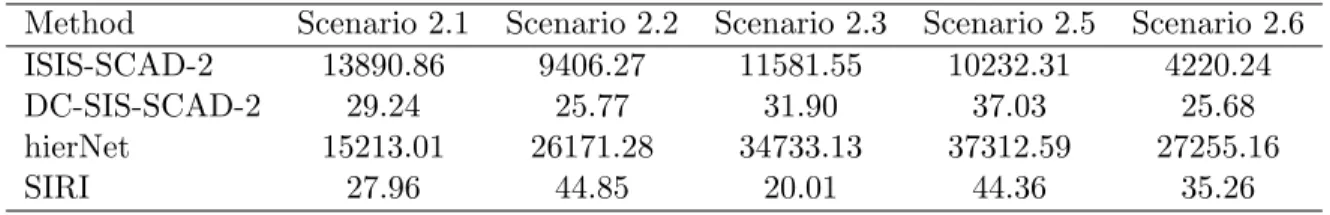
Table 2.6: Average running time (in seconds) of di↵erent variable selection methods under Scenarios 2.1-2.3, 2.5 and 2.6

Method Scenario 2.1 Scenario 2.2 Scenario 2.3 Scenario 2.5 Scenario 2.6 ISIS-SCAD-2 13890.86 9406.27 11581.55 10232.31 4220.24 DC-SIS-SCAD-2 29.24 25.77 31.90 37.03 25.68 hierNet 15213.01 26171.28 34733.13 37312.59 27255.16 SIRI 27.96 44.85 20.01 44.36 35.26

Simulations in Scenarios 2.1-2.4 were generated under the same model assumption as ISIS-SCAD-k and DC-SIS-SCAD-k, which gives them advantage in the comparisons. Under Scenarios 2.5 and 2.6 of Table 2.5, when the generative model goes beyond multiplicative interactions, we can see that SIRI-AE and SIRI-CE significantly outperformed other methods in detecting relevant predictors with low false positives.

(48)

2.4

Real Data Examples

We applied SIRI to two real data examples. The first example studies the problem of leukemia subtype classification with ultra-high dimensional features. In the second example, we treat gene expression level in embryonic stem cells as a continuous response variables, and are interested in selecting regulatory factors that interact with DNA and other factors to determine expression patterns of genes.

2.4.1

Leukemia Subtypes Classification

For the first example, we applied SIRI-CE to select features for the classification of a leukemia data set from high density A↵ymetrix oligonucleotide arrays (Golub et al., 1999) that have been previously analyzed by Tibshirani et al. (2002) using a nearest shrunken centroid method and by Fan and Lv (2008) using a SIS-SCAD based linear discrimination method (SIS-SCAD-LD). The data set consists of 7129 genes and 72 samples from two classes: ALL (acute lymphocytic leukemia) with 47 samples and AML (acute mylogenous leukemia) with 25 samples. The data set was divided into a training set of 38 samples (27 in class ALL and 11 in class AML) and a test set of 34 samples (20 in class ALL and 14 in class AML).

Table 2.7: Leukemia classification results

Method Training error Test error Number of genes

SIRI-CE 0/38 1/34 8

SIS-SCAD-LD 0/38 1/34 16

Nearest Shrunken Centroid 1/38 2/34 21

The classification results of SIRI-CE, SIS-SCAD-LD and nearest shrunken centroids method are shown in Table 2.7. The results of SIS-SCAD-LD and the nearest shrunken

(49)

centroids method were extracted from Fan and Lv (2008) and Tibshirani et al. (2002), re-spectively. SIRI-CE and SIS-SCAD-LD both made no training error and one test error, whereas the nearest shrunken centroids method made one training error and two test errors. Comparing with SIS-SCAD-LD, SIRI used a smaller number of genes (8 genes) to achieve the same classification accuracy.

2.4.2

Identifying Regulating Factors in Embryonic Stem Cells

The mouse embryonic stem cells (ESCs) data set has previously been analyzed by Zhong et al. (2012) to identify important transcription factors (TFs) for regulating the expression of genes. The response variable, expression levels of 12408 genes, was quantified using RNA-seq technology in mouse ESCs (Cloonan et al., 2008). To understand the ESC development, it is important to identify key regulating TFs, whose binding profiles on cis-regulatory regions are associated with corresponding gene expression levels. To extract features that are associated with potential gene regulating TFs, Chen et al. (2008a) performed ChIP-seq experiments on 12 TFs that are known to play di↵erent