A Thesis by WON JU LEE
Submitted to the Office of Graduate Studies of Texas A&M University
in partial fulfillment of the requirements for the degree of MASTER OF SCIENCE
August 2006
A Thesis by WON JU LEE
Submitted to the Office of Graduate Studies of Texas A&M University
in partial fulfillment of the requirements for the degree of MASTER OF SCIENCE
Approved by:
Chair of Committee, Lewis Ntaimo Committee Members, Sergiy Butenko
Jianbang Gan Head of Department, Brett A. Peters
August 2006
ABSTRACT
A Stochastic Mixed Integer Programming Approach to Wildfire Management Systems. (August 2006)
Won Ju Lee, B.E, Soongsil University Chair of Advisory Committee: Dr. Lewis Ntaimo
Wildfires have become more destructive and are seriously threatening societies and our ecosystems throughout the world. Once a wildfire escapes from its initial suppression attack, it can easily develop into a destructive huge fire that can result in significant loss of lives and resources. Some human-caused wildfires may be prevented; however, most nature-caused wildfires cannot. Consequently, wildfire suppression and contain-ment becomes fundacontain-mentally important; but suppressing and containing wildfires is costly.
Since the budget and resources for wildfire management are constrained in real-ity, it is imperative to make important decisions such that the total cost and damage associated with the wildfire is minimized while wildfire containment effectiveness is maximized. To achieve this objective, wildfire attack-bases should be optimally lo-cated such that any wildfire is suppressed within the effective attack range from some bases. In addition, the optimal fire-fighting resources should be deployed to the wildfire location such that it is efficiently suppressed from an economic perspective.
The two main uncertain/stochastic factors in wildfire management problems are fire occurrence frequency and fire growth characteristics. In this thesis two models for wildfire management planning are proposed. The first model is a strategic model for the optimal location of wildfire-attack bases under uncertainty in fire occurrence. The second model is a tactical model for the optimal deployment of fire-fighting
resources under uncertainty in fire growth. A stochastic mixed-integer programming approach is proposed in order to take into account the uncertainty in the problem data and to allow for robust wildfire management decisions under uncertainty. For computational results, the tactical decision model is numerically experimented by two different approaches to provide the more efficient method for solving the model.
ACKNOWLEDGMENTS
First and foremost I would like to express the deepest appreciation to my advisor, Professor Lewis Ntaimo. He is the one who always inspired me to finish this research from its inception and encouraged me to focus on the research. Without his vision, guidance, support, and consideration, this research would have not been possible. I have learned many things from him, and now I feel that I am a better researcher than ever. I would also like to thank my committee members, Professor Sergiy Butenko and Professor Jianbang Gan for their consideration and encouragement. They were eager to help me whenever I needed their help and advice.
I thank my friend, Byungsoo Na. He always helped and encouraged me whenever I went through hard time during my master’s degree. I also would like to thank my officemates, Eric Beier and Matthew Tanner for the valuable comments and knowl-edge on stochastic programming. I also would like to acknowlknowl-edge my friends and colleagues at the Department of Industrial & Systems Engineering, Texas A&M uni-versity who cheered me up all the time.
Finally, I am greatly thankful to my lovely wife, Young Lan. She always has been with me whenever I am happy or I get through hard time. Her love, sacrifice, and prayers made this research possible. I will always remember her love forever. Also I always remember my families who pray for me back home in my country.
TABLE OF CONTENTS CHAPTER Page I INTRODUCTION. . . . 1 II LITERATURE REVIEW . . . . 4 A. Preliminaries . . . 4 B. Strategic Decision . . . 9 C. Tactical Decision . . . 12 D. Stochastic Programming . . . 15
III ATTACK-BASE LOCATION AND RESOURCE ALLOCA-TION MODEL . . . . 19
A. Problem Description . . . 19
B. Proposed Model Formulation . . . 21
1. Parameters . . . 21
2. Decision Variables . . . 22
C. Model Description . . . 23
IV RESOURCE ALLOCATION MODEL FOR WILDFIRE CON-TAINMENT . . . . 28
A. Problem Description . . . 28
B. Proposed Model Formulation . . . 29
1. Parameters . . . 29
2. Decision Variables . . . 30
C. Model Description . . . 31
V SOLUTION APPROACH . . . . 33
A. L2 with Benders’ Cuts Algorithm . . . . 33
B. Impementation . . . 39
VI COMPUTATIONAL EXPERIMENTS . . . . 42
A. Wildfire Containment Decisions for a Small-Scale Fire . . . 42
1. Basic Data . . . 42
2. Analysis of Solution of the Instance wfcp 7 6 5 . . . . 44
CHAPTER Page
4. Findings and Conclusions on wfcp Instances . . . 53
B. Wildfire Containment Decisions for a Large-Scale Fire . . . 54
1. Generation of Scenarios and Experimental Design . . . 54
2. Computational Results of wfcpu Instances . . . 55
3. Findings and Conclusions of wfcpu Instances . . . 59
C. Overall Findings and Conclusions . . . 59
VII CONCLUSIONS AND FUTURE WORK . . . . 64
A. Conclusions . . . 64
B. Contributions of This Research . . . 65
C. Future Work . . . 66 REFERENCES . . . . 67 APPENDIX A . . . . 71 APPENDIX B . . . . 76 APPENDIX C . . . . 85 APPENDIX D . . . . 94 APPENDIX E . . . . 100 VITA . . . . 111
LIST OF TABLES
TABLE Page
I Total fires and acres . . . . 1
II Total suppression cost . . . . 2
III Scenario data generation for wfcp instance . . . . 43
IV Fire-fighting resource characteristics . . . . 44
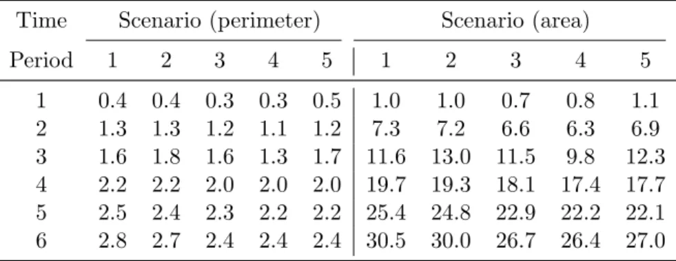
V Fire perimeter and burned area for 5 scenarios. . . . 44
VI Result of wfcp 7 6 5 . . . . 45
VII Results of 5 instances under perfect information . . . . 45
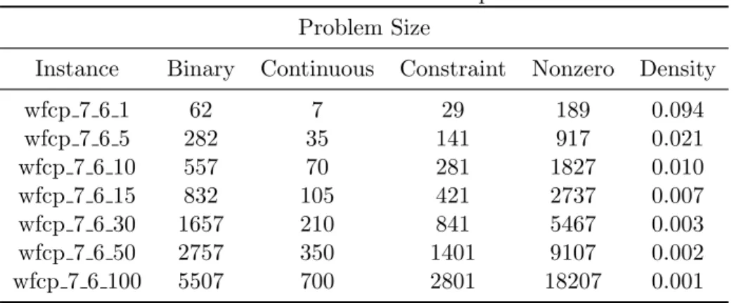
VIII Problem size of wfcp instances . . . . 47
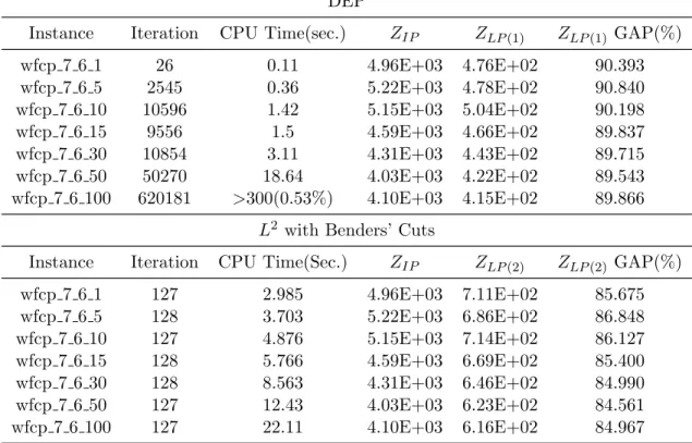
IX Results of wfcp instances with unconstrained budget . . . . 48
X Optimal resource mix of wfcp instances with unconstrained budget . 49 XI Results of wfcp instances with constrained budget . . . . 51
XII Results of wfcp instances with NVC per hectare $20 . . . . 52
XIII Results of wfcp instances with NVC per hectare $1000 . . . . 53
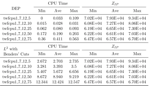
XIV Summary of twfcpu1 instances with unconstrained budget . . . . 57
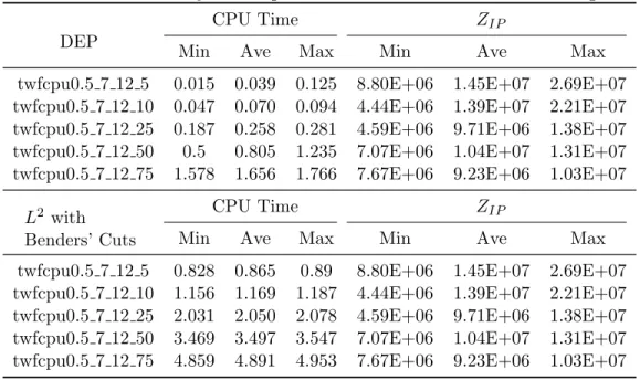
XV Summary of twfcpu0.5 instances with constrained budget. . . . 58
XVI Optimal resource mix of wfcp instances with constrained budget . . . 71
XVII Optimal resource mix of wfcp instances with NVC per hectare $20 . 71 XVIII Optimal resource mix of wfcp instances with NVC per hectare $1000 72 XIX Summary of twfcpu1 instances with NVC per hectare $20 . . . . 72
TABLE Page
XX Summary of twfcpu1 instances with NVC per hectare $1000 . . . . . 73
XXI Summary of qwfcpu1 instances with unconstrained budget . . . . 73
XXII Summary of qwfcpu0.5 instances with constrained budget . . . . 74
XXIII Summary of dwfcpu1 instances with unconstrained budget . . . . 74
XXIV Summary of dwfcpu0.5 instances with constrained budget . . . . 75
XXV Unconstrained budget (tripling resource production rate) . . . . 77
XXVI Constrained budget (tripling resource production rate) . . . . 78
XXVII Fixed NVC $20 (tripling resource production rate) . . . . 79
XXVIII Fixed NVC $1000 (tripling resource production rate) . . . . 80
XXIX Unconstrained budget (quadrupling resource production rate) . . . . 81
XXX Constrained budget (quadrupling resource production rate) . . . . . 82
XXXI Unconstrained budget (doubling 14 resources production rate) . . . . 83
XXXII Constrained budget (doubling 14 resources production rate) . . . . . 84
XXXIII Unconstrained budget (tripling resource production rate) . . . . 86
XXXIV Constrained budget (tripling resource production rate) . . . . 87
XXXV Fixed NVC $20 (tripling resource production rate) . . . . 88
XXXVI Fixed NVC $1000 (tripling resource production rate) . . . . 89
XXXVII Unconstrained budget (quadrupling resource production rate) . . . . 90
XXXVIIIConstrained budget (quadrupling resource production rate) . . . . . 91
XXXIX Unconstrained budget (doubling 14 resources production rate) . . . . 92
XL Constrained budget (doubling 14 resources production rate) . . . . . 93
TABLE Page XLII wfcpu 100 scenarios . . . . 100
LIST OF FIGURES
FIGURE Page
1 Cost + NVC[9] . . . . 8
2 Convergence of wfcp 7 6 5 . . . . 50
3 FARSITE Wildfire Simulator . . . . 54
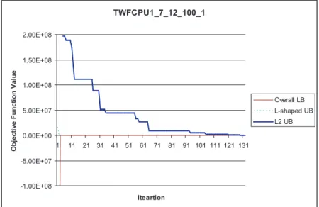
4 Convergence of twfcpu1 7 12 100 . . . . 56
5 Budget vs. Objective Function Value . . . . 60
6 NVC vs. Objective Function Value . . . . 61
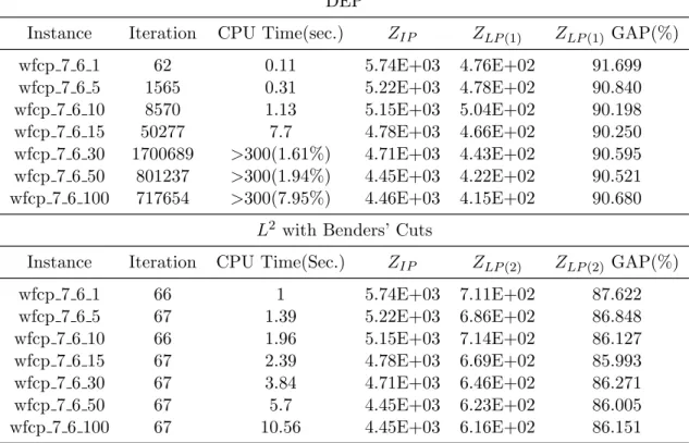
7 DEP vs. L2 with Benders’ Cuts (Small-Scale Fire) . . . . 62
CHAPTER I
INTRODUCTION
Damage caused by wildfires has been a serious problem to our society. In 2005 more than 66,000 wildfires were reported and more than 8 million acres were burned in the US alone (see Table I). Also in each year, a huge budget is allocated for wildfire suppression and containment (see Table II) [1]. It is also estimated that more than 11,000 communities adjacent to federal lands are at risk from wildfires [2].
Table I. Total fires and acres
Year Fires Acres Year Fires Acres 2005 66,552 8,686,753 1999 93,702 5,661,976 2004 77,534 6,790,692 1998 81,043 2,329,709 2003 85,943 4,918,088 1997 89,517 3,672,616 2002 88,458 6,937,584 1996 115,025 6,701,390 2001 84,079 3,555,138 1995 130,019 2,315,730 2000 122,827 8,422,237 1994 114,049 4,724,014
It is imperative to control these catastrophic wildfires in very efficient ways be-cause the budget and the resources are limited. One possible way to deal with this problem is to invest on the prevention effort. Prevention effort may include education, campaign, or patrol. Some human-caused wildfires may be prevented through this prevention effort. However, nature-caused wildfires cannot be prevented. Thus, it is necessary to contain the fires while they are small to minimize the associated costs and damage. Failure to contain a small fire may result in an escaped destructive huge fire. To contain the fires while they are small, it is important to deploy the fire-fighting resources in efficient ways. Consequently, it becomes very important to
consider the strategic and tactical decisions in wildfire management.
Table II. Total suppression cost Year Total Suppression Cost 2004 $890,233,000 2003 $1,326,138,000 2002 $1,661,314,000 2001 $917,800,000 2000 $1,362,367,000 1999 $523,468,000
In terms of the strategic decisions, the location of the wildfire attack-bases and the allocation of the fire-fighting resources should be strategically taken into account. In terms of the tactical decision, an optimal mix of the fire-fighting resources must be determined. These strategic and tactical decisions may help to reduce the chance that the wildfire becomes a destructive huge fire. Mathematical programming such as LP may be useful to model these decisions. However, LP does not take into account the randomness or uncertainty in the problem data since fire behavior is stochastic. Thus stochastic programming approaches are needed in order to take into account the stochastic factors of the problems.
This thesis is organized as follows. In chapter II, wildfire related literatures is reviewed, and the basic concepts of the stochastic programming are introduced. In chapter III, a new stochastic mixed inter programming model for the attack-base lo-cation and resource allolo-cation is presented. A new stochastic mixed integer program-ming resource allocation model for wildfire containment is presented in chapter IV. Chapter V provides solution methods for solving the proposed models. Computa-tional results of the model proposed in chapter V are given in chapter VI. Finally,
CHAPTER II
LITERATURE REVIEW
Wildfires have become more destructive and are seriously threatening our ecosystems and societies all over the world. It is therefore imperative to make great efforts to reduce the devastation wildfire damage by setting up effective wildfire management plans. The scope of the wildfire management is broad. It includes wildfire contain-ment and suppression. To utilize the limited budget and resources more efficiently, it is important to make optimal strategic decisions and tactical decisions. The strategic decisions include long-term planning for airtanker base location and resource allo-cation. The tactical decisions include short-term planning and scheduling for the resources with respect to actual wildfire occurrence. Mathematical programming and simulation methods are widely used in making these strategic and tactical decisions. This chapter is composed of four sections. Section A provides preliminary knowledge related to wildfire management systems. Section B provides strategic decision models of wildfire management. Section C provides tactical decision models of wildfire man-agement, and finally section D provides a brief review of the stochastic programming ideas that will be employed to solve the proposed model later chapter.
A. Preliminaries
In terms of wildfire management, analyzing wildfire economics or estimating the prob-ability of wildfire occurrence are important topics that give fundamental background to investigate wildfire-related problems. More fundamentally, it is also important to know how the wildfire management systems have evolved and what is needed to make the systems more effective.
to reduce the damage to the natural resource and risk to human. [3] researched on fire risk in the wildland-urban interface (WUI). WUI is the area where houses and dense vegetation exist together. It is known that WUI covers 10% of the United States [3]. The objective of the study in [3] was to identify the risk of severe wildfire in WUI areas, and how many people and houses were statistically affected through the case of northern lower Michigan. The researchers quantified fire risk by empirical methods of fire occurrence. The results may be useful in determining the location of emergency service site or fire-fighting resource sites.
[4] conducted research on the economic analysis of the relationship between value of resource protected and suppression expenditure of wildfires. This study may play a key role in determining the economic efficiency of suppression and containment activities. [4] argue that the benefit of suppression efforts should be greater than cost of resource value changes that would have burned with no suppression effort. The authors conclude that the expenditure on suppression is worthwhile if benefit is greater than cost.
There has been much effort to evaluate and quantify wildfire risk. The National Fire Danger Rating System is the one example of this effort [5]. It is provided the methods of quantifying wildfire risk [5]. One of the significant outputs includes the fire danger map based on fire weather variables such as temperature, humidity, wind and danger variables such as burning index, fire potential index, spread component. Based on these variables, three different fire risk probabilities can be defined: (1) The probability of fire occurring, defined as the probability of a fire of size greater than 0.04ha (hectare) occurring at a given location in a given day, (2) the conditional probability of a large fire given ignition, where large fire is defined as size of more than 40ha, (3) the unconditional probability of a large fire that is defined as the product of (1) the probability of fire occurring and (2) the conditional probability of a large fire
given ignition. Decisions on fire containment and suppression resource deployment may be made based on this (3) unconditional probability. These probabilities can be used to get the expected number of fires in a given region for a given time period. If a given area is divided into grids, each grid can be assigned its own probability of fire occurrence, and binary random variable (1 if fire occurs, 0 otherwise). Then the distribution of the total number of fires over entire areas is the Poisson-Binomial distribution. Thus sum of the probabilities of each grid gives the expected number of fires. Also the Poisson distribution can be employed to obtain confidence intervals.
Economists have expanded the methods of evaluating and quantifying the total economic value of wildland. Some methods of evaluating the economic value of wild-land has been suggested by [6]. Wildwild-land ecosystems can be viewed as natural capital that can produce a wide range of goods and services for mankind. Generally, timber, easily exchanged and quantified in terms of price, is considered as the most valuable goods from wildland. However there are many other outputs from wildland such as carbon storage, minerals, soil productivity, recreational use, etc. Some of them are not easily quantified as economic value. When dealing with wildfire, assessing the value of the wildland to be protected is extremely important since the solution for many kinds of wildfire suppression and containment problems depend on the eco-nomic value of the area. In this thesis, the ecoeco-nomic value of the area is referred as value-at-risk.
Since damage caused by wildfire is composed of tangible and intangible factors, it is extremely difficult to quantify the economic value of the damages. [7] quantified the economic value of the damages caused by wildfires in Florida. They investigated seven major categories of damages, that is, pre-suppression costs, suppression costs, disaster relief expenditures, timber losses, property damage, tourism-related losses, and human health effects. This research is worthwhile because it quantifies economic
impacts of wildfires systematically and empirically.
[8] proposed the theoretical framework of wildfire economics, that is the Cost plus Net Value Change (C+NVC) model. This model has been used as a principal model of evaluating wildfire economics. This model minimizes the cost of wildfire by minimizing sum of the pre-suppression cost, suppression cost, and net value change. The pre-suppression cost is the fixed cost that is spent before the fire season starts to minimize overall wildfire occurrences through education, patrol, campaign, or in-vestment on resources or new facilities. The suppression cost is the cost that is spent during the fire season. Most of the cost is associated with fire suppression and con-tainment operation cost. The NVC is the cost that is incurred by the damage from wildfire during the fire season. The C+NVC has become the most widely used eco-nomic theory in the text of wildfire management.
The C+NVC model was reformulated by [9] by correcting some of the assump-tions. The original model treats suppression cost as a output while the corrected model treats suppression cost as a input. Also the original model assumes that suppression and pre-suppression costs are negatively correlated while the corrected model assumes that only suppression cost varies. As a result, the corrected C+NVC model provides the global minimum of the function. Figure 1 provides the corrected (C+NVC) framework. It is shown that the pre-suppression cost is fixed since it is spent before the fire season begins. Also, it can be inferred that suppression cost and Net Value Change are negatively correlated since the more suppression efforts we have, there tends to be less burned area by wildfires. The sum of the suppression cost, the pre-suppression cost, and the net value change provides the global function of the C+NVC. Since it forms a convexity, global minimum can be found by minimizing this function.
Fig. 1. Cost + NVC[9]
Before examining detailed literature on containment and suppression, it is worth-while to review broad research on wildfire management. [10] provided good review of operational research studies in forest fire management by taking into account several topics such as prevention and fuel management, strategic and tactical detection plan-ning, operations research techniques on fire suppression, and fire impact management policy model. In terms of operations research methods on fire suppression, they are subdivided into four topics. (1) Resource acquisition and strategic deployment in-volve determining what resources to acquire and where to locate them. (2) Resource mobilization involves resource re-allocation due to fluctuating fire load. (3) Initial attack dispatching deals with resources that are dispatched to the fire location in the early stages of the fire occurrence. Initial attack dispatching may be complicated since the precise fire location, size and many other fire related variables are uncertain. (4) Extended attack management involves suppression and containment effort to the
fire that is escaped from initial attack and developed into a large fire.
B. Strategic Decision
Strategic decisions of wildfire management systems are the long-term plans that should be carefully considered because it may require much time and financial in-vestment resources and may not be easily modified once it is executed. Some of the strategic decision models are conceptual, while others are more concrete. And many of the strategic models are related with the attack-base location problems. [11] pro-vides a good review of the location problems. Some of the problems are defined as follows. Location set covering problem (LSCP) is to locate the least number of facili-ties that are required to cover all demand points. Maximal covering location problem (MCLP) is to seek the maximal coverage with a given number of facilities and does not necessarily require to cover all demand points. The objective of P-median prob-lem is to optimize the average (total) distance between the demand points and the facilities, and the objective of P-center problem is to minimize the maximum distance between the demand points and the facilities.
A new fire management paradigm that takes into account broad objectives has been proposed by [12]. The authors focus on a performance-based system. Most of the previous models optimize the suppression-related problems. Instead, the proposed system is conceptual and it is composed of such elements as fire and land management plans, ecosystem and fire simulators, fire management resources, program constraints, fire response, fuels treatment, and performance evaluator. [12] recommends that the geographic information should be carefully taken into account in making the fire man-agement plans.
in [13]. The model decides where to locate wildfire attack-bases among potential base locations. A given area is divided into a set of sub-areas in the model. The value-at-risk concept is used to quantify the value of the sub-area and to prioritize the sub-area in terms of the economic value. Also the authors take the distance from base to sub-area (demand point) into consideration in the objective function of the model since fire scale, or fire perimeter gets bigger with time. The model utilizes the historical fire data of the fire occurrence location and considers several different time periods. The model is then optimized with respect to the different time peri-ods. Consequently, the solutions from the model may not be appropriate in making strategic decisions since each time period considered may provide different solutions of the base location.
Several different location models in locating wildfire attack-bases were analyzed in [14]. These models include covering, p-mediam, p-center, and some hybrid models. These models give various solutions that make sensitivity analysis possible. These models also utilize the historical fire occurrence data of the several different time peri-ods as [13] did. Consequently, the solutions from the models may not be appropriate in making strategic decisions.
An optimization model that minimizes the wildfire damage by locating and de-ploying fire-fighting resources in critical locations was proposed in [15]. The proposed model mainly has two parts: a geographic information system (GIS) module and a mathematical programming module. Based on the GIS information, the demand area to be covered is subdivided into a number of non-uniform, and non-overlapping sub-areas. The data collected by GIS are used as input to an mathematical programming module. By taking into account the data from the GIS module, the mathematical programming module determines the optimal fire-fighting resource locations. Maxi-mal covering location model was employed in the mathematical programming module.
As an extension of [15], an integrated framework for wildfire control is proposed in [16]. It has three major modules; a mathematical module, a simulation module and a GIS module. The mathematical module provides strategic decision solutions for long-term plans that include how many resources to need to cover the given area, and where to locate resources. The simulation module provides tactical solutions for short-term decision making. In the mathematical module, they utilize the set cover-ing problem and the maximal covercover-ing location problem. In the set covercover-ing problem, it assumes that one vehicle assigned to each demand point can suppress all the wild-fires within its coverage. The simulation module considers the resource re-allocation based on updated fire figures, thus it may not be appropriate to explain the detailed deployment plan of the optimal mix of resources for a specific fire.
A model that specifies where to locate the service site and how many resources such as emergency vehicles to be assigned at each site is provided in [17]. This emergency medical service application has much similarity to wildfire management application since the emergency location can be viewed as the wildfire location and the service site can be viewed as the site where wildfire attack resources are based. One of the significant characteristics of this model is that it takes into account the un-certainty of the demand of emergency service by employing stochastic programming approaches. Without the stochastic factors in this model, it belongs to the general class of the covering problem. It employs a probabilistic constraint approach that allows demand requests to be satisfied with a certain reliability α.
More advanced location problems through the evolution of ambulance locations and relocation models are reviewed in [18]. As previously mentioned, emergency med-ical service application has much similarity to wildfire management application. This paper reviews probabilistic models rather than the deterministic location models. Maximum expected covering location problem (MEXLP) and maximum availability
location problem (MALP) are the probabilistic versions of the maximal covering loca-tion problem. MEXCLP maximizes the expected coverage of all demand areas. It is assumed that servers operate independently and that all servers have the same busy probability. MALP maximizes the demand that should be covered with a given reli-ability α. Largely MALP may be sub-divided into 2 categories; MALP I and MALP II. MALP I uses the same busy fraction for all potential location sites while MALP II relaxes the assumption that the busy fraction is identical for all sites.
C. Tactical Decision
Tactical decisions in wildfire management deal with relatively short-term decisions. These include the mix of the resources to contain a particular fire, scheduling of airtanker based on fire demands, or fire behavior simulation. The goal of these ap-proaches is to analyze the short-term wildfire related problems and provide optimal decisions in order to minimize the damage or risk of wildfires by containing wildfires in efficient ways.
A tactical decision model that determines the optimal mix of the fire suppression resources for the particular fire to minimize the C+NVC function is proposed by [19]. This model fits well when it needs to be answered which resources to deploy and when to contain the fire with minimum cost. However, this model assumes that fire perimeter in the particular time period is deterministic. That assumption may not be applicable in reality since fire growth behavior is stochastic.
A simulation approach for the wildfire containment is provided in [20]. Most of the simulation approaches are focused on estimating a fire’s capacity to spread. Instead, this model focuses on the interaction between the production of containment line and a fire’s capacity to spread. It allowed a flexible choices of the fire shape, and
different types of attack method by the resources. However, it may not be able to provide the optimal mix of the resources to minimize total cost within the budget and resource constraints. Rather it focuses on when to contain the fire with all available resources. By the nature of simulation, it may not be easy to find the optimal mix of resources with a small number of experiments since this simulation model only gives results with a set of given parameters in each run.
A mathematical programming model considering the daily basing rule of air-tankers is proposed in [21]. After a fire load profile is obtained, it assigns airair-tankers in each base and the airtankers move among the bases based on the fire load. The fire load varies from period to period, and basing airtankers is dependent on the fire load data that are prepared from the long-term historic data. The objective of the model is to minimize the incurred cost of basing airtakers. Thus one airtanker is not fixed in one specific air base. One of the strengths of this model is that it actually deals with daily use of airtankers based on demand. However it does not take into account such considerations as the fire which continues more than one day, rather it assumes that all demands are satisfied in one day by the airtanker.
A model that investigates how airtanker system performance is associated with initial attack range is proposed in [22]. This model uses a simulation method to in-corporate the complex systems that contain many stochastic factors. Systems that are composed of fire events and airtanker that serves fire are described as queueing systems just as they are customers and servers in the general queueing systems. It is defined that the fire arrival process as the non-stationary process since the daily fire load varies during the day. It is found that the initial attack range varies as a function of the daily fire load. As a result, they suggest that it is required to set initial attack range of individual airtanker to increase the efficiency of the suppression effort and minimize the associated cost.
A model that evaluates the performance of the initial attack of the airtankers is provided in [23]. When the probability of the fire occurrence within the initial attack zone of an airtanker base is specified, this model provides important informa-tion regarding expected flight distance between the airtanker base and a random fire location, and computes flight distance distribution. This is done by the mathematical procedure that uses data such as the coordinates of the base location, the geologi-cal distribution of fire occurrence. The model also takes the fire-start location, the distance between air-base and fire-start location as random variables. The results of the model are used to evaluate the performance of the airtankers, one of the most expensive resources in a wildfire fight.
Simulation models that simulates the wildfire spread and suppression are devised by [24], and [25]. Especially [24] employs the a discrete event system specification cell space approach. Its advantages are that it only considers active cells in computation and transmission of messages, thus it improves the efficiency of the simulation. In ad-dition, the cells in the simulation can be dynamically created and deleted as needed. The model considers static cells that stores geographic information and dynamic cells that may have different stochastic characteristics of weather conditions. These cells decide fire spread and fire-line intensity that play key roles in the simulation. From the simulation, the cells change the status; unburned, burning, and burned. And the status tells how fast and where the fire spreads. It also includes the suppression function so that the suppressant keeps the fire in the cells from propagating further. The National Fire Management Analysis System (NFMAS), especially the sensi-tivity analysis of the Initial Attack Analysis (IAA) processor is analyzed in [26]. The IAA is the fire simulator that simulates fire behavior and containment. The authors experimented the simulator with respect to different input parameters such as the fire spread rate, the production rate of suppression, the initial attack time, the fire
size at detection. It is found that the fire spread rate has the most impact on the results, and the fire size has least impact to the results. Also it is found that the economic analysis of wildfire on the IAA based on the C+NVC heavily relies on the escaped fires because they are composed of much portion in NVC, and the users of the IAA processor are required to determine whether the fires are the escaped fires or not. It is suggested that this action needs to be improved since this may lead to wrong estimation of C+NVC value.
D. Stochastic Programming
From the literatures of the strategic and the tactical decisions of wildfire management problems, it is found that there is much randomness or uncertainty in wildfire occur-rence and behavior. Therefore stochastic programming approaches are utilized to solve the proposed models that are introduced in later chapters. One of the most sig-nificant characteristics of the stochastic programming is that it can take into account uncertainty in the model. Good introductory reviews about stochastic programming can be found in [27], [28] and more details are provided in [29].
Since the uncertainty is inherited in fire behavior and occurrence, it is important to consider the randomness in modeling wildfire related problems. A stochastic mixed-integer programming (SMIP) deals with two generally difficult classes of problems: stochastic programs and integer programs. Therefore, by inheriting the properties of both generally difficult classes of problems, SMIP is regarded as the most chal-lenging classes of optimization problems. In general, a stochastic program evaluates the problem by optimizing it over possible future scenarios that represent alternative outcomes of the problem data. Two-stage recourse model is widely used in solving stochastic programs. In the two-stage setting, first-stage decisions are made without
full information on a random event. In the second-stage, after full information about the random event becomes available, the first-stage decisions are utilized and it takes recourse actions that may change the first-stage decisions. This procedure is repeated until the solution is converged. A general two-stage SMIP problem with recourse can be given as follows: SMIP1: Min c>x+E ˜ ω[f(x,ω,˜ )] (2.1) s.t.Ax ≤ b, (2.2) x ∈ X. (2.3)
where, c is the first-stage objective function coefficient, X is the first-stage decision feasible set (it may have integrality property), and Eω˜[.] is the mathematical expec-tation operator with respect to the random variable ˜ω. The function f(x, ω) denotes the second-stage recourse function under a realizationω of ˜ω. This evaluates the cost of recourse actions to guarantee the feasibility of the first-stage decisionsxunder this realization. The function f(x, ω) can be given as follows:
SMIP2: f(x, ω) = Min q(ω)>y(ω), (2.4) s.t.W(ω)y(ω)≤r(ω)−T(ω)x, (2.5)
y(ω) ∈ Y. (2.6)
where, Y is the second-stage decision feasible set (it may have integrality property), y(ω) is the second-stage decisions under a realization ω, and W(ω) and T(ω) are
matrices while r(ω) is a vector, all with appropriately dimensioned sizes. In the stochastic programming literatureW(ω) andT(ω) are referred to as the recourse and technology matrices, respectively. SMIP2 is referred to as a scenario subproblem. It is also generally assumed that for all (x, ω), SMIP2 is feasible. This assumption is referred to as relatively complete recourse. It is also assumed that there is a finite collection of scenarios ω denoted by Ω. If matrix W is independent of ω, problem (2.1-2.6) is said to havefixed recourse. Otherwise, the problem is said to haverandom
recourse.
When only continuous decision variables are embedded in the two-stage recourse model, L-shaped method [30] is the most widely used algorithm to the model. This method is based on the Bender’s decomposition method [31] where it is developed from the Kelley’s method [32]. Because of the linearity and convexity of theL-shaped method, it performs very efficiently in large-scale problems. However, it cannot be appropriate to solve the models that have integrality property in decision variables. When the integrality is introduced in the problem, some difficulties come with this property. This includes that the problem loses its convexity property, thus it may computationally takes long time to solve the problem, and may end up with failing to get to the optimal solution within the polynomial time. One way to overcome these difficulties is to introduce a tight valid cut similar to the cutting plane methods used in solving integer programming (IP). If all the variables in the first-stage are binary, and there are only continuous variables in the second-stage, the L-shaped method may still be used to solve this problem by implementing algorithms such that inte-grality holds in the first-stage. If both stages have integer variables, especially binary, we may be able to use Integer L-shaped method orL2 algorithm [29]. In this thesis, the L2 with Benders’ Cuts algorithm that takes the advantages of both L2 algorithm and L-shaped method is utilized and implemented to solve the proposed models. The
details of the algorithm are discussed in chapter V.
Equation (2.1-2.6) can also be written as one large-scale deterministic equivalent problem (DEP) in which all the scenarios are considered at once. The DEP can be given as follows: SMIP1: Min c>x+X ω∈Ω p(ω)q(ω)>y(ω), (2.7) s.t. Ax ≤ b, (2.8) T(ω)x+W(ω)y(ω)≤r(ω), ω∈Ω (2.9) x ∈ X, y(ω) ∈ Y. (2.10)
wherep(ω) is the probability that a random eventωoccurs. Since stochastic program-ming considers every possible scenarios in the problem, it will provide the valuable results which linear programming approach cannot provide. The DEP can be opti-mized by direct solvers such as CPLEX [33] since decomposition method is not ap-plied to the approach. However this DEP may not be efficiently utilized when solving large-scale problems. This issue is discussed in chapter VI through the computational experiments.
CHAPTER III
ATTACK-BASE LOCATION AND RESOURCE ALLOCATION MODEL In this chapter, a SMIP strategic decision model for airtanker attack-base location and resource allocation is proposed. The proposed model is extended from the de-terministic model in [17]. The key questions are where to locate the attack-bases and how many resources such as airtankers to be assigned to each base to minimize the total associated costs and value-at-risk of the given area. Since fire occurrence is stochastic, the randomness of the fire occurrence should be taken into account in the model.
A. Problem Description
In terms of the strategic decision model of the wildfire management systems, locating attack-bases and allocating fire-fighting resources to the attack-bases is one of the most important decisions that should be carefully considered in long-term planning. In reality, the fire-fighting budget is generally not enough. Thus, it is extremely important to take maximum advantage of the budget by optimally locating attack-bases and allocating resources to each base. If this is not robustly planned, the wildfire suppression plan may not be working effectively. Consequently this may increase the probability of the wildfires becoming escaped fires that are usually occurred owing to the failure of initial wildfire attack. To locate the attack-bases optimally, we need to thoroughly investigate the area to be protected. This model assumes that the a set of candidate locations for the attack-bases are given and the entire area to be protected is divided by a set of sub-areas. It is also assumed that the the economic value of each sub-area, that is, the value-at-risk, and the wildfire occurrence frequency in each sub-area per the unit time are given. The unit time may be defined as the average
time it takes a single fire-fighting resource to suppress a single wildfire.
The randomness is inherent in the wildfire occurrence frequency in the model. The proposed model defines a scenario as the number of fire occurrences during a specific time period. The overall year is divided into a set of several time periods, where each time period can be a month, a quarter or a fire season. This rationale comes from the fact that the wildfire occurrence in each sub-area varies in each time period. For example, it is expected that there will be more wildfires in the dry weather season than in the wet weather season. Similarly, one can expect more fires in a vacation season than in a non-vacation season. Thus, the number of the wildfire occurrences in each sub-area during the unit time differs in each scenario (each time period). The intuition of the model is that the location of the attack-bases and the allocation of the resources should be dependent on the number of wildfires in each area, and the fire-fighting resources should be ready to be deployed to each sub-area based on the fire frequency during the unit time. If each sub-sub-area is not covered by enough resources, the value-at-risk associated with the sub-area may be at risk. The objective function of the proposed model takes into account the fixed cost of locating attack-bases, the variable cost of deploying resources from the bases to the sub-areas (it also can be considered as operating cost of fire-fighting resources during the unit time), and the total value-at-risk in danger due to the failure in assigning the optimal number of resources to the sub-areas. It is worthwhile to note that the overall variable costs in the planning time horizon can be calculated by multiplying the variable cost during the unit time by the number of the unit times during the planning horizon (the planning horizon may be considered as one year in this thesis). Thus this enables the model to take into account long-term strategic planning by taking into account one-time fixed cost and overall variable cost during the planning horizon.
B. Proposed Model Formulation
In the two-stage SMIP with recourse model, it selects attack-base locations among potential attack-base locations in the first-stage, so that the fire-fighting resources can be assigned to the base location. In the second-stage, given the attack-base locations and a collection of fire occurrence scenarios Ω, the corrective (recourse) actions are made. If the required number of resources are not assigned to some sub-areas, the variable costs associated with the base location and the sub-areas are reduced, but the value-at-risk associated with the sub-areas is increased. The objective of the two-stage recourse model is to decide the optimal base location and resource allocation to minimize the total associated cost by taking into account the randomness in wildfire occurrence with respect to overall scenarios. Let idenote the index for sub-areai∈I and j denote the index for potential attack-base location j ∈ J, where I and J are finite sets of sub-areas and potential attack-base locations.
1. Parameters B1 : budget limit of locating attack-bases
B2 : total budget limit of fixed and variable costs fj : fixed cost of locating attack-base at j
M : some large constant
P rω : probability of scenario ω∈Ω occurring.
vω
i : value-at-risk of sub-area iunder scenario ω∈Ω
cω
ij : variable cost of operating one resource from attack-base j to sub-area i
hω
i : average number of wildfire occurrences during the unit time in sub-area i
under scenario ω ∈Ω
n : number of unit times in one year
dij : distance between sub-area i and attack-base j
dmax : maximum one time attack effective distance of fire-fighting resources
N(i) : set of potential base indices that can cover sub-area i where it can be defined as N(i) ={j|dij ≤dmax}
M(j) : set of sub area indices that can be covered by attack-basej where it can be defined as M(j) ={i|dij ≤dmax}
-Remarks
n can be estimated by dividing one year by unit time
P rω can be estimated by dividing the total number of wildfires in an area
dur-ing one year by the total number of the wildfires durdur-ing the time unit (period) associated with the scenario ω. Thus it may be thought as the weight of the scenario with respect to one year.
2. Decision Variables
xj : 1 if attack-base location j is opened, and 0 otherwise
yω
ij : integer variable that indicates the number of the resources that cover
sub-area i from attack-base j under scenario ω ∈Ω zω
i : 1 if sub-area i is not assigned by the required number of the resources that
is equivalent tohω
We can now formally state our two-stage SMIP model as follows: Min X j∈J fjxj+E[h(xj,ωe)] (3.1) s.t. X j∈J fjxj ≤B1 (3.2) xj ∈ {0,1}, ∀j ∈J (3.3)
where for each outcome ω∈Ω, h(xj, ω) = Min X i∈I X j∈J cω ijyωij + X i∈I vω izωi (3.4) s.t. X i∈I X j∈J n∗cω ijyωij ≤B2− X j∈J fjxj (3.5) X j∈N(i) yωij−hωi +Mziω ≥0, ∀i (3.6) X i∈M(j) yω ij ≤Mxj, ∀j (3.7) yω ij :general integer, ziω ∈ {0,1}, ∀i∈I, ∀j ∈J (3.8) C. Model Description
In the model the first-stage objective function (3.1) ensures that the sum of the cost to locate the attack-bases and the expected variable cost and value-at-risk caused by wildfire occurrence is minimized. Constraint (3.2) indicates that the sum of the cost to locate the attack-bases is within the budget B1. the constraint (3.3) enforces the binary restrictions on xj.
The second-stage objective function (3.4) ensures that for the given opened attack-base locations, the sum of the associated variable cost and the sum of the value-at-risk associated with the sub-areas are minimized for the fire occurrence sce-narioω ∈Ω. The variable cost is incurred by operating one fire-fighting resource from its base to a specific sub-area and the value-at-risk associated with the sub-area is
incurred if the minimum required number of resources which should be greater than or equal to hω
i are not provided to the associated sub-area. (3.5) requires the sum of
the locating attack-bases and the sum of the variable cost based on the operation of the resources with respect to wildfire occurrence is within the total budget limit B2. The constraint (3.6) decides whether the value-at-risk associated with each sub-area at risk or not. If it is at risk which is not a favorable case, the value-at-risk associated with the sub-area is taken into account in the second stage objective function. The constraint (3.7) indicates that if any of the resources is assigned to a specific base location, the base should be opened. The restriction (3.8) indicates that decision variables yω
ij is binary variable, zjω is general integer variable by the nature of the
problem.
The rationale behind (3.5) is that the budget for the attack-base location is made on long-term basis and the budget for the variable cost are made on yearly basis. Since variable costcω
ij represents one time operating cost from attack-basej to
sub-area i, to estimate the annual operating variable cost and budget, n should be multiplied to the total variable cost during the unit time. Then this gives the annual operating cost.
There are three possible cases in the constraint (3.6). Here, it is worthwhile to note that the minimum required number of fire-fighting resources in the sub-area is greater than or equal to hω
i. In a given fire occurrence scenario, each sub-area i is
covered by the some number of resources. In first case, the decision variable yω ij, the
number of the resources that can be available for the sub-area i is greater than the required number of the resources that is equal to hω
i, and the decision variableziω can
take on a value of either 0 or 1. In this case, the value-at-risk associated with the sub-area i is not at risk, and as an indication of this information, it is desirable that the decision variable zω
i term in the second-stage objective function. And the objective function forces zω i
takes on a value of 0. The second case, the decision variable yω
ij takes the same value
that is equal to the value hω
i, and the decision variable zωi can take on a value of
either 0 or 1. Similar to the first case, it is desirable that zω
i take on a value of 0, and
the same logic used in the first case is applied in the second case. Thus, zω
i takes on
a value of 0. The third case, the decision variable yω
ij take the value that is less than
hω
i, and the decision variable ziω only takes a value of 1. Since there are not enough
resources available for the sub-area i, the value-at-risk associated with the sub-area i is at risk. Thus this fact adds the value-at-risk in the objective function where its goal is to minimize the associated total cost.
The rationale of this constraint is that the third case is desirable to be avoided. However, due to the limited availability of the total number of resources forced by the budget limit, if it cannot be fully responsible for the overall area, this model recommends that the resources should be allocated to the sub-areas that have more economic value than other sub-areas.
Another important rationale of this constraint is that during the unit time as many number as hω
i is required to be responsible for the sub-area i. And the
fire-fighting resources dedicated to the specific sub-area during the unit time cannot be deployed to the other sub-area at the same time. Thus, this model takes into account the situation where there are simultaneous fires in the area.
There will be two possible cases in the constraint (3.7). The first case is if at least one of the resources is assigned to the location j, xj takes on a value of 1. The
second case is if there is no resource assigned to the location j,xj can take on a value
of either 0 or 1. If this cases occurs, the second-stage objective function forces xj to
take on a value of 0 to minimize the objective function value. This constraint is a ‘linking constraint’ since it links the first and the second stages.
The proposed strategic decision model for attack-base location and resource allo-cation is extensions of such existing models as [13], [15], [16], [17] in several directions since it takes into account (1) the randomness in wildfire occurrence in different sub-area in different time period, (2) simultaneous fires, (3) overall operating variable cost as well as fixed cost, (4) value-at-risk which is incurred when a specific sub-area is not protected, and (5) budget limit. Also (6) it provides the solution of how many resources to be assigned to each base as well as where to locate the attack-bases. The model in [13] and [14] does not explain (1), (2), (3), (5), and (6). The model in [15] and [16] does not explain (1), (2), (3), (4), and (5). The model in [17] does not take into account (4) and (5). [17] takes into account (1) and (3), but the rationales used in [17] are different from those used in the proposed model in that the average number of the resources required to each sub-area is fixed, whereas the proposed model can be random in the proposed model, and it does not take into account the potential consequences when the required number of the resources cannot be assigned to each sub-area, whereas the proposed model in this chapter take into account the factor by introduction the value-at-risk concept and the decision variable zω
i . Thus
incorporat-ing the factor (1) through (6) makes this model capture much more realism than the previously proposed models. It provides valuable solution when decision makers in wildfire management want to make more realistic and systematic decisions in mak-ing long-term wildfire management plan and executmak-ing the limited budget optimally instead of making these important decisions in rule-of-thumb ways.
The proposed model can be solved by the SMIP algorithm that is described in chapter V. In this thesis, the computational experiments on this model are not con-ducted due to the some difficulties in acquiring the original data used in reality and extracting some important data used in the model from original data. Indeed, it is extremely difficult and takes much time to extract the realistic data such as vω
However, the model in chapter IV will be computationally experimented by the SMIP algorithm.
CHAPTER IV
RESOURCE ALLOCATION MODEL FOR WILDFIRE CONTAINMENT In this chapter, a SMIP tactical decision model for resource allocation for wildfire containment is proposed. The proposed model is based on the deterministic model by [19]. The proposed model is also based on the C+NVC model for wildfire economics proposed [8]. The proposed model minimizes the cost of wildfire by minimizing sum of the pre-suppression cost, the suppression cost, and the net value change. The key questions are which resources to be deployed and when the wildfire to be contained by minimizing the C+NVC objective function. Since the fire growth behavior is stochastic, the randomness of the fire growth behavior should be taken into account in the model.
A. Problem Description
The proposed model provides the solution that identifies the optimal mix of the fire-fighting resources required for the wildfire containment. The basic principle of how wildfire containment works is described in [34]. If the total fire line production constructed by the fire-fighting resources is greater than the total fire perimeter, it may be concluded that the fire can be successfully contained. The proposed model adapted the basic concept of the containment. In the model, it is assumed that fire line production rate, arrival time to the fire and operating cost of the resources is
deterministic. However, the fire growth characteristics such as fire perimeter and
net value change are assumed to be stochastic. Another assumption is that when a fire is initially ignited, resources will be deployed to the fire time period 0. It is defined that an instance of the stochastic fire perimeter as one fire growth scenario and optimize the model over a finite collection set of the scenarios that are assumed
to come from some fire simulation such as FARSITE [25] or DEVS [24]. The model considers different time periods and different type of resources. Under the budget and the resource production rate restriction, it is required to identify the fire can be whether contained or not. If it turns out to be contained, it is also required to identify the optimal mix of resources with the minimum C+NVC achieved. Since the resources cannot be fractional, it should have integrality property with the continuous fire perimeter. Thus the model has mixed integer variables.
B. Proposed Model Formulation
In the two-stage SMIP with recourse model, it selects resources and deploy them to the fire in the first-stage. In the second-stage, given resources and a collection of fire growth scenarios Ω, the corrective (recourse) actions are made on actual fire containment. Let idenote the index for fire containment resource i∈I and j denote the index for time period j ∈ J, where I and J are finite sets of fire containment resources and time periods, respectively.
1. Parameters B1 : pre-suppression budget limit
B2 : pre-suppression and suppression budget limit Hj : time period counter that takes a value of j
M : some large constant
P rω : probability of scenario ω∈Ω occurring
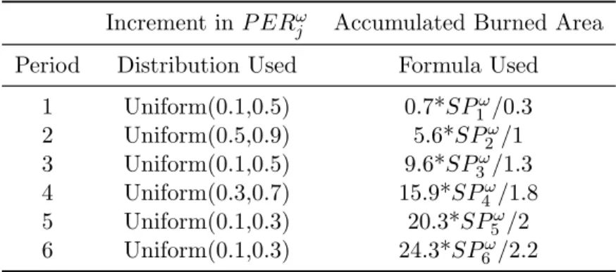
P ERω
NV Cω
j : increment in net value change for the period j under scenario ω ∈Ω
SPω
j : accumulated fire perimeter up to period j under scenario ω ∈Ω
Ci : hourly cost of operating resource i
Pi : rental cost of resource i
P Ri : line production rate of the resource i in kilometers (km)
Ai : arrival time to the fire of resource i
2. Decision Variables Zi : 1 if resource ihas been dispatched, 0 otherwise
Yω
j : 1 if fire is uncontained in periodj under scenario ω∈Ω , 0 otherwise
Dω
ij: 1 if containment achieved in period j using resourceiunder scenarioω ∈Ω
, 0 otherwise Lω
j : total line construction up to period j under scenario ω∈Ω
We can now formally state our two-stage SMIP model as follows:
Min X i∈I PiZi+E[h(Zi,ωe)] (4.1) s.t. X i∈I PiZi ≤B1 (4.2) Zi ∈ {0,1}, ∀i∈I (4.3)
where for each outcome ω∈Ω, h(Zi, ω) = Min X j∈J X i∈I CiHjDijω + X j∈J NV CjωYjω−1 (4.4) s.t. X i∈I X j∈J CiHjDijω ≤B2− X i∈I PiZi (4.5) X j∈J Lωj −X j∈J P ERωjYjω−1 ≥0 (4.6) X i∈I (Hj −Ai)P RiDijω −Lωj = 0, ∀j (4.7) SPjωYjω−1−Lωj −(M)Yjω ≤0, ∀j (4.8) X j∈J Dω ij ≤Zi, ∀i (4.9) Y0ω = 1 (4.10) Dω ij, Yjω ∈ {0,1}, Lωj ≥0, ∀i∈I, ∀j ∈J (4.11) C. Model Description
In the model the first-stage objective function (4.1) ensures that the sum of the pre-suppression and the expected suppression cost and net value change caused by burned area is minimized. The constraint (4.2) indicates that pre-suppression budget allowance is satisfied when resources are rented. Here the resource renting is consid-ered as the pre-suppression cost. The restriction (4.3) indicates that decision variable Zi will take on a value of 1 if resource i∈I is rented and 0 otherwise.
The second-stage objective function (4.4) ensures that for a given mix of fire-fighting resources determined in the first-stage, the sum of the associated suppression cost and net value change is minimized for the fire growth scenario ω ∈ Ω. The constraint (4.5) requires the pre-suppression budget and the suppression budget is satisfied when resources are deployed. The constraint (4.6) indicates that, in a given fire behavior scenario, the total fire line production constructed by the deployed
resource must exceed the total fire perimeter at some time period j ∈ J. If the dis-patched resources cannot contain the fire in given time periods, the problem turns out to be infeasible. The constraint (4.7) computes total fire line production based on the resources, deployed at time period 0. Thus, decision variable Lω
j represents
total fire line construction up to and including period j ∈ J. The constraint (4.8) provides information as to whether the fire is contained or not in the time period j ∈J. If the total fire line production constructed by the deployed resources in time period j is less than the total fire perimeter in the same time period, it is concluded that the fire is not contained yet. Then, as the indicator of the information, decision variable, Yω
j takes on a value of 1. Otherwise it takes on a value of either 0 or 1. If
contained, the second-stage objective function forces Yω
j to take on a value of 0 to
minimize the objective function value. This constraint is a ‘linking constraint’ since it links two different time periods. The constraint (4.9) ensures that in a given scenario if a particular resource i ∈ I is used during any of the time periods, Zi must take
on a value of 1 to take into account the associated pre-suppression cost. If not used, Zi may take a value of either 0 or 1. Then the same logic, used in the constraint
(4.8), forces Zi to take on a value of 0 to minimize objective function. The constraint
(4.10) simply makes the model start by initially igniting the fire in time period 0. The restriction (4.11) indicates that the decision variables Dω
ij, Yjω are binary variables,
and Lω
CHAPTER V
SOLUTION APPROACH
In chapter III and chapter IV, the strategic and the tactical decision model are pro-posed. These models have binary first-stage decision variables, and mixed integer variables in the second-stage. Thus, it falls in the class of the SMIP. Due to the difficult nature of SMIP, very few algorithms have been developed for this class of problems [29]. Moreover, the proposed models have random recourse property since the second-stage objective function coefficientqorW matrix in the second-stage con-straint set can have random elements. In this chapter, the solution method for the proposed models is introduced. Also, important issues in implementing the proposed algorithm are discussed.
A. L2 with Benders’ Cuts Algorithm
Both the proposed models fall in the SMIP with random recourse property. As a solution approach, both the L-shaped method and the L2 algorithm are efficiently applied. Laporte and Louveaux derive the L2 optimality cut for the piecewise linear approximation of the expected value function [29]. That L2 optimality cut requires lower bound of the recourse function. Thus, LP-relaxation of the proposed model is required to get the lower bound, and L-shaped method is utilized to get the lower bound value. Tighter lower bound value is essential to make the algorithm con-verged faster. Once the lower bound value is obtained by the L-shaped method, the L2 algorithm is utilized to solve the proposed models. To make the L2 algorithm converged faster in solving large-scale problems, the Benders’ cuts that are used in L-shaped method are applied in L2 algorithm. We call the proposed algorithm ’L2 with Benders’ Cuts Algorithm’. This approach provides a very tighter initial cut as
well as generates two strong valid inequalities that are the L2 optimality cut and the Benders cut in every iteration which significantly reduce the computational time in solving large-scale SMIPs. Before stating the algorithm, some preliminaries are introduced as follows.
• Original problem is given as below.
Min c>x + q>y (5.1)
s.t. Ax ≥ b (5.2)
T x +W y ≥ r (5.3)
x: binary, y : mixed integer (5.4)
q, W, r may have randomness, and let ωe denote random, and ω denote any realiza-tion of eω variable. Then it can be decomposed as below where first-stage only have deterministic data, and second-stage may have stochastic and deterministic data.
1st Stage: Min c>x + E e
ω[f(x,eω)] (5.5)
s.t. Ax ≥ b (5.6)
x: binary (5.7)
where for any realization ω ofωe we have
2nd Stage: f(x, ω) = Min q(ω)>y (5.8) s.t. W(ω) ≥ r(ω) − T(ω)x (5.9)
L-shaped Method
The L-shaped method is a efficient algorithm in solving two-stage recourse model if all the decision variables are continuous. Although the proposed models have mixed integer variables, the L-shaped method is utilized in solving the proposed models by applying LP-relaxation. This give the lower bound value Lthat is used in generating the L2 optimality cut in theL2 algorithm. Thus the followingL-shaped method pro-cedure is applied to get the lower boundL. For notational conveniences, it is assumed that there are only equality constraints.
Step[0] : Initialization
Let x0 be given.
Set ²≥0, LB=−∞, U B =∞, k ←0
Step[1] : Solve Subproblem
Let s be scenario index, then for s = 1,· · ·,S Solve fk
s = Min qs>y
s.t. Wsy = rs − Tsxk
y ≥0
If infeasible for some s: Generate feasibility cut -Get dual extreme ray: µk
s -Compute αk = µks > rs βk = µks > Ts -Go to Step[2]
Else if feasible ∀ s: Generate optimality cut - Get πk s - Computeαk = P spsπks > rs
βk = P
Spsπsk
>
TS whereps: probability of scenario s
Upper Bounding
Compute UB:
Vk = c>xk + P spSfsk
UB = min{Vk, UB}
If UB is updated, set incumbent solution to x∗ =xk
Go to Step[2]
Step[2] : Add Cut to Master Problem and Solve
If some subproblem was infeasible Addβ>
kx ≥ αk to master problem
Else
Addβ>
kx + η ≥ αk
Solve the master problem to get {xk+1, ηk+1} and Vk+1 as the master problem’s ob-jective value Lower Bounding LB = max{Vk+1, LB} Master Problem Vk+1 = Min c>+η s.t. Ax=b β> t x+η ≥αt, t∈θk β> t x ≥αt, t∈θk x≥0
Where θk denotes iteration index set at which an optimality cut is generated,
and θk denotes iteration index set at which a feasibility cut is generated
Step[3] : Termination If UB−LB ≤ ²|UB| Stop ELSE k←k+ 1 Return to Step[1]
L2 with Benders’ Cuts Algorithm
Once the lower boundLof the recourse function is obtained by theL-shaped method, the L2 with Benders’ Cuts algorithm is applied to solve the proposed models. The detailed steps of the algorithm are as follows.
Step[0] : Initialization
Let ² ≥ 0, x1 ∈ Ax≥b, x∈ {0,1}, be given. Also let L be obtained by L-shaped method.
Set v1← −∞, V1← ∞, k ←1
Step[1] : Solve subproblem for all ω∈Ω
Step[1-1] : Solve LP-relaxation of the subproblem:
Apply Step[1] in L-shaped method by applying LP-relaxation to solve subproblem. (Not to apply ’Upper Bounding’ part in Step[1])
Get the dual solutions of the subproblem, then create Benders cut.