An Overtaking Decision Algorithm for Networked Intelligent Vehicles Based on Cooperative Perception

(1)

An Overtaking Decision Algorithm for Networked Intelligent Vehicles

based on Cooperative Perception

Milos Vasic

Gael Lederrey

I˜naki Navarro

Alcherio Martinoli

Abstract— This paper presents an overtaking decision al-gorithm for networked intelligent vehicles. The alal-gorithm is based on a cooperative tracking and sensor fusion algorithm that we previously developed. The ego vehicle is equipped with lane keeping and lane changing capabilities, as well as a forward-looking lidar sensor. The lidar data are fed to the tracking module which detects other vehicles, such as the vehicle that is to be overtaken (leading) and the oncoming traffic. Based on the estimated distances to the leading and the oncoming vehicles and their speeds, a risk is calculated and a corresponding overtaking decision is made. We compare the performance of the overtaking algorithm between the case when the ego vehicle only relies on its lidar sensor, and the case in which it fuses object estimates received from the leading car which also has a forward-looking lidar. Systematic evaluations are performed in Webots, a calibrated high-fidelity simulator.

I. INTRODUCTION

Overtaking other vehicles accounts among the leading causes of motor vehicle accidents. They are known to have a high risk for a fatal outcome. In 2013, there was a total of 81000 accidents while overtaking in the USA [1]. These accidents can be, among other reasons, due to a wrong driver’s judgment or impaired visibility conditions.

It is well known that distances to remote objects and their relative velocities can be estimated more accurately using sensors than by bare eyes. Vehicles’ built-in intelligence can therefore be a useful aid to human drivers in these situations. However, there exist situations in which individual intelligent vehicles cannot perform very well: no matter what sensor technology is used, all sensors suffer from limited range, Field Of View (FOV), or non line-of-sight conditions to some extent. Hence, cooperation of vehicles by the means of exchanging the sensing data or track estimates can be advantageous.

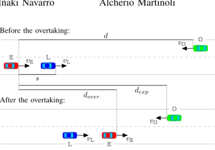
In this paper, we consider a sample scenario depicted in Fig. 1. It introduces three types of cars: the ego (_E), the leading (L) and the oncoming (O) cars. The car E is

an intelligent vehicle which contains sensors enabling it to perceive the environment and estimate its state. It processes the information and, once it encounters a slower car ahead, assesses the risk of overtaking and makes an overtaking decision. The carLis any car that finds itself driving in front

of the car E, on the same lane at lower speed. It may be

equipped with sensors and may share its information with the carEthrough communication. The carOis any car that drives

The authors are with the Distributed Intelligent Systems and Algorithms Laboratory, School of Architecture, Civil and Environmental Engineer-ing, École Polytechnique Fédérale de Lausanne (EPFL), Switzerland.

[email protected]

This work is financially supported by PSA Groupe and has benefited of the technical and administrative support of the EPFL’s Transportation Center.

Before the overtaking:

E _v E L vL O vO d s After the overtaking:

E v_E L v_L O vO dexp dover

Fig. 1. Example of an overtaking scenario.

on the passing lane of the car E, in the opposite direction.

It possesses no senors nor communication equipment, and it represents a potential hindrance to the overtaking maneuver.

In this paper we present an algorithm which assesses the overtaking risk and decides if the carE can overtake the car L safely. The algorithm relies on information provided by

a tracking and fusion algorithm previously presented in [2]. The carsEand Lrun the tracking algorithm, each using a

forward-looking lidar sensor. The car E additionally fuses

the information received from the car L, if available. We

consider two cases: the case in which the carLcooperates

with the car E by communicating its information, and the

case in which it does not.

The rest of the paper is organized as follows: Sec. II presents related work in the field. Sec. III summarizes the cooperative tracking and fusion algorithm, whereas Sec. IV presents the overtaking algorithm. Experimental evaluation is provided in Sec. V, while Sec. VI concludes the paper.

II. RELATEDWORK

Cooperative overtaking assistance systems are readily studied in the literature. In [3] a system which predicts when a potential lane-change is going to be performed by the driver of the ego-vehicle, cooperatively exchanges information with vehicles traveling in the opposite direction via the cellular network, and provides the driver with an estimate of the overtaking maneuver risk. It assumes that all oncoming vehicles are cooperative. Another assistance system is based on real-time video transmission [4]. This approach requires a high communication bandwidth. A cooperative overtaking assist system using an intelligent road surface is introduced in [5]. It requires investments in the infrastructure.

(2)

information obtained from on-board sensors, which is fed to the target tracking algorithm. The cooperative fusion algo-rithm is designed to minimize the communication bandwidth requirements (instead of raw data, tracks are communicated). One possible approach for multi-target tracking is a Probabil-ity Hypothesis DensProbabil-ity (PHD) filter, a generalization of the single-target Bayes filter. Its two well known implementations are based on a Gaussian Mixture (GM) model [6], and a Sequential Monte Carlo (SMC) model [7]. Works on fusing together the PHD intensities originating from different sources exist: an approach for GM-PHD intensities is given in [8] and for SMC-PHD intensities in [9]. Common for these works is the assumption that there exist a unique FOV (area) that is covered by all participating sensors simultaneously.

III. COOPERATIVEGAUSSIANMIXTUREPHD FILTER

To perform cooperative tracking of multiple targets (i.e., cars) using laser sensors, we use the Cooperative Gaussian Mixture PHD (C-GM-PHD) filter described in [2]. We summarize here the algorithm for completeness.

A. Multiple target tracking using a lidar sensor

The tracking algorithm works in two phases. The first phase pre-processes the laser point cloud with the aim to detect objects that resemble cars. First, the clustering of the point cloud is performed using the DBSCAN algorithm [10]. Then, lines and corners are fitted to clusters, and the one with smaller RMS error is preserved for each cluster. Finally, rectangles are fitted to lines and corners, and feature points are extracted. The set of object measurements is generated, where an object measurement is characterized using the center and orientation of a fitted rectangle,z= [x, y, θ]>.

The second phase represents the tracking algorithm based on the Gaussian Mixture Probability Hypothesis Density (GM-PHD) filter [6]. We model a target state using a vector

x= [x, y, θ, v, ω]>, wherexandyrepresent the center of the

tracked vehicle, θits orientation, and v andω its linear and rotational speed. Targets’ state hypotheses are called intensity and are modeled as a Gaussian Mixture. At timek−1 the intensity containing Jk−1 components with weights wk−1,

meansmk−1 and covariances Pk−1, where the weight of a

Gaussian component represents the number of targets that are represented using that component, has the form

Dk−1(x) = Jk−1

X

i=1

w_k(i₋)₁N(x;m_k(i₋)₁, P_k(i₋)₁) (1) The filter contains the predict and the update step, in which we use an Unscented Kalman Filter to deal with non-linearities. The motion model used in the predict step is the constant turn-rate and constant velocity model. To obtain the predicted intensity, the prior is multiplied by the proba-bility of survivalpS, which is a function of the hypothesis

state, and a birth intensityγk is added. It is given by

Dk|k−1(x) = Jk−1 X j=1 pS,k(m(_kj_|)_k₋₁)w(_kj−)1N(x;m (j) k|k−1, P (j) k|k−1)+ γk(x) (2)

κk(z), the probability of detectionpD,k(m (i)

k|k−1)dependent

on the mean of the Gaussian componenti(as a target can be occluded or leave the sensor FOV), the observation model

Hk and the observation noise covarianceRk. The first sum in

(3) represents missed targets, and the second updated targets. After the update step, the number of Gaussian components increases quadratically. Therefore, all Gaussian components with a very low weight are removed. Moreover, components that are close to each other are merged together and approxi-mated by a single component.

B. Cooperative fusion of PHD intensities

Vehicles located within the communication range of the carE can share their PHD intensities, i.e., their estimates

about targets in their FOV (in this work, this is only the car L). In the next paragraph, we explain how the car E

can fuse received PHD intensities with its own intensity, hence increasing its FOV beyond the one of its sensors, and decreasing uncertainty in the areas of overlapping FOVs.

Before fusion, we need to translate the received intensities (states and covariances of the target hypothesis) to the coordinate frame of the ego vehicle. This is done using the Approximate Transformation method [11], which adds uncertainties of frame poses to targets’ covariances. In order to avoid data incest problem, we use a General Covariance Intersection (GCI) algorithm, which offers a conservative way of fusing two Gaussian mixtures [12]. It is shown in [8] that GCI can be approximated to applying Covariance Intersection (CI) pairwise to components from the two intensities. To address the fact that the FOVs may not overlap entirely, we apply CI intersection only to components whose Mahalanobis distance from each other is less thanTF. We take the Gaussian

componentsiandj from intensitiesD1andD2respectively;

the fused component would have the following meanm(12)_ij , covarianceP_ij(12) and weight w_ij(12):

(3)

Free driving

Car following

Overtaking Abort overtaking

Leading car detected

Risk > Tabort

Behind the leading car Ahead the leading car Overtaking finished

Risk ≤ Tstart

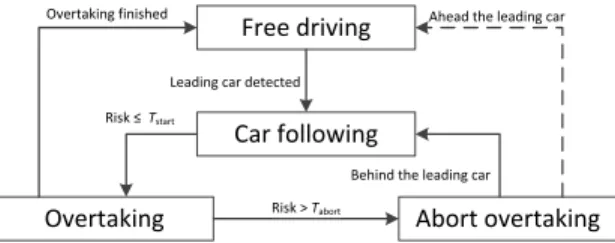
Fig. 2. A FSM defining the behavior of the ego car.

P_ij(12)=hW(P_i(1))−1+ (1−W)(P_j(2))−1i −1 (10) w(12)ij = wi(1) W w(2)j 1−W κ(W, Pi(1))κ(1−W, P (2) j ) · N m(1)_i −m(2)_j ; 0,P (1) i W + Pj(2) 1−W ! (11) where κ(W, P) = [det(2πPW −1 )]12 [det(2πP)]W2 (12) andW is the fusion weight whose value we set to0.5. We keep track of components that have been fused, and we copy the non-fused components to the result set (e.g., target that are in the FOV of only one vehicle).

IV. OVERTAKINGDECISIONALGORITHM

The behavior of the car_Efrom Fig. 1 is defined by a Finite State Machine (FSM) shown in Fig. 2. The car_Edrives freely on the road at its target speed until the tracking module detects a car driving on the same lane at a lower speed (leading car

L). The state of the carEis then changed tocar following,

where the adaptive cruise controller is engaged. As described in the remainder of this section, a risk for overtaking is continuously computed as a function of the presence and position of the car O, and the decision whether to start (or

eventually abort) the overtaking is based on a threshold.

A. State description

1) Free driving: the car E drives freely on the road at

target speedv0 while keeping centered in its lane.

2) Car following: The car_Efollows the car _L(which is driving on the same lane), maintaining a desired distance and time headway.

3) Overtaking: the car Ehas determined that it is safe to

overtake the car L(the risk that there is an oncoming car O

on that lane is low enough). It changes lane and performs overtaking at its desired speed v0.

4) Abort overtaking: the risk that the carOoccupies the

overtaking lane has become significant, thus the carEaborts

the overtaking maneuver.

B. Decision algorithm (FSM state transitions)

The initial FSM state is free driving. Once the car_L is detected, the state is changed tocar following.

In thecar following state, the overtaking risk is constantly computed. The risk is defined between 0 and 1, and it depends on two factors: the probability that there is a carOon the

passing lane, and the comparison between the distance to overtake and the distance traveled by the car O. The two

distances are estimated using the time to overtake and are computed by taking into account the position and the velocity of the ego, leading and oncoming vehicle. If the risk is lower or equal to the defined thresholdTstart for at least five

consecutive simulation steps, the overtaking is initiated. The risk is constantly computed in the overtaking state as well. If the risk exceeds theTabort thresholds for at least

two consecutive simulation steps, the state is changed to abort overtaking. Otherwise, if the overtaking is successfully finished (the carE gets ahead of the carL plus the safety

distancedsaf e), the state is changed back to free driving.

In theabort overtakingstate, the positions of carsEandL

are compared. If the carEis ahead of the carL, it accelerates

and changes lane back to its driving lane without taking into consideration the safety distance. The state is then changed back tofree driving. Otherwise, it brakes and pulls behind the carL, and the state is consequently changed tocar following.

The subsections that follow provide details on how the carsL andO are detected among all tracked vehicles and

how the overtaking risk is computed.

1) Detection of leading and oncoming vehicle: The track-ing and fusion module (see Sec. III) feeds a list of tracked cars to the controller. In order to detect in which lane the tracked car is driving, a temporary coordinate system is placed at the lane in which the carE is driving (see Fig. 3). The position

of the tracked car is expressed in that coordinate system, by taking into account the lateral position of the car _E in its lane (cf. Sec. IV-C). Then, a number of samples are taken at random from the normal distribution centered in the position of the tracked car, with the covariance that is provided by the tracker. This set of samples reflect the probability distribution of the position of the tracked vehicle.

The number of samples falling on one lane over the total number of samples defines the probability that the center of the car is in that lane. However, when considering to overtake, it is important to assess whetherany partof the car is in the lane. Thus, the probabilityP(i, l)of a tracked carito be on lane l is computed by taking into account all the particles that fall in one lane extended by half of the vehicle width on each of the sides. It is important to note that lane occupancy probabilities defined in this way do not sum up to one (i.e., they do not represent a probability mass function).

Finally, in order to determine the direction of travel of the tracked car, we use its velocity, as well as the car_Evelocity.

2) Overtaking risk computation: We define the risk to overtake a vehicle given an oncoming vehicleias a piecewise function ri=     

0 ifdexp,i−dover> dmargin

1−dexp,i−dover

dmargin ifdexp,i−dover>0

1 otherwise

(13)

where dmargin is a margin distance, dexp,i is the expected

distance between the ego and the oncoming car i after completed overtaking, anddover is the distance to be traveled

(4)

X Y extended lane 1 extended lane 2 extended lane 3

Fig. 3. Lane occupancy probability. The center and covariance of the tracked car is shown in black. For illustration purposes, there are 50 sample points (in green) estimating the position of the car center point. All 50 samples are contained within theextendedlane 2, 6 samples are falling on extendedlane 1, and 7 points onextendedlane 3. Respective lane occupancy probabilities are 50₅₀= 1.0, ₅₀6 = 0.12, and ₅₀7 = 0.14. The leading car is not shown for clarity reasons.

expected distance is easily computed from the tracked distance to the oncoming vehicledi and its tracked velocity vO,i, as

well as the time that the carEneeds to complete the overtake:

dexp,i=di−vO,i·tover (14) The overtaking distance is computed as

dover=

1 2aE·t

2

over+vE·tover (15) The time to overtaketovercan be computed from the quadratic

equation for the overtaking lengthLin the frame of the carL:

L=1 2aE·t

2

over+ ∆v·tover (16) where∆v=v_E−(v_L+σvL)considers the standard deviation

of the leaders velocity, andL=d+l_L+dsaf e is composed

of the distance between carsLandE, length of the carL, and

safety distance that is required between the carEand theL

before the carEcan return back on its lane after overtaking.

Finally, the overtaking risk is defined considering allNcars

cars detected by the tracker and probability of them occupying the overtaking lanel_E+ 1

R= max 1≤i≤Ncars

(P(i, l_E+ 1)·ri) (17) The overtaking decision is solely dependent on the risk. We define a thresholdTstartto start overtaking if the risk is lower,

as well as Tabort to abort the overtaking if the risk is higher

than the threshold.

C. Lateral controller

To enable cars to drive on a particular lane (required in FSM statesfree drivingandcar following), as well as perform lane changes (statesovertakingandabort overtaking), we use pre-defined trajectories. Each lane is composed of waypoints, and a vehicle implements a PI controller to compute the steering angle based on the coordinates of itself and the next waypoint. Changing lane is achieved by simply swapping the used trajectory. While this approach is a simplification of a potentially more realistic lane following and changing method,

it enables us to leverage a perfect positioning information of the car in the lateral controller computations. The lateral controller is the same for each state of the FSM.

D. Longitudinal controllers

Different FSM states use different controllers, as described below.

In the free driving and overtaking states, the car E is

driven at maximum accelerationauntil the desired speedv0

is reached, and with the constant speed afterwards.

In the abort overtaking state, we brake at half of the maximum deceleration if the car_Eis positioned behind the car_L(overtaking is aborted and the car_Epulls behind the car

L). Otherwise, the carEaccelerates at maximum acceleration

and finishes the overtake ahead of the carL(though at high

risk).

The controller employed in thecar followingstate is based on the Adaptive Cruise Control (ACC) model. The ACC provides an acceleration for a vehicle following another vehicle in the lane, taking into account the desired velocity and time gap. It was introduced by Kesting et al. in [13] and it represents an improvement to the Intelligent Driver Model (IDM) [14], which is known to brake too hard in some dense traffic situations, for example due to lane changes of other cars. The acceleration of the car given by the ACC model

aACC can be computed as

aACC=     

aIDM ifaIDM≥aCAH

(1−c)aIDM+

c[aCAH+btanh(aIDM

−aCAH

b )] otherwise

(18) wherebandcare the deceleration and coolness parameters as defined in Table I.aCAH is a Constant-Acceleration Heuristic

(CAH) which assumes that the velocity of the leading vehicle will not abruptly change and is defined by

aCAH=    v_E2˜aL v2 L−2sa˜L ifvL(vE−vL)≤ −2s˜aL ˜ aL− (vE−vL)2Θ(vE−vL) 2s otherwise (19) where Θ is the Heaviside step function, s is the distance to the car L,vE andvL the velocities of carsE andL (cf. Fig. 1), a_L the maximum acceleration of the car L, and

˜

a_L= min(a_L, a_E)the effective maximum acceleration. The IDM acceleration function is given by

aIDM =a " 1− v_E v0 δ − s∗(v_E,∆v) s 2# (20) s∗=s0+vET+ vE∆v 2√ab (21)

where the approaching rate is∆v=v_E−v_L. Other parameters and their respective values used for theEcar are summarized

in Table I.

V. EXPERIMENTALEVALUATION

A. Experimental setup

A systematic experimental evaluation has been carried out in Webots, a high-fidelity robotic simulator containing

(5)

TABLE I

CAR FOLLOWING MODEL PARAMETERS. FOR EXPLANATION AND DISCUSSION REGARDING THE VALUES,SEE[13].

Parameter Value

Desired speedv0 90km/h

Free acceleration exponentδ 100 Desired time gapT 0.1 s Jam distances0 5.0 m

Maximum accelerationa 2.7m_/s2

Desired decelerationb 6.0m_/s2

Coolness factorc 0.99

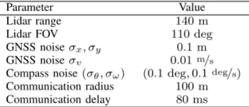
TABLE II

CHARACTERISTICS OF CAR SENSORS AND COMMUNICATION DEVICES.

Parameter Value

Lidar range 140 m

Lidar FOV 110 deg

GNSS noiseσx, σy 0.1 m

GNSS noiseσv 0.01m/s

Compass noise(σθ, σω) (0.1 deg,0.1deg/s) Communication radius 100 m Communication delay 80 ms

automotive modules developed in our laboratory.1 _Three

Citro¨en C-ZERO cars have been placed on an infinitely long, straight road with four lanes. The carEis placed behind the

carL, both facing one direction, whereas the carOfaces the

opposite direction and finds itself on the passing lane of the carE. The longitudinal positions of the three cars are random

in each experimental run, but their configuration remains as explained.2 Our algorithm could easily be adapted for curved roads by computing the distance in the road (curvilinear) coordinate system.

The cars E and L are traveling with target speeds v0

of 90 km_/_h _and ₅₀ km_/_h_{, respectively. They are equipped}

with a forward facing Ibeo LUX lidar sensor, generic GNSS and compass sensors achieving RTK performance, and a communication transceiver. Communication is achieved by simple messages implemented in the simulator environment using constant delay and message loss. The characteristics of integrated devices are listed in Table II. The carOtravels

at target speed of30km_/_h_{and is not equipped neither with}

sensing nor communication devices. Using higher traveling speeds would require using sensors with larger range.

The vehicle model implemented in Webots uses the throttle, brake, and steering angle as inputs. The input steering angle (provided by the lateral controller) is transferred to the wheels using a Webots built-in PID controller. We use the Citro¨en C-ZERO engine model3 _{to map the required acceleration}

(provided by the longitudinal controller) to the throttle input of the Webots car library, and we assume a linear brake response in the case of deceleration. The simulation step is

80 ms, equivalent to the sampling frequency of the lidar.

1_{For more details see http://disal.epfl.ch/RO2IVSim.}

2_{A video showcasing different experiments can be viewed at} http://disal.epfl.ch/NetworkedIV

3_{Provided by PSA Groupe.}

B. Tracking parameters

In the C-GM-PHD filter, we empirically determine the sensor standard deviation to be σz = [σx, σy, σθ]> =

[1 m,1 m,45 deg]> (this includes the point cloud pre-processing noise). To make our filter conservative, the ego state estimation noise needed for the Approximate Transformation is intentionally not set exactly to the values used in the simulator (cf. Table II). Instead, it equals to

[σx, σy, σθ, σv, σω]> = [1 m,1 m,0.5 deg,1m/s,0.5deg/s]>.

The clutter model is assumed to be Poisson with mean of

10 clutter measurements per sensor surveillance area. The probability of detection and survival are respectively set to

0.98 and0.99. The occlusion model, as well as the values of other parameters intrinsic to the C-GM-PHD filter are the same as in our previous work [2].

C. Experimental results

The experiments are conducted using six different pa-rameter settings. While keeping the value ofTstart at some

small, positive value (we chose 0.01), we vary Tabort ∈ {0.2,0.5,0.8}. For each value of Tabort, we launch the

experiment with and without cooperative fusion. Without fusion, the carEtracks targets using only its lidar, thus having

shorter range and more occluded FOV. For each of the six settings we perform500simulation runs with different random initial positions to obtain statistically significant results.

An overtaking attempt is defined as an event in which the car _Estarts changing the lane. It can be finished by a successful overtake, an abort or a crash.

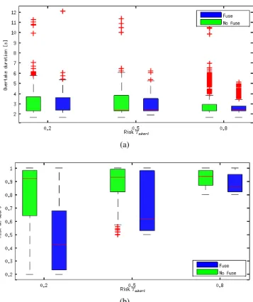
Fig. 4a shows the duration of overtaking maneuver, measured from the moment the first overtaking attempt is made (excluding experiments that resulted in crashes). Long durations represent overtaking maneuvers whose first attempts have been aborted, as in these cases the car Ehad to wait

for the risk to diminish before starting and successfully completing the second overtaking attempt. It can be seen that the duration decreases with increased risk threshold Tabort.

This is due to overtakes that are less likely to be aborted, for the price of accepting more risk. We can also see that experiments which use fusion outperform the ones without fusion algorithm: since, when using fusion, the car_E suffers less from occlusions and can see further away, it aborts the overtaking attempt less frequently and therefore saves time. The percentage of aborted overtakes is given in Table III. Aborts are split in two categories, the ones in which the carE

brakes and pulls behind the carL, and the ones in which the

carE keeps accelerating and successfully finishes the risky

maneuver. There are significantly less aborts of the second type in the case of fusion than in the case of no fusion. Their number also decreases with the increasingTabort, as the carE

allows for higher risk before aborting. Due to larger sensor range in the fusion case, there are slightly more aborts of the first type than in cases without fusion. These facts lead us to the conclusion that cooperative fusion might contribute to road safety, as it reduces the number of occasions in which the overtaking car enters risky situations. Fig. 4b supports this conclusion, by showing the actual risk at which the overtaking

(6)

(a)

(b)

Fig. 4. Boxplots showing for different values ofTabort(a) overtake duration from the moment of the first overtaking attempt, (b) overtaking risk at abort (note: the risk is always higher or equal than the abort thresholdTabort). Each box aggregates500runs minus the number of crashes and represents the upper and lower quartiles, the red line in the box marks the median, the bars extend to the most extreme data points not considered outliers, and the red crosses show outliers.

TABLE III

PERCENTAGE OF ABORTED AND CRASHED OVERTAKES. Risk

0.2 0.5 0.8

No fuse Fuse No fuse Fuse No fuse Fuse Abort behindL (%) 2.47 3.58 2.24 4.25 2.93 3.18 Abort in front ofL (%) 16.29 0.42 9.39 0.21 7.53 0.21 Crash (%) 1.62 0.00 1.01 0.00 2.65 0.81

maneuver was aborted. It is always significantly lower in the case of fusion, independent from the chosen value of Tabort.

Overtakes resulting in a crash between the car _E and the car O are listed in Table III as well. Data show that

cooperative fusion successfully reduces the number of crashes with the oncoming car, which is indeed its intended purpose. As expected, the highest number of crashes are recorded for

Tabort= 0.8.

VI. CONCLUSION

We presented a novel overtaking decision algorithm for intelligent vehicles which relies on the C-GM-PHD filter. By using information provided by the filter, the algorithm assesses the risk of overtaking (i.e., the risk of an oncoming car being on the passing lane within the collision distance

from the ego car). We compared the cases in which the leading car cooperates with the ego car by sharing its track estimates, and in which it does not. The overtaking algorithm showed good performance and the added value of cooperative fusion was evident from the experimental data. The number of risky maneuvers was significantly reduced when the ego car benefited from the higher sensor range, less occlusions and higher tracking confidence. Due to lower risk, the number of crashes between the ego and the oncoming car was also lower. When the cooperative fusion algorithm was used, a smoother and safer vehicle operation was noticeable.

As future work, one could consider more complex eval-uation scenarios, such as those characterized by additional traffic traveling on multiple lanes in different directions, or having different traffic participants in addition to cars (e.g., trucks, bikes). Moreover, the tracking algorithm would need to be extended to address the object detection problem in more complex scenarios.

REFERENCES

[1] “Traffic Safety Facts 2013: A compilation of motor vehicle crash data from the fatality analysis reporting system and the general estimates system,” NHTSA, DOT HS 812 139, 2013.

[2] M. Vasic and A. Martinoli, “A collaborative sensor fusion algorithm for multi-object tracking using a Gaussian mixture Probability Hypothesis Density filter,” inIEEE Intelligent Transportation Systems Conference, 2015, pp. 491–498.

[3] R. Toledo-Moreo, J. Santa, and M. A. Zamora-Izquierdo, “A cooperative overtaking assistance system,” inIros 2009 3rd Workshop: Planning, Perception and Navigation for Intelligent Vehicles, 2009.

[4] A. Vinel, E. Belyaev, K. Egiazarian, and Y. Koucheryavy, “An overtaking assistance system based on joint beaconing and real-time video transmission,” IEEE Transactions on Vehicular Technology, vol. 61, no. 5, pp. 2319–2329, Jun. 2012.

[5] W. Birk, E. Osipov, and J. Eliasson, “iRoad - cooperative road infrastruc-ture systems for driver support,” in16th World Congress and Exhibition on Intelligent Transport Systems, 2009. ISBN 978-1-61738-589-6 [6] B.-N. Vo and W.-K. Ma, “The Gaussian mixture probability hypothesis

density filter,”IEEE Transactions on Signal Processing, vol. 54, no. 11, pp. 4091–4104, Nov. 2006.

[7] B. Ristic, D. Clark, and B.-N. Vo, “Improved SMC implementation of the PHD filter,” in13th Conference on Information Fusion, Jul. 2010. doi: 10.1109/ICIF.2010.5711922

[8] G. Battistelli, L. Chisci, C. Fantacci, A. Farina, and A. Graziano, “Consensus CPHD filter for distributed multitarget tracking,”IEEE Journal of Selected Topics in Signal Processing, vol. 7, no. 3, pp. 508–520, Jun. 2013.

[9] M. Uney, D. Clark, and S. Julier, “Distributed fusion of PHD filters via exponential mixture densities,”IEEE Journal of Selected Topics in Signal Processing, vol. 7, no. 3, pp. 521–531, Jun. 2013.

[10] M. Ester, H.-P. Kriegel, J. S, and X. Xu, “A density-based algorithm for discovering clusters in large spatial databases with noise,” in International Conference on Knowledge Discovery and Data Mining, Portland, Oregon, USA, 1996, pp. 226–231.

[11] R. C. Smith and P. Cheeseman, “On the representation and estimation of spatial uncertainty,”The International Journal of Robotics Research, vol. 5, no. 4, pp. 56–68, Dec. 1986.

[12] R. P. S. Mahler, “Optimal/robust distributed data fusion: a unified approach,” inSignal Processing, Sensor Fusion, and Target Recognition IX, vol. 4052, 2000, pp. 128–138.

[13] A. Kesting, M. Treiber, and D. Helbing, “Enhanced intelligent driver model to access the impact of driving strategies on traffic capacity,” Philosophical Transactions of the Royal Society A, vol. 368, pp. 4585–4605, 2010.

[14] M. Treiber, A. Hennecke, and D. Helbing, “Congested traffic states in empirical observations and microscopic simulations,”Physical Review E, vol. 62, no. 2, pp. 1805–1824, 2000.