DigitalCommons@University of Nebraska - Lincoln
Computer Science and Engineering: Theses,Dissertations, and Student Research Computer Science and Engineering, Department of
Fall 12-2018
Reducing the Tail Latency of a Distributed NoSQL
Database
Jun Wu
Follow this and additional works at:http://digitalcommons.unl.edu/computerscidiss Part of theComputer Engineering Commons, and theComputer Sciences Commons
This Article is brought to you for free and open access by the Computer Science and Engineering, Department of at DigitalCommons@University of Nebraska - Lincoln. It has been accepted for inclusion in Computer Science and Engineering: Theses, Dissertations, and Student Research by an authorized administrator of DigitalCommons@University of Nebraska - Lincoln.
by
Jun Wu
A THESIS
Presented to the Faculty of
The Graduate College at the University of Nebraska In Partial Fulfillment of Requirements
For the Degree of Master of Science
Major: Computer Science
Under the Supervision of Professor Lisong Xu
Lincoln, Nebraska Dec,2018
Jun Wu, M.S.
University of Nebraska, 2018
Adviser: Dr. Lisong Xu
The request latency is an important performance metric of a distributed database, such as the popular Apache Cassandra, because of its direct impact on the user experience. Specifically, the latency of a read or write request is defined as the total time interval from the instant when a user makes the request to the instant when the user receives the request, and it involves not only the actual read or write time at a specific database node, but also various types of latency introduced by the distributed mechanism of the database. Most of the current work focuses only on reducing the average request latency, but not on reducing the tail request latency that has a significant and severe impact on some of database users. In this thesis, we investigate the important factors on the tail request latency of Apache Cassandra, then propose two novel methods to greatly reduce the tail request latency. First, we find that the background activities may considerably increase the local latency of a replica and then the overall request latency of the whole database, and thus we propose a novel method to select the optimal replica by considering the impact of background activities. Second, we find that the asynchronous read and write architecture handles the local and remote requests in the same way, which is simple to implement but at a cost of possibly longer latency, and thus we propose a synchronous method to handle local and remote request differently to greatly reduce the latency. Finally, our experiments on Amazon EC2public cloud platform demonstrate that
our proposed methods can greatly reduce the tail latency of read and write requests of Apache Cassandra.
DEDICATION
This thesis is dedicated to my family, for their continuous and warm encouragement and support through my way to the degree.
ACKNOWLEDGMENTS
I would first like to thank my thesis advisor Dr. Lisong Xu of Department of Computer Science & Engineering at University of Nebraska Lincoln. His excellent forethought and guidance inspire me a lot. He is always there if I encountered any problem. Without him, it could not be possible for me to complete this thesis. No words could describe how grateful I am for having him as my advisor.
Meanwhile, I would also like to thank my committee members, Dr. Hongfeng Yu and Dr. Qiben Yan for serving as my committee members. Greatly thanks them for generously offering their time, support, and guidance throughout the preparation and review of my thesis.
Lastly, I would like to say thanks to my family and my girlfriend. They offer uncondi-tional support and provide solid backing. When I was down, they’ll always be there and cheer me up. Without support from them, I could not be who am I today. Lastly, I would like to thank all my colleagues and my friends. We talk, we play together, we help each other, we share tears and laughter. My life could not be so wonderful without them.
Contents
Contents v
List of Figures vii
List of Tables ix
1 Introduction 1
1.1 Motivation . . . 1
1.2 Problem studied in this thesis . . . 3
1.3 Contributions . . . 5
2 Background 7 2.1 Key concepts and architecture in Cassandra. . . 7
2.2 Write path in Cassandra . . . 8
2.3 Read path in Cassandra . . . 11
2.4 Staged Event Driven Architecture (SEDA) . . . 12
3 Related Work 15 3.1 Research related to tail latency reduction . . . 15
4 Problems and Methods 21
4.1 Problem statements . . . 21
4.2 Problem analysis . . . 27
4.2.1 Small data set analysis . . . 28
4.2.2 Large data set analysis . . . 37
4.3 Approach to reduce tail latency . . . 46
4.3.1 Optimized replica ranking . . . 47
4.3.2 Local read improvement at coordinator node . . . 51
5 Evaluation and Results 55 5.1 Experiment set up . . . 55
5.2 Experiment Results . . . 57
5.2.1 Impact of data set size . . . 57
5.2.2 Impact of request distribution . . . 59
5.2.3 Impact of skewed record size . . . 64
5.2.4 Impact of workload on load condition . . . 66
6 Conclusion and Future Work 68 6.1 Conclusion . . . 68
6.2 Future Work . . . 69
List of Figures
2.1 Write request in a single data center cluster (adapted from [16]) . . . 9
2.2 Internal write path (adapted from [10]) . . . 10
2.3 Read request in a single data center cluster (adapted from [16]) . . . 11
2.4 Internal read path (adapted from [9]) . . . 12
2.5 A read request stage flow (adapted from [15]) . . . 13
4.1 Remote read path . . . 23
4.2 Local read path . . . 24
4.3 Requests received per 100ms . . . 25
4.4 Latency components in remote read . . . 28
4.5 Latency for small data set . . . 29
4.6 Latency ECDF for small data set . . . 30
4.7 Latency PMF for small data set . . . 31
4.8 Latency components breakdown for small data set . . . 32
4.9 Service time for small data set. . . 33
4.10 Service time ECDF for small data set . . . 34
4.11 Service time PMF for small data set . . . 35
4.12 Response time ECDF for small data set . . . 36
4.14 Latency for large data set . . . 38
4.15 Latency ECDF for large data set . . . 39
4.16 Latency PMF for large data set . . . 40
4.17 Latency components breakdown for large data set . . . 41
4.18 Service time for large data set . . . 42
4.19 Service time ECDF for large data set . . . 43
4.20 Service time PMF for large data set. . . 44
4.21 Response time ECDF for large data set. . . 45
4.22 Response time PMF for large data set . . . 46
4.23 Waiting time PMF for large data set . . . 47
4.24 Server ranking . . . 48
4.25 Server status exchange . . . 51
4.26 Local/remote requests co-exist . . . 52
4.27 Async/sync execution of read requests for Coordinator node . . . 53
5.1 Read latency comparison with small data set in Zipfian distribution . . . 57
5.2 Throughput characteristic comparison with small data set in Zipfian distribution 58 5.3 Selection results of Uniform and Zipfian [28] . . . 59
5.4 Read latency comparison with large data set in Zipfian distribution . . . 60
5.5 Throughput characteristic comparison with large data set in Zipfian distribution 61 5.6 Read latency comparison with large data set in Uniform distribution . . . 62
5.7 Throughput comparison with large data set in Uniform distribution . . . 63
5.8 Write latency comparison with large data set in Zipfian distribution . . . 64
5.9 Write latency comparison with large data set in Uniform distribution . . . 65
5.10 Read latency comparison with skewed data size . . . 66
List of Tables
4.1 Workloads in YCSB [28] . . . 26
4.2 Latency information for different workload patterns . . . 26
5.1 Experiment parameters . . . 56
Chapter
1
Introduction
1
.
1
Motivation
Relational database management systems (RDBMS) [20] have been traditionally used for organizing data. A RDBMS allows users to create, query, update, and delete databases. Hence, users can manage databases with the four corresponding basic operations: create, read, update and delete (known as CRUD) [38]. However, in the new ear of the Internet, challenges arise for the RDBMS with the need to manage very large data sets, which we call big data [44]. Because RDBMS were originally designed to work on a single machine as a server, the performance comes to a bottleneck to handle large data sets [26]. Hence, NoSQL (Not-only-SQL, also called non SQL) databases [45] are designed to solve this problem, while providing great performance.
As of today, NoSQL databases have been widely used for storing large data. These databases include Apache Cassandra [1], Apache HBase [3], MongoDB [11] etc. Compared with traditional RDBMS, like MySQL [12], Oracle [13], NoSQL systems are more powerful. Firstly, NoSQL systems are normally not centralized and distributed applications [33]. They are designed in a masterless fashion and there are no master-slave concepts proposed
in RDBMS. This property makes NoSQL systems easier to scale up horizontally [54]. Basically, we only need to add more machines/nodes to the systems and they can spread data automatically across multiple nodes. This could linearly improve the system capacity. Secondly, compared with RDBMS, the NoSQL systems support not only the structured data, but also the semi-structured and unstructured data. Hence, the NoSQL systems can support various types of data, like video, email, texts etc, while RDBMS can only handle
clearly defined data [57]. Meanwhile, for RDBMS, the schema should be predefined
before any operation, while NoSQL system can deal with dynamic schema. This provides more convenience to our current daily usage. Finally, for RDBMS, they are prone to server failures, because if the master node fails, the whole system will fail. However, NoSQL systems spread data among multiple nodes, even if one or more nodes go down, they still could provide continuous availability to the users [58].
Among these NoSQL systems, Apache Cassandra is one of the most representative ones. It’s free and open-sourced [62]. Currently, it is in use at eBay, Instagram, Netflix and many other companies [2]. In Cassandra, there is no master-slave concept and every node in the cluster is identical. Normally, data is stored in multiple nodes, working as replicas for fault-tolerance. Meanwhile, replication [59] across multiple data centers is also supported to geographically distribute data. Even an entire data center goes down, Cassandra is still able to provide service to users. So there is no single point of failure for the whole system [33]. Also, its elastic characteristic makes it easy to scale the system, by adding more new nodes. This could linearly improve the read and write throughput, without interruption to the existing applications [23].
The performance of Cassandra has a great impact on the user experience, especially the performance of the basic operations, such as write, read and delete. Among the performance metrics, the response time [32] is the most intuitive one for the users. Formally, it’s defined as the request latency or end-to-end latency, which is normally
the time duration from the time when an user sends out a request to the time when the user gets the operation results. Google [29] suggests that the request latency should be no more than100 ms to provide satisfactory user experience. Otherwise, the degraded
performance could directly impact revenues for the companies [22].
Therefore, in this thesis, we focus on analyzing the request latency problem [39] in Cassandra.
1
.
2
Problem studied in this thesis
There are two types of request latency. One is the average latency or the mean latency, and the other is the percentile latency, such as the99th percentile latency or even99.9th
percentile latency [65]. A recent measurement study [36] shows that the 95th (99th)
percentile latency of over 30% of examined services could be three times or even five
times of the median latency. Another measurement results of a Google service [29] show that the99th percentile latency is10 ms for a single random request.
However, the 99th percentile latency for all the requests to finish is140ms, while for
95% of the requests, that latency is only 70 ms. This means for the latency, 95% of the
requests are doubled, due to waiting for the remaining5% of the requests. These results
clearly show the importance of the percentile latency, which normally is called the tail latency [69]. Thus, in this thesis, we study how to reduce the tail latency. However, this could be quite challenging because of various reasons.
Firstly of all, Cassandra is a multi-tiered, distributed system, where a read request experiences more complex processes/stages than a write request. For example, a read request may experience the READ stage, READ RESPONSE stage, READ REPAIR stage in the whole read process [61]. Generally, reading data from the cluster may involve multiple nodes. For example, it may have connections among coordinator node, non-coordinator
node and the client machine. Nearly every node could potentially impact the tail latency performance.
Meanwhile, on each server, multiple applications are competing for the limited system resources, like CPU cores, memory and disk [42]. Even for a single application, these resources are shared among multiple stages. At the same time, as a distributed system, the nodes in Cassandra also need to compete for the network resources, such as the shared file system and the bandwidth of the network. This also adds unpredictable factors to the system [63].
Furthermore, for each server, background activities happen irregularly, which may also have unpredictable influence on the performance of the servers. Internally, this includes periodic garbage collection [43] activities in garbage-collective programming languages, such as Java. In the full Garbage Collection, applications may experience stop-the-world phenomenon. This could stop any other applications which are running on the Java Virtual Machine (JVM) platform [56]. Only after the completion of the full Garbage Collection, other processes could resume to normal status. Also, background data compaction could also happen during user’s requests. Data compaction is utilized to compact multiple SSTables to single one, which could incur a large number of disk I/O operations [40].
Finally, the hardware power of each server is limited [29]. Such limitations make it impossible to provide consistent high performance for Cassandra.
In summary, the complex design of Cassandra makes latency appear in multiple stages. The unpredictable background activities in each node make it hard to select the best replica. Meanwhile, limited hardware and network resources lead to the bottleneck for the system performance. All these factors contribute to the high latency in Cassandra cluster, especially the tail latency. The ultimate goal of this thesis is to study the impact of these factors on the tail latency and propose techniques to reduce the tail latency of
the whole cluster.
1
.
3
Contributions
This thesis makes the following contributions.
Firstly, we conduct a comprehensive measurement study to understand the reasons for the long tail latency. Specifically, we measure the queue size in the READ stage, the service time for each read request, the corresponding response time back to the coordinator node, and the waiting time in the queue that plays a very important part in the latency when the dataset size is large. For the queue size and service time, they’re measured both locally and remotely at their coordinator nodes. For the local read in coordinator nodes, these metrics are measured locally, while for the remote read for non-coordinator nodes, these metrics are measured in the non-coordinator nodes and piggy-backed to the coordinator node through the response packet.
Second, we find that the selection of the replica to read data has a big impact on the tail latency, because a better replica could reduce not only the local latency at the replica, but also the overall latency of the whole database, because of the better load balance among the nodes in the database [49]. Therefore, we propose a novel replica selection algorithm to select the best replica to read data from. This new algorithm considers the current status of each node and does not select the replica with busy background
activities, such as Garbage Collection and data compaction. Chapter 4 provides more
details for this algorithm.
Lastly, we modified the process for the case when local read and remote read exist, which helps reduce latency. In Cassandra, it uses Staged Event Driven Architecture (SEDA) [67], operations like read or write are put into multiple stages. Specifically for the read request, it includes the READ stage, RequestResponse stage, and ReadRepair
stage. These stages are modeled as a thread pool and the requests are executed by threads concurrently. Because of the multi-threading mechanism, Cassandra provides very powerful service in case of a large number of requests. For a read request, it could be served locally by its coordinator node or remotely by a non-coordinator node. For the local service, it’s still using the READ stage to execute the local read asynchronously. In this case, when there are multiple requests waiting for available threads, this could lead to a large amount of waiting time for the request. Meanwhile, the switch time of different stages could also add unnecessary latency. Based on this observation, we can reduce this part of waiting and queuing latency, by modifying the local read process, and letting the local read to be executed synchronously in the request thread.
Chapter
2
Background
In this chapter, the basic but important concepts in Cassandra are introduced firstly. Then, we present the flow for both the write path and read path. Finally, we introduce the architecture that Cassandra is built on.
2
.
1
Key concepts and architecture in Cassandra
Apache Cassandra was originally designed at Facebook. Afterwards, it combines the features from Amazon’s DynamoDB [30] and Google’s BigTable data model [25]. Since then, it becomes a top-tier project. Essentially, Cassandra is a key-value based database [53], which means that it has a primary key connecting with a set of data. This key is used for data retrieval. According to the famous CAP (Consistency, Availability, Partition tolerance) theorem proposed by Eric Brewer [5], Cassandra typically falls into the AP system. That means Cassandra makes sure that every operation receives a response, no matter whether it’s successful or not. Meanwhile, it can continue working, even if part of the system goes down.
contrast, the Consistency level could be tuned by a replication factor and consistency level in Cassandra [18].
In Cassandra, nodes are the basic components to store data. When a client connects to one of the nodes to operate a read or write request, that node is served as the coordinator for the operation. A cluster is a group of nodes, which could be a single node, a single data center or multiple data centers [51].
To share each node’s information, Cassandra uses the peer-to-peer communication protocol called Gossip [19]. To assure no single point of failure [46], data is distributed among multiple nodes in the cluster. These nodes are called replica. A replication factor could be set up with various needs. For example, a replication factor of1 means there
is only one copy of each row in one node. A replication factor of3 means three copies
of each row and each copy is in a different node. We can set up the replica replacement strategy to be either SimpleStrategy or NetworkTopologysTrategy [52]. The former is used for single data center, while the latter is used for multiple data centers. A consistency level could also be configured with multiple choices, like ONE, TWO, THREE, etc [66]. It should be less than the number of nodes. Further, it could be set up to ANY, QUORUM. The default consistency level for both read and write requests is 1. For a write operation,
that means a write must be written to the CommitLog and MemTable of at least one replica. For a read request, it means the client should get one response from the closest replica.
2
.
2
Write path in Cassandra
Figure2.1shows the operation for the write request in a single data center cluster. The cluster consists of6 nodes and the replication factor is set to3. When a client wants to
Then, three copies of the data are written to nodes 3,4and5. If the consistency level is
set to the default value of 1, then only one node will send a write-success response back
to the Coordinator. Finally, the Coordinator sends back a write acknowledge to the client, telling it the whole write request is done.
Client 6 5 4 2 1 3 Coordinator node Replica node R1 R3 R2 Write request/response
Figure2.1: Write request in a single data center cluster (adapted from [16])
For a write path in Cassandra, the write request goes through multiple stages. Figure 2.2shows the full stage. For each column family, it may go to three different layers for storage: MemTable, CommitLog and SSTable (Sorted String Table). MemTable is a special structure in memory. It works similarly to a write-back cache of data, which can be looked up by the primary key. Commit log is a log structure in disk to store data. When new data needs to be written, it will be appended to Commit log, which is for durability. Even if the data in MemTable gets lost, it can still be recovered from the Commit log. Because the size of memory is limited, when the size of the MemTable reaches to its limit, data will be flushed to SSTable. Data in Commit log will be purged after the corresponding
data in MemTable is flushed to an SSTable. SSTable is immutable, which means after writing, it can’t be changed. For each SSTable, it maintains a partition index, a partition summary and a Bloom filter. All these structures are used for quicker read. A partition index is a list of partition keys and positions of data on disk. Partition summary is a sample of partition index [10].
SSTable
CommitLog
MemTable
Write request
Figure2.2: Internal write path (adapted from [10])
Meanwhile, as SSTables are immutable, the size of SSTables increases drastically. To save the space and assure updated data, Cassandra provides a mechanism called compaction to compact the SSTable periodically. Essentially, Cassandra compares the timestamps of the data and marks the outdated data that will be deleted later. Then updated data are accumulated into a new SSTalble during compaction.
2
.
3
Read path in Cassandra
The read path is more complex than the write path. In a single datacenter cluster illustrated in Figure 2.3, the replication factor is 3 and consistency level is one. The
closest replica is selected for full reading. Meanwhile, a read repair may happen in the background, based on the read repair chance parameter.
Client 6 5 4 2 1 3 Coordinator node Replica node R1 R3 R2 Read request/response
Figure2.3: Read request in a single data center cluster (adapted from [16])
Figure 2.4 shows the internal read process. When a read request comes in, a node checks the Bloom filter, which is a space-efficient probabilistic data structure designed to check whether an element is not inside a data set [4]. When the Bloom filter shows that data is not in the corresponding SSTable, it skips the scan for this SSTable. Then Cassandra checks the partition key cache and if the entry is found in the cache, it goes to the compression offset map and finds the position that has the data. If it’s not found in the cache, Cassandra goes to the partition summary to check the approximate location of
the entry. If the entry is still not found, then it goes to the partition index for full scan and finds the position for the data [9]. After finding the position of the data, then it fetches the data from the disk and returns the result back to the client.
Partition index Bloom filter
Partition summary Partition key cache
Compression offset
Data Return
data Read request
Figure2.4: Internal read path (adapted from [9])
2
.
4
Staged Event Driven Architecture (SEDA)
Cassandra is based on a Staged Event Driven Architecture (SEDA) [67]. This architecture is designed for highly concurrent Internet services and is intended to support massive concurrency demands. In SEDA, applications are composed by multiple event-driven stages, which are collected by message queues. This design provides high performance and is robust to dynamic load.
In Cassandra, different events correspond to different stages. For example, for a write request, it goes to Mutation Stage, while for a read request, Read Stage is allocated to handle it. Meanwhile, multiple other stages are included, such as the Request Response Stage, Internal Stage and Gossip Stage, etc [15]. Each stage has a thread pool and an event queue. The thread pool is to execute the current requests while the incoming request are queued in the event queue. When one of the threads is available, a request is removed from the event queue and moved to the available thread to be executed [14].
To demonstrate the process, take a read request as an example. For instance, node A wants to send out a read request to node B. The whole process may go through the process illustrated in Figure 2.5.
Thread Thread Thread
NodeA Read requests NodeB ReadStage NodeA RequestResponse NodeA ReadRepairStage queue queue queue
Figure2.5: A read request stage flow (adapted from [15])
Basically, these are the working flow: (1) Node A sends out a read request to node
B. The request is queued in the event queue of node B. (2). If one of the threads in the
queue and executed. (3). When the request has been executed, the result rows are fetched
and sent out to the Request Response Stage of node A. (4). Similarly, the thread pool of
node A executes the request response from node B and returns the result to the client. (5).
Meanwhile, the read repair operation is optional to be processed in node A. Note that in the figure above, the thread pool size for the Read Stage is set to 32, while the size for
Request Response Stage and the Read Repair Stage is 4. Actually, these are the default
Chapter
3
Related Work
3
.
1
Research related to tail latency reduction
There has been years of research on the tail latency reduction, especially in the cloud platform. Jeffrey Dean and Luiz Andre Barroso in Google introduced multiple techniques to reduce the latency [29]. They mentioned that there are multiple reasons for latency. High tail latency in individual components of a service could be caused by global resource sharing, maintenance activities, queueing and background activities. They provided high-level solutions based on both the short-term and long-term adaptions. Real time status of the servers are monitored. Then the client avoids the slowest server.
[36] is another paper to analyze the tail latency and provide solutions to the latency reduction. This paper analyzed the latency distribution in each stage of the web service of Bing. It found that the reasons for high latency includes slow servers, network anomalies, complex queries, congestion due to improper load balance, and software artifacts like buffering. Three techniques are developed to resolve the latency issue: reissues, incompleteness, and catch-up. The adaptive reissue is to get the time information from the past queries, and then start a second copy of the request at the optimized time
calculated using the statistics collected. The incompleteness method is to trade off completeness with latency. The catch-up technique allocates more threads to process the slow requests and uses high priority network packets for lagging requests to protect them from burst losses.
A. Vulimiriet al. in [64] argued that with the use of redundancy, latency especially the tail latency could be reduced. The paper proposed a very powerful technique through redundancy technique: initiate an operation multiple times, and use the first result which completes. It also introduced a queuing model of the query replication, and analyzed the expected response time as a function of the system utilization and server-side service time distribution. This technique showed great performance improvement on both the mean and tail latency reduction in several systems, such as DNS queries, database servers.
[68] focused on another aspect of tail latency reduction in the cloud platform. It
verified with experiments, showing that the poor response times in Amazon EC2 are
a property of nodes. The root cause for the long response time on each node is the co-scheduling of CPU-bound and latency-sensitive tasks. Then it implemented a framework called Bobtail to detect the instances of which the sharing processor does not cause extra long tail latency. Then users could use Bobtail to decide on which instance to run their latency-sensitive tasks. The final results showed that with the usage of Bobtail, the99.9th
percentile response time could be reduced by40 %.
[70] focused on scheduling requests to meet the service level objectives (SLO) for tail latency. It automatically configured workload priorities and rate limits among shared network stages. Through measurements, high priorities were used to provide less latency to the workloads which required low latency. If a workload can meet it’s SLO with a given low priority, then this lowest priority is removed from the search. Otherwise, it would iterate on the remaining workloads at the next lowest priority. Through this method, it assured each task is finished within the SLO constraint. Meanwhile, to prevent starvation,
multiple rate limiters were utilized for each workload at each stage.
Sh. Khan and ASML Hoque in [37] indicated that in data center applications, pre-dictability in service time and controlled latency, especially tail latency, were quite important to build high performance applications. It analyzed three data center applica-tions: Memcached, OpenFlow and Web search, to measure the effect of1) kernel socket
handling, NIC interaction, and the network stack,2) application locks in kernel, and 3)
application queuing due to requests queued in the thread pool. It proposed a framework called Chronos to deliver low-latency service in data center applications. Chronos utilized user-level networking APIs to reduce lock contention and perform efficient load balancing. The experiments results showed that, the tail latency of the new Memcached with the Chronos could be reduced by a factor of20, compared with existing Memcached.
J. Li et al. in [41] explored the hardware, OS, and application-level sources of high tail latency in high throughput servers in multi-core machines. It modeled these network services as a queuing system, to establish the best latency distribution. Using fine-grained measurements, it showed that the underlying causes for the high latency include interference from background tasks, request re-submit due to poor scheduling, sub-optimal interrupt routing, etc. To fix those problems, it implemented several mechanisms. For example, it either used real-time scheduling priorities or isolated threads on dedicated cores, to isolate the server from background tasks. The final experiments showed that it reduced the 99.9th percentile latency of Memcached from5ms to32us at 75% utilization.
M. Haqueet al. in [34] proposed a mechanism called Few-to-Many(FM) incremental parallelization, which dynamically increases parallelism to reduce tail latency. It used request service demand profiles and hardware parallelism in an offline phase to compute a policy. This policy is to specify when and how much software parallelism to add. Then during running time, FM adds parallelism. If a request executes for a long time, then FM adds more parallelism. The result showed that FM reduces the99th percentile response
time up to26% in Bing and 32% in Lucene.
3
.
2
Performance research related to Cassandra
Because Cassandra has been popularly used only in recent years, there is very little research on the performance research.
Paper [24] described the architecture of a QoS infrastructure for achieving controlled application performance over Cassandra. It tried to fix the storage configuration problem. Meanwhile, it could also address the dynamic adaption problem, by monitoring service performance at run time and adjusting the short term variations. The core of the architecture is the QoS controller. This controller collected response time and throughput metrics periodically. Then it performed admission control, by estimating overall resource and level of sanctification of requirements.
In Cassandra, mixed query types existed, such as a single query to obtain just a value. Then in this case, a single query needed to wait for the completion of the range query, which took longer time than a single query. This caused the increase of theresponse time. Then S. Fukuda et al. in [31] proposed a query scheduling algorithm. It gave the higher priority to a single query and made the query be executed before a range query. For range queries, this algorithm also gave higher priority to queries which require fewer search results. The priority assignments were dynamically changed with the progress of query execution.
In [50], Sh. Nakamura and K.Shudo developed a modular cloud storage called
MyCassandra, based on Cassandra. To optimize the read the write performance, it built a storage engine interface, based on different types of storage engines, such as MySQL, Redis. When a query came in, the interface guided the query to different storage engines, based on whether the query is read-optimized or write-optimized. Through this
re-direction, the read and write latency could be reduced by leading the query to the nodes which process faster. The final results showed that MyCassandra could reduce the read latency by90% and improve the throughput up to11times in specific workload.
P. Suresh et al. in [60] aimed to cut the tail latency in Cassandra through adaptive replica selection. They proposed a new algorithm called C3. It focused more on the
read path and improved the read performance. Two mechanisms were proposed: replica ranking and distributed rate control. For the replica ranking, it modified the existing dynamic snitch algorithm, which only considered the history latency to decide the best replica to read data from. Additionally, C3 measured the queue size, the response time
and the service time for each server. Then it piggy-backed these information to the client, to let the client selects the best replica. Meanwhile, it measured the request served in a fixed time interval, then sent it back to the client. Then the client dynamically adjusted the request sending rate. The final result showed improvement on mean, median and tail latency. Specially, for the99.9% latency, there is a3 times improvement.
In [35], the authors formalized the write process model of Cassandra and explored two queuing systems: the sending task queue and mutation queue. The sending queue was defined as the queue in the coordinator node and the mutation queue was the queue to wait for mutation in both the coordinator and non-coordinator node. This paper modeled
the sending queue as a G/G/1 system and mutation queue as a G/G/S system. Then it
measured the inconsistency between two replicas via the departure time difference from the mutation queue. Furthermore, metrics like Request Per Second(RPS) were measured. Then through the measurement of the RPS, the Mutation Threads Number(MTN) was adjusted dynamically. Meanwhile, it also proposed a metric called inherent inconsistency time window(IITW), to measure the replica consistency.
W. Chow and N. Tan in [27] investigated the usage of redundant requests to reduce the read latency in Cassandra. It tested the system via a dynamical threshold when
sending duplicate requests. It also tried to change sending duplicate replies with a small portion. The results showed that these mechanisms performed similar to the average case and performed better in the long tails. Meanwhile, in order to dynamically determine the optimal retry threshold, the paper applied a graphical model to predict the network latency in the system. By exploring the correlation between nodes and time, the model was more accurate from the results.
J. Polo et al. in [55] explored the effects which additional consistency guarantees and isolation capabilities may have on the store state of Cassandra. It proposed a new multi-versioned isolation level which provided stronger guarantees. This isolation was implemented in the form of readable snapshots, which included changes in both the data store and the read path of Cassandra. Meanwhile, it implemented a new compaction strategy which compacted the SSTables only within certain boundaries. With this new compaction strategy, only specific SSTables were considered for compaction. The final results showed that it not only improved the throughput, but also the average read latency.
Chapter
4
Problems and Methods
4
.
1
Problem statements
In Apache Cassandra, data is stored among multiple replicas. To read data from the cluster, the client needs to contact one of the nodes, which works as the coordinator node. The coordinator node is the proxy between the client and the whole cluster. Through the coordinator, the client gets the information of the whole cluster. The client sends a request to the coordinator node and then the coordinator node gets the result or the acknowledge packet back to the client.
During this process, the coordinator node needs to select one or more replicas out of multiple replicas to serve a request. This is based on the consistency level (CL), determined by the users. The CL shows how up-to-date and synchronized of the data on all of the replicas and it could be any number between one and the total number of nodes. Cassandra extends the concept of eventual consistency by providing the tunable consistency level. For example, if we set the CL to be one, then one out of the replicas needs to send an acknowledge packet back to the coordinator node. If it’s two, then two out of the replicas need to reply back to the coordinator node. If the CL is large, then the
users could get more reliable data.
However, this could lead to long transmission latency, as the users need to wait for the acknowledge packets from a large number of replicas. On the contrary, if the CL is small, the performance for the latency could be guaranteed. Then the reliability of the data may vary. So the users should trade-off the settings with their own realistic requirement.
In this thesis, we consider the situation where CL is set to be one, which means the coordinator node needs to select one out of multiple replicas. One of the reasons for this choice is that we care more about the performance of latency in this thesis, not the data reliability. So having less replica to select from could reduce the latency greatly. In addition, setting the CL to be one is also a very popular tuning policy, which provides the data to the users in less time. So, to keep the design simple, the CL is set to be one in this thesis and the tunable consistency setting could be left for future work.
While the status of each replica is unknown, then how to select the best replica is a problem. For example, a potential replica may experience an unknown problem and could not serve the request. Or the replica itself may experience some background activities and could only provide very slow service. So this uncertainty of each replica makes the replica selection much more challenging. In this thesis, we care more about the performance of the latency, then the best replica means the one, which could provide the fastest service. In the later section, it shows that the replica selection has great impact on the latency distribution, especially the tail latency. As a distributed system, Cassandra is popularly deployed in cloud environments, such as Amazon AWS or Google Cloud, which experience much more resource contention and other uncertainties. This could further aggravate the performance fluctuation.
Meanwhile, each replica exhibits performance fluctuations over time. This makes the replica selection a challenging problem. At the same time, the coordinator could not always choose the fastest replica to service the requests and this could lead to the
herd behavior problem [48]. Herd behavior means multiple clients send requests to the fastest/best replica, which could cause the load imbalanced and further degrade the server’s performance. This could happen subsequently and cause the clients to choose other different nodes and repeat the same process.
In Cassandra, a snitch determines which data center nodes belong to and inform the Cassandra nodes about the network topology. Then the requests could be routed efficiently. Multiple snitches could be chosen according to user’s requirements. Among these snitches, one is called Dynamical Snitching, which is designed to make replica selection decisions. Dynamical snitch is wrapped on other snitches by default and working for the read side only. It monitors the read latency for each node and provides this information to the coordinator node. Then the coordinator node attempts to avoid the poorly-performing nodes.
Taking a 6-node Cassandra cluster as an example, as shown in the Figure4.1, when the client sends a request to the cluster, node1is selected as the Coordinator node. Node3,
node4, node5 are the three replicas which store the data.
Client Cluster 6 5 4 2 1 3 Coordinator node Replica node
Selected replica node R1
R3 R2
Read request/response
Since node1has the latency information of each replica node, node3is selected to read
data from if it has the lowest latency. We call this process as a remote read.
Also, it could be possible that the coordinator node is one of the replicas. Then definitely we’ll choose this node to read data from. This process is called a local read, as shown in the Figure 4.2.
Client Cluster 6 5 4 2 1 3 Coordinator node Replica node
Selected replica node
R1
R3 R2
Read request/response
Figure4.2: Local read path
However, the performance is poor when making replica selection decisions based only on the latency information of each node. In our experiments, we’ve measured the requests served in a 6-node cluster, which is deployed in the cloud platform of Amazon EC2(the
settings are the same as those used in the experiment result chapter). In particular, we tracked the number of read requests served in each100ms interval.
The figure below shows that the default Dynamical Snitch is not working well and as a result the load varies a lot. The y-axes shows the number of read requests processed every100 ms for one node. It ranges from 1 up to 28 requests per 100 ms. Especially
sometimes the number of read requests processed in100 ms is only1, which means the
node is very busy at that time.
0 1 2 3 4 5 6 7 8 Time (seconds) 106 0 5 10 15 20 25 30
Requests received per 100ms
Load oscillations
Figure4.3: Requests received per 100ms
In addition to the vast load variance, other performance also experiences fluctuations, such as the latency, especially the tail latency, like99th,99.9th,99.99th percentile latency.
Dean [29] lists various sources for these latency fluctuation on Google cloud service. The phenomenon of long tail latency also happens in Apache Cassandra, because of the reasons mentioned in previous chapters and demonstrated below.
To demonstrate the long tail latency phenomenon in Apache Cassandra, a tool called YSCB (Yahoo! Cloud Serving Benchmark) [28] is used. YCSB is one of the most popular tools to evaluate and benchmark various databases, including both traditional databases and NoSQL databases. In YCSB, multiple workload patterns could be used to generate
customized workloads with different requirements. In our thesis, we care more about the read performance, so we use three workloads: update heavy, read heavy and read only. The operations in update heavy workload include 50% of read and 50% of update. The
operations in read heavy workload include95% of read and5% of update. The operations
in read only workload are all read. These three workloads are generated with the Zipfian or Uniform distribution.
Workloads Operations Distributions
A - Update heavy Read: 50% Update: 50% Zipfian/Uniform
B - Read heavy Read: 95% Update: 5% Zipfian/Uniform
C - Read only Read: 100% Zipfian/Uniform
Table 4.1: Workloads in YCSB [28]
With the same settings, we conduct experiments to get the tail latency information through YCSB. In these experiments,6nodes form a cluster. SimpleStrategy is used for
the replication strategy and the replication factor is set to3. Zipfian distribution is used
for the workloads with4 Gb data. Table 4.2shows the latency performance regarding the previous three workloads, including average, min, max, 95th, 99th, 99.9th, 99.99th
percentile latency. The unit for latency in the table is milliseconds.
Workloads vs Latency average min max 95th 99th 99.9th 99.99th
A - Update heavy 3.09 0.54 91.19 5.76 8.44 15.56 32.30
B - Read heavy 2.37 0.48 215.30 4.46 5.86 11.62 22.59
C - Read only 2.59 0.44 235.14 4.40 7.54 12.22 33.37
Table 4.2: Latency information for different workload patterns
From Table 4.2, we can see the vast gap between the average latency and the tail latency. Taking the result of read-only workload as an example, minimum latency is
0.44ms, and the maximum latency goes up to 235.14 ms, which must experience long
latency is 33.37ms, which is nearly10X times of the average latency. Also, the difference
between the 95th,99th,99.9th values are also large. This long tail latency happens in all
three different workloads, which could further influence the end-user delay. Below we investigate the reasons for the long tail latency and seek solutions to effectively reduce the tail latency.
4
.
2
Problem analysis
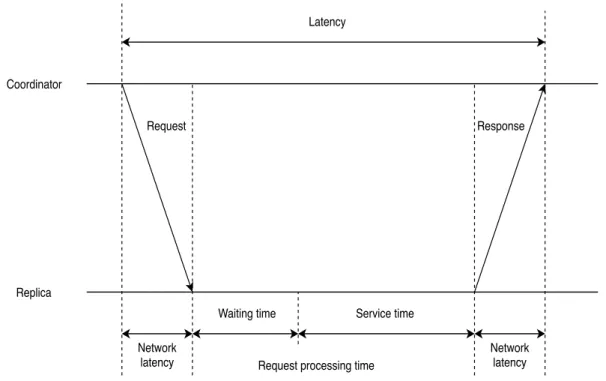
In read request processing, the read latency could be divided into several components. Taking a remote read request as an example, when the Coordinator node decides the replica and sends out a read request, there’s a request time, which is basically the network latency between the two nodes. Since the request time is relatively small, it can be ignored.
Our experiment showed that the RTT(round-trip time) time between two nodes in the same rack is0.75ms in average, with the packet size64 bytes. The max RTT time is
about1.59 ms, which is still relatively small compared with the whole latency. Actually
in our experiments, this part is ignored when it’s a local read, since there’s no cross node connection. When the request comes to the replica and the replica needs to process the request and retrieve data from its memory or disk, this part is called the request process time. Based on the status of each replica, this process time could vary a lot and contributes majority to the whole latency. Specifically, the process time includes both the waiting time in the queue and the real service time for each request. Figure4.4shows the latency components for the remote read operation. We’ll analyze each component in the part below.
Finally, after finishing the read process, the replica needs to send the data back to the Coordinator if it’s a remote read process. The response time is also one of the important
parts in the latency, since the data we read could be quite large, like in Gigabyte unit.
Request processing time
Request Response Network latency Latency Coordinator Replica Network latency Waiting time Service time
Figure4.4: Latency components in remote read
To dig deeper into the internal components of the latency issue, we conduct experi-ments with different settings: small data set and large data set. Here small means the size of the data set (750 MB) is less than the RAM memory (1GB) of the server. In this case,
reading data only needs to access the memory for most situations. Only in very few cases, it needs to read data from disk. Large data set means the data set size (4 GB) is larger
than the memory size (1GB). In this case, it needs to access disk for every read request.
4
.
2
.
1
Small data set analysis
First of all, we start our experiments with a small data set, which consists of0.75million
data of records. The size of each record is1KB, and thus the total data size is750MB. The
total data size is less than the RAM memory of the experimental Amazon EC2instance,
unit. From the figure, we can see the latency varies a lot, from minimum value of0.26
ms to maximum value of 74.72 ms. The max value 74.72 ms is way out of the latency
range and is possible an anomalous value. With experiment going on, the latency for each request could still go as high as33 ms. Also, some of the requests could be served
in more than10ms, or even above 20ms.
Figure4.5: Latency for small data set
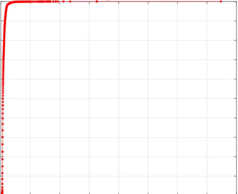
Furthermore, we plot the ECDF (Empirical cumulative distribution function) of the latency for one of the nodes as in Figure4.6. The x-axis is the latency value, while the y-axis is the ECDF value. The figure shows that the average latency is about 0.88 ms,
while the median latency is 0.68ms. The 95% percentile latency is about1.72ms, which
is about2.5times the median value. The99% percentile latency is about2.82ms, which is
is about 7.9times the median latency. The statistic shows the big variance of the latency
metric, while the tail latency contributes a lot. Also, we found the difference between the high percentile latency is large. For example, the 99.9% percentile latency almost doubles
the value of99% percentile latency and triples the value of 95% percentile latency.
0 10 20 30 40 50 60 70 80 x 0 0.1 0.2 0.3 0.4 0.5 0.6 0.7 0.8 0.9 1 F(x) Empirical CDF
Figure4.6: Latency ECDF for small data set
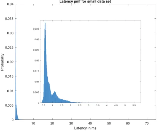
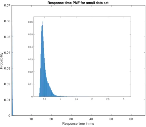
Figure4.7shows the PMF (Probability mass function) of the latency for the same node with small data set. To make the figure clearer, the zoomed plot has been added in the middle of the figure. From the figure we can see that, most of the latency lies between
0.5ms to 0.8ms, with0.58ms is the most frequent latency value. This latency is the first
peak in the figure. The reason behind the first peak is the read access to the memory. Since the data set size is less than the RAM memory. So for most of the read requests,
they can be served through reading data from memory only. Only for few times, if the data not in the memory, it will need to access the disk.
Figure4.7: Latency PMF for small data set
However, for few times, if reading from the memory fails, it will read data from disk as well. This comes to the second peak in the PMF figure. The latency for the second peak lies between0.96ms to 1.24ms. In this case, reading data needs to access the disk,
which causes a longer reading time.
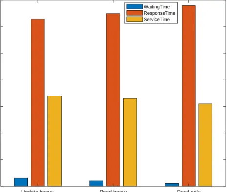
After further experiments, we found that the latency consists of different components. Figure4.8shows the latency components breakdown, which includes the waiting time in the queue, response time via the network latency, and service time to serve the request. The figure below shows the average ratio for each component with different workloads. The experiments show the response time is the major component for the latency, which
Latency components breakdown for small data set
Update heavy Read heavy Read only
0 0.1 0.2 0.3 0.4 0.5 0.6 0.7 Average ratio WaitingTime ResponseTime ServiceTime
Figure4.8: Latency components breakdown for small data set
takes more than half of the latency. Also the service time is the second important factor and it takes about 30% of the latency. Meanwhile, the waiting time in the queue only
takes about 3% in average. This is because the data set is small, read requests only need
to read from memory, which won’t take too long to process. Consequently, the network latency part dominates the whole latency.
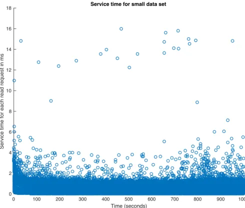
Figure4.9is the service time for each request on one of the nodes in the cluster. From the experiment result, we can see the service time varies a lot, ranging from the minimum value of0.03ms to the maximum value of16ms, while the average service time is about
0.33 ms.
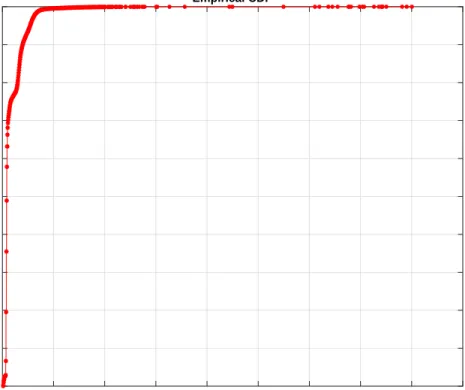
Figure4.10is the ECDF distribution plot for the service time in one of the nodes with the small data set. From the figure, we can see that the average value of the service time
0 100 200 300 400 500 600 700 800 900 1000 Time (seconds) 0 2 4 6 8 10 12 14 16 18
Service time for each read request in ms
Service time for small data set
Figure4.9: Service time for small data set
is0.33 ms and the median value is0.22ms.
However, when coming to the high percentile values, it shows the 95%, 99%,99.9%
percentile values are 1.08ms, 1.45 ms and3.51 ms respectively, which is4.9,6.6 and16
times of the median value.
Meanwhile, the big difference between the high percentile values also indicates the fluctuation of the service. The 99.9% percentile value doubles the 99% percentile value,
and triples the95% percentile value.
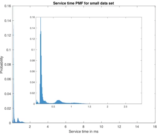
Figure 4.11 is the PMF for the service time with the small data set. From the statistic, it shows that most of the service time is less than 2ms. 74.6% of the service time is in
the range of0.11 ms to0.49ms, which is the first peak in the figure. The reason for this
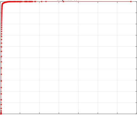
0 2 4 6 8 10 12 14 16 18 x 0 0.1 0.2 0.3 0.4 0.5 0.6 0.7 0.8 0.9 1 F(x) Empirical CDF
Figure4.10: Service time ECDF for small data set
read requests need only to access the memory. Another peak is in the range of0.51ms to
1.24ms. Similarly, this peak is occurred because of reading data from disk, when reading
data from the memory failed. Accessing data in disk also may cause unpredictable issues. From the figure we can see, the service time could go up to 16 ms. This significantly
increases the tail latency.
Because the response time takes the largest portion in the latency for the small data set, we analyze it below.
Figure 4.12and Figure4.13show the ECDF and the PMF plot for response time with the small data set. Even though the response time varies, ranging from the minimum value of 0.12 ms to the maximum value of66.97ms, the figure shows that the response
Figure4.11: Service time PMF for small data set
value matches closely with our previous experiments on the RTT time experiments between two nodes in the same rack.
0 10 20 30 40 50 60 70 x 0 0.1 0.2 0.3 0.4 0.5 0.6 0.7 0.8 0.9 1 F(x) Empirical CDF
Figure4.12: Response time ECDF for small data set
Figure4.12shows that the median response time is about 0.56ms, which is very close
to the average response time. The95%,99%, 99.9% percentile values are0.75ms,1.88ms
and4.2ms respectively, which are 1.3,3.4and7.5times of the median value. Most of the
response time is less than1ms. Actually from the PMF plot, the response time is closely
Figure4.13: Response time PMF for small data set
From the analysis above, we can see for the small data set, the latency distribution mainly depends on service time.
4
.
2
.
2
Large data set analysis
We’ve worked on a large data set with the data size of 4GB, which is greatly larger than
the RAM memory of1GB.
For the larger data set, since the data can not be fit into the memory any more, so reading data from the node requires accessing the disk to read the full data set. Figure4.14 shows the latency for each read request in a node with the millisecond unit. Compared with the small data set results, its value range varies even larger, ranging from the
minimum value of 0.22 ms to the maximum value of165.18 ms. The figure shows that
the peak latency value could go up to hundreds of milliseconds, which is definitely not tolerable in real time applications.
Figure4.14: Latency for large data set
Figure 4.15is the ECDF for the latency for one of the nodes with the large data set. It shows that nearly99% latency value is less than10ms, which means most of the requests
could be served within 10 ms. The average latency value is about 1.36 ms, while the
median latency value is 1.27ms. The95%,99%,99.9% percentile latency are 2.38ms,3.99
ms and 6.81ms, which are1.8,3.2and5.4times of the median latency value respectively.
The experiment results also show that the tail latency is pretty long, even the average latency values are a few milliseconds. Meanwhile, the differences between the high
percentile latency value is also very large. For example, the 99.9% percentile latency is
about1.7times of the99% percentile latency, and2.9 times of the95% percentile latency.
0 20 40 60 80 100 120 140 160 180 x 0 0.1 0.2 0.3 0.4 0.5 0.6 0.7 0.8 0.9 1 F(x) Empirical CDF
Figure4.15: Latency ECDF for large data set
Figure 4.16 shows the PMF for the latency. The first peak value of the latency is about 0.62 ms and the second, the third are around 1.18 ms and 1.62 ms respectively.
Similarly, the first peak value is the time to read data from the memory. If the data not completely stored in the memory, it will access the disk to read extra data from the disk. Reading data from disk is more time-consuming, which leads to the second peak in the figure. During the reading process, back ground activities like garbage collection, data compaction could happen. This further increases the time to read the whole data. When the background activities happen, the service to the read request could be stopped fully.
Figure4.16: Latency PMF for large data set
Similarly, we break down the components for the latency and analyze each component in it. Figure 4.17shows the average ratio for each component with different distribution workload. From the figure we can see the waiting time takes larger portion in the latency, compared with the small data set experiments. The average ratio of the waiting time over latency goes up to around8%. Meanwhile, the figure also shows that the service
time takes the largest portion in the latency, with the value around50%. This is because
the data size gets larger, then the chance of request congestion increases as well. Also, more background activities happen under-ground, such as garbage collection, and data compaction. These all could make the time to serve the request longer.
Among the latency, we conducted further experiments to measure the service time for each read request and found that the service time also varies a lot with an even larger
Latency components breakdown for large data set
Update heavy Read heavy Read only
0 0.1 0.2 0.3 0.4 0.5 0.6 Average ratio WaitingTime ResponseTime ServiceTime
Figure4.17: Latency components breakdown for large data set
range. Figure4.18below shows the measurement of the service time for each read request. It ranges from the minimum value of0.03ms to the maximum value of164.41ms, which
shows that the peak value could go up to hundreds of milliseconds. Compared with the average service time, it’s about 200times. This high value could contribute greatly to the
tail latency.
Similarly, we analyzed the distribution of the service time for the large data set. Figure 4.19shows the ECDF of service time for the large data set. The average and median values for the service time are0.79ms and0.72ms respectively, which are very close. Statistic
also shows that the95%, 99% and99.9% percentile values for the service time are1.72ms,
3.04ms and4.80ms respectively, which are2.4,4.2, 6.6 times of the median service time.
0 1000 2000 3000 4000 5000 6000 7000 8000 Time (seconds) 0 20 40 60 80 100 120 140 160 180
Service time for each read request in ms
Service time for large data set
Figure4.18: Service time for large data set
value is 1.6times of the99% percentile value and2.8times of the95% percentile value.
This further indicates the service time also contributes a lot to the tail latency, especially the highest value.
Figure4.20shows the PMF for the service time with the large data set. Different from the PMF of the small data set, there are three peaks in the figure, similar to the latency distribution. This is because of the same reason as we analyzed before. The first peak is because of the time to read data from the memory, while the second peak is because of the time to access the disk. The reason for this is that the data set is larger than the RAM. In order to read data from the cluster, it must access the disk to read the data in SSTables. The last peak is because of the background activities. If the background activities are active, it stops the node to serve the request completely. For example, the full garbage
0 20 40 60 80 100 120 140 160 180 x 0 0.1 0.2 0.3 0.4 0.5 0.6 0.7 0.8 0.9 1 F(x) Empirical CDF
Figure4.19: Service time ECDF for large data set
collection is a stop-the-world event. When it’s triggered, no other process could run at the same time. This will definitely affect the reading process.
Similarly, we find that the distribution of the service time is similar to the distribution of the latency. The figure for the latency breakdown also indicates that the service time plays a very important part in the whole latency, which is more than 50%. As the network
latency takes another portion, it’s more related to the resource allocation of the network bandwidth, which we cannot control it directly.
However, for the service time, we could choose the node with a less service time. So basically, the service time is a very good metric for the latency performance.
At the same time, we also measured the response time to get the read result back to the coordinator, which is the network transmission latency. In our experiments, if the
Figure4.20: Service time PMF for large data set
request is served in a local node, then this part is set to be zero, because in this case, no cross-nodes transmission is needed.
Figure 4.21 and Figure 4.22 are the ECDF and PMF for the response time. The
minimum response time and the maximum value are 0.12ms and60.48ms, respectively.
From the figures, we can see that the average response time is about0.55ms, while the
median value is about0.49ms. The figure also shows that the 95%, 99%, 99.9% percentile
latency are0.72ms, 1.65ms and 4.16 ms, which are1.5,3.3and8.5times of the median
response time, respectively.
However, the statistic shows that the response time concentrates around the average response time, which is about0.55 ms. This is very close to the RTT measured in our
0 10 20 30 40 50 60 70 x 0 0.1 0.2 0.3 0.4 0.5 0.6 0.7 0.8 0.9 1 F(x) Empirical CDF
Figure4.21: Response time ECDF for large data set
Another important part which also contributes to the latency is the waiting time in the queue, especially when the node is busy with handling multiple requests. This waiting time could be a very powerful indicator to the latency performance.
However, in C3[60], it doesn’t provide information for this part. To show how the waiting time impacts the latency, we also conduct experiments using the large data set with similar settings above.
Figure4.23shows the PMF for the waiting time in the queue. From the experiment results, we can see that the waiting time in the queue is 0.01 ms in most cases, this is
because of the powerful multi-threading design of Cassandra.
However, our results show that the waiting time could go up to 23.1ms, which also
Figure4.22: Response time PMF for large data set
the coordinator node, so that it does not select a node with a long waiting time as the replica.
4
.
3
Approach to reduce tail latency
Based on our experiment result and analysis, we propose two approaches to reduce the tail latency: (1) Optimize replica ranking system with a smooth tail value adjustment
algorithm; (2) Execute the local read of the coordinator node synchronously, to avoid the
Figure4.23: Waiting time PMF for large data set
4
.
3
.
1
Optimized replica ranking
When a read request comes in, the coordinator decides whether to read data from the local node or a remote node, based on the collected latency information. When multiple replicas exist, the coordinator chooses the node with the least latency for the past requests. This latency information is measured every 100ms as shown in Figure4.24. That means every100ms, each node calculates the score based on the last request.
However, as analyzed before, this estimation may not show the real accurate status of each node. As the background activities like data compression and garbage collection have a great impact on the latency performance. Similar to the algorithms in c3, we
0 100 200 ... ... ... Score ranking Score ranking Score ranking Score ranking Score ranking Initial rank
Figure4.24: Server ranking
parameters play very important roles in the latency. Meanwhile, we also consider the waiting time in the queue.
Here, the network latency is the time interval from the instant when the data is read from the replica to the instant when the data is sent back to the coordinator node. If it’s a local read in the coordinator node, then the network latency is 0. Otherwise, it’s the time
to send the data from the replica to the coordinator node. Queue size is the size of the current request queue in each server. When the queue size is large, the node is very busy. Service time is the time spent to process each request internally. For a read request, it may experience multiple stages in memory, disk or both, which depends on the data set size to read.
For each read request, the replica replies back with the corresponding queue size q and the service time1/u (the inverse of the service rate) to the coordinator node. Meanwhile,
it monitors the network latency between the coordinator node and the replica. The queue size is calculated with Exponentially Weighted Moving Average (EWMA) [8], to smooth the metric.
However, because of multiple servers and time-varying service time, a linear function of q could not effectively reflect the real status of each replica. Similar to the idea in the
paper [21], the replica with a longer queue is penalized. Here we adapt a cubic function of the queue size, which makes a good trade-off between the preferred faster replicas and robustness to time-varying service time.
Algorithm 1Tail Value Adjustment Algorithm
1: procedureTail-Value-Adjustment-Algorithm(current value,α)
2: adjusted value←current value . Initialize the adjusted value
3: for every100 msdo
4: Get the 90%,95%,99%,99.9% value based on previously collected data
5: if99% percentile value≥α∗90% percentile valuethen 6: adjusted value←90% percentile value
7: else if 99.9% percentile value≥α∗95% percentile valuethen 8: adjusted value←95% percentile value
9: return adjusted value
Both the response time and service time fluctuate a lot, and their tail values are calculated using Algorithms 1 and 2. Algorithm 1 describes how we calculate the tail value of a performance metric, such as the response time or service time. Algorithm 2 describes how we find a specific percentile of a performance metric. In Algorithm1, we have a list to keep the past values. For every time window, we calculate the long tail percentile value as described in Algorithm2. We adjust the value based on the differences between those tail percentile values. For example, if the 99% percentile value is larger
than α times of the90% percentile value, this means the tail percentile value is very high
and it takes a very long time to process the request. So we set the adjusted value to the
90% percentile value, instead of the most recent value. We adjust the tail values similarly
for99.9% percentile value and95% percentile value. In our following experiments, if not
specified, the value of α is set to be2.
Based on our previous measurement on the waiting time for the queue, we can see that in most of the cases, the waiting time is relatively small with an average value of
![Figure 2.5: A read request stage flow (adapted from [ 15 ])](https://thumb-us.123doks.com/thumbv2/123dok_us/10226131.2926452/23.918.169.753.526.904/figure-read-request-stage-flow-adapted.webp)