Developing Sampling Strategies and Predicting Freeway Travel Time Using Bluetooth Data

(1)

University of Wisconsin Milwaukee

UWM Digital Commons

Theses and Dissertations

December 2016

Developing Sampling Strategies and Predicting

Freeway Travel Time Using Bluetooth Data

Hasan Md Moonam

University of Wisconsin-Milwaukee

Follow this and additional works at:https://dc.uwm.edu/etd

Part of theCivil Engineering Commons, and theTransportation Commons

This Thesis is brought to you for free and open access by UWM Digital Commons. It has been accepted for inclusion in Theses and Dissertations by an authorized administrator of UWM Digital Commons. For more information, please [email protected].

Recommended Citation

Moonam, Hasan Md, "Developing Sampling Strategies and Predicting Freeway Travel Time Using Bluetooth Data" (2016).Theses and Dissertations. 1391.

(2)

DEVELOPING SAMPLING STRATEGIES AND

PREDICTING FREEWAY TRAVEL TIME USING

BLUETOOTH DATA

by

Hasan M Moonam

A Thesis Submitted in Partial Fulfillment of the Requirements for the Degree of

Master of Science in Engineering

at

The University of Wisconsin-Milwaukee December 2016

(3)

ii

ABSTRACT

DEVELOPING SAMPLING STRATEGIES AND PREDICTING FREEWAY TRAVEL TIME USING BLUETOOTH DATA

by

Hasan M Moonam

The University of Wisconsin-Milwaukee, 2016 Under the Supervision of Professor Xiao Qin

Accurate, reliable, and timely travel time is critical to monitor transportation system performance and assist motorists with trip-making decisions. Travel time is estimated using the data from various sources like cellular technology, automatic vehicle identification (AVI) systems. Irrespective of sources, data have characteristics in terms of accuracy and reliability shaped by the sampling rate along with other factors. As a probe based AVI technology, Bluetooth data is not immune to the sampling issue that directly affects the accuracy and reliability of the information it provides. The sampling rate can be affected by the stochastic nature of traffic state varying by time of day. A single outlier may sharply affect the travel time. This study brings attention to several crucial issues - intervals with no sample, minimum sample size and stochastic property of travel time, that play pivotal role on the accuracy and reliability of information along with its time coverage. It also demonstrates noble approaches and thus,

represents a guideline for researchers and practitioner to select an appropriate interval for sample accumulation flexibly by set up the threshold guided by the nature of individual researches’ problems and preferences.

After selection of an appropriate interval for sample accumulation, the next step is to estimate travel time. Travel time can be estimated either based on arrival time or based on

(4)

iii

departure time of corresponding vehicle. Considering the estimation procedure, these two are defined as arrival time based travel time (ATT) and departure time based travel time (DTT) respectively. A simple data processing algorithm, which processed more than a hundred million records reliably and efficiently, was introduced to ensure accurate estimation of travel time. Since outlier filtering plays a pivotal role in estimation accuracy, a simplified technique has proposed to filter outliers after examining several well-established outlier-filtering algorithms.

In general, time of arrival is utilized to estimate overall travel time; however, travel time based on departure time (DTT) is more accurate and thus, DTT should be treated as true travel time. Accurate prediction is an integral component of calculating DTT, as real-time DTT is not available. The performances of Kalman filter (KF) were compared to corresponding modeling techniques; both link and corridor based, and concluded that the KF method offers superior prediction accuracy in link-based model. This research also examined the effect of different noise assumptions and found that the steady noise computed from full-dataset leads to the most accurate prediction. Travel time prediction had a 4.53% mean absolute percentage of error due to the effective application of KF.

(5)

iv

(6)

v

LIST OF FIGURES

FIGURE 1 Trend of national congestion from 1982 to 2014. ... 2

FIGURE 2 Congestion growth trend in different population sized cities. ... 3

FIGURE 3 Process of Bluetooth traffic monitoring (Haghani et al., 2010). ... 5

FIGURE 4 Arrival vs. Departure time based travel time. ... 6

FIGURE 5 a) Predictable (peak hour) b) unpredictable variability in travel time ... 8

FIGURE 6 Variation in travel time stochasticity. ... 11

FIGURE 7 Study Area (Wisconsin, US) with the location of Bluetooth Devices/Stations. ... 28

FIGURE 8 Data processing procedures ... 29

FIGURE 9 Detections of a vehicle at two consecutive Bluetooth stations. ... 30

FIGURE 10 Performance of filtering algorithm during morning and evening peak hours. ... 33

FIGURE 11 Change is sampling character for different intervals. ... 40

FIGURE 12 Results of reliability test in each link. ... 41

FIGURE 13 Estimating ATT and DTT of link AB at 9am. ... 44

FIGURE 14 KF model. ... 48

FIGURE 15 The lest square regression boost algorithm (Friedman, 2001)... 51

FIGURE 16 MAPE of KF at each link for steady noise assumption vs. actual gap. ... 54

FIGURE 17 MAPE of KF at each link for contextual noise assumption vs. actual gap. ... 55

FIGURE 18 MAPE of KF at each link for time varying noise assumption vs. actual gap. ... 56

FIGURE 19 Prediction performance between free flow and congested conditions. ... 58

FIGURE 20 MAPE of k-NN model at each link for prediction vs. actual gap. ... 59

(9)

viii

LIST OF TABLES

TABLE 1 Travel Time Aggregation Process ... 34 TABLE 2 Conveyance of (un)Reliability Property (Global Perspective)... 42 TABLE 3 Overall (Global) Performance of KF Model for Selected Noise Assumptions ... 56

(10)

ix

ACKNOWLEDGEMENTS

Alhamdulillah! Praise be to Allah for the successful completion of my thesis.

I would like to render my profound gratitude to Professor Xiao Qin for his invaluable guidance, extreme support, and inspiring words throughout the research work. He is one of the sincerest people I have ever seen in my life and I feel proud to be his student. I also want to thank Professor Yue Liu and Professor Jun Zhang for their time and guidance as the examining committee.

I am thankful to Elizabeth Schneider from the Wisconsin Department of Transportation as well, she kind heartedly agreed to hold a couple of meetings and provided me with the data for conducting this research.

I am truly grateful to my colleague Zhi Chen for his extraordinary suggestions. I would also like to acknowledge Mohammad Razaur Rahman Shaon and Zhaoxiang He for their valuable comments. Considering this is an opportunity; I would like to thank my friends and well-wishers who has been supporting and encouraging me throughout my journey in the United States.

Finally, I would like to express my sincerest thanks to my parents and family members, including a very special friend, for their unconditional love and support.

(11)

1

CHAPTER I. INTRODUCTION

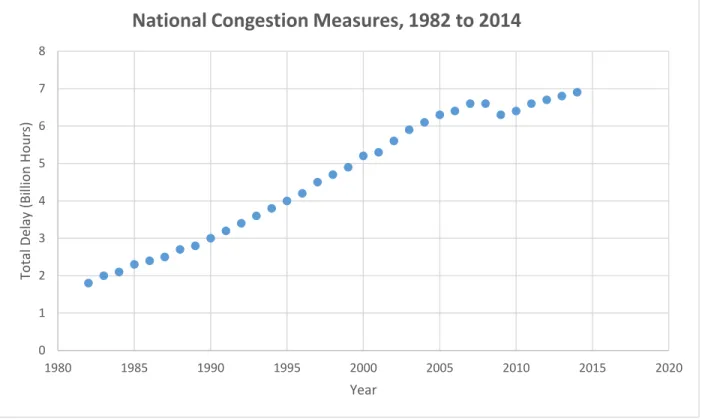
Rapid expansion of cities followed by urban agglomeration has been a very common phenomenon witnessed in the U.S. in recent years. Agglomeration economies have created mega-regions, produced new employment opportunities, and stimulated urban economic development, while attracted more people to cities. As the majority of population of a country is now living in cities, providing sufficient infrastructures for people to live and travel is a daunting task (Edwards and Smith, 2008). The shortage of needed residential, commercial, and transportation infrastructure is further aggravated by improper planning and difficulty of determining employment, population, transportation and infrastructure growth (Duranton and Turner, 2012). Economic outlook and population growth of a city has a profound impact on the development and use of its transportation systems and transportation infrastructure. According to the U.S. Department of Transportation, in 2014, total highway travel was 3,025,656 million vehicle miles or 4,371,706 million passenger miles, which was slightly higher than the previous years in spite of the nationwide economic recession (National Transportation Statistics, 2016). According to the Urban Mobility Report 2015, total national congestion delay has been increased every year (except 2008 and 2009) since 1982 (Schrank et al., 2015). FIGURE 1 shows the trend in national congestion from 1982 to 2014.

(12)

2

FIGURE 1 Trend of national congestion from 1982 to 2014. (Data source: Urban Mobility Scoreboard 2015)

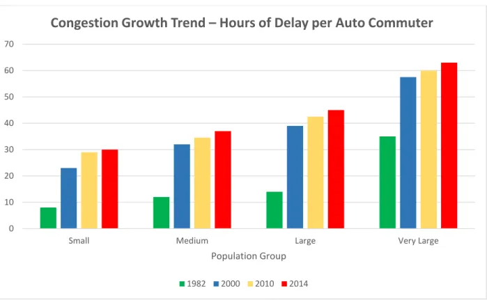
The urban areas can be divided into four groups based on population size, - very large with 3 million and over population, large with 1 million to less than 3 million populations, medium with 500,000 to less than 1 million populations and small with less than 500,000 populations. According to Bureau of Transportation Statistics (BTS), travel time indices were reported to be 1.32, 1.23, 1.18 and 1.14 for these 4 types of urban areas with a congestion cost of 5259, 1281, 474 and 191 million dollars, respectively in year 2014. The Travel Time Index is defined as the ratio of travel time in the peak period to the travel time at free-flow conditions. Therefore, a value of 1.32 indicates that a trip time in the peak hour would be 1.32 times of the free-flow travel time (National Transportation Statistics, 2016). Obviously, the larger the urban areas, greater is the peak hour travel time, as well as the congestion cost. However, congestion is not just a big city problem; it is

0 1 2 3 4 5 6 7 8 1980 1985 1990 1995 2000 2005 2010 2015 2020 To ta l Del ay (B ill ion H o u rs ) Year

(13)

3

worse in areas of every size (Schrank et al., 2015). For different population sized cities, the following figure shows the congestion growth trend in hours of delay per auto commuter:

FIGURE 2 Congestion growth trend in different population sized cities. (Source: Urban Mobility Scoreboard 2015)

Congestion means extra travel time and the uncertainty of travel, which adversely affects the daily routine of travelers. It is important to notify travelers of the probable travel time so that they can choose alternative routes and/or re-schedule their departure times and activities accordingly. Travel time, an important component of Advanced Traveler Information System (ATIS), is a key factor to determine the travel decisions in response to unexpected delays (Khattak et al., 1996). As a part of Intelligent Transport System (ITS), ATIS performs two basic functions, routing and navigation through continuous monitoring of transportation system and evaluation of its performance. Integrated with a traffic data collector- Advanced Transportation Management System (ATMS), ATIS provides information about recurrent and non-recurrent congestions (Qiu

0 10 20 30 40 50 60 70

Small Medium Large Very Large

Population Group

Congestion Growth Trend – Hours of Delay per Auto Commuter

(14)

4

and Cheng, 2007) which benefits individual travelers and a road network as a whole, especially at the time of traffic congestions (Levinson, 2003). Besides the measurement of transportation system performance, travel time has been used to assist to predict travel time and traffic state, which helps the traffic operations room in versatile ways.

In general, ITS integrates advanced communications, control, electronics, and computer hardware and software technologies into the transportation infrastructure and in vehicles (Sussman et al., 2000) and improves surface transportation system performance by using its electronic surveillance, communications, and traffic analysis and control technologies with various sensor technologies- inductive-loop detector, magnetic detector, video image processor, microwave sensor, and infrared sensor (Handbook, 2006). ATIS services include dynamic message signs, dynamic information (e.g. real-time travel times and congestion information), in-vehicle navigation systems and dynamic route guidance to reduce trip uncertainty (Sussman et al., 2000). In ATIS, fixed point traffic sensors, cellular geo-location technologies (Sussman et al., 2000), automatic vehicle identification (AVI) systems (e.g. Bluetooth readers, electronic toll collection tags, license plate readers, and signature re-identification based on detector or magnetometer measurement) are being used to measure and/or estimate the travel time (Xiao et al., 2014). “Automatic vehicle identification (AVI) data allows individual travelers to be time stamped at different parts of the transportation system, enabling the quality of service to be measured by calculating travel times between pairs of points in the system” (Day et al., 2012). Amongst all the available techniques, Bluetooth has emerged as one of the fastest growing data collection technologies whose market share is continuing to rise, mainly due to its cost effectiveness. Bluetooth is a probe based (Puckett and Vickich, 2010) AVI technique for collecting travel time data. Each Bluetooth device contains a unique electronic identifier known as a Media Access

(15)

5

Control (MAC) address. By mounting a simple antenna adjacent to the roadway, MAC addresses of other devices in range can be logged. When a logged MAC address matches at two consecutive stations, the difference in logging time stamps is used to estimate travel times and the corresponding traffic speed (Bachmann et al., 2013). The process of Bluetooth detection is illustrated in FIGURE 3:

FIGURE 3 Process of Bluetooth traffic monitoring (Haghani et al., 2010).

Travel Time and its Estimation: Arrival vs. Departure time based travel time

Travel time is measured by the time elapsed when a traveler moves between two distinct spatial positions (Carrion and Levinson, 2012). Over a decade, various studies have attempted to define travel time estimation (e.g. instantaneous travel time, experienced travel time (Xiao et al., 2014), and predicted travel time (Bhaskar et al., 2011)), but the definitions lack clarity and have created confusion and inconsistency in data collection and analysis (Bhaskar et al., 2011, Toppen and

(16)

6

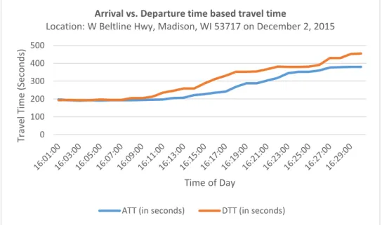
Wunderlich, 2003). Recently, however, one study made clear the distinction between arrival time-based travel time (ATT) and departure time-time-based travel time (DTT) (Kim et al., 2009). ATT and DTT have two different estimation algorithms for real time computation. ATT refers to the travel time associated with arrival at the destination, while DTT refers to the travel time associated with departure from the origin. Hence, a vehicle starting at 8:30am from place A and reaching place B at 9:00am will yield the ATT (𝐴𝑇𝑇_{𝐴𝐵@9:00𝐴𝑀}) and DTT (𝐷𝑇𝑇_{𝐴𝐵@8:30𝐴𝑀}) of link AB at 9:00am and 8:30am, respectively. In practice, ATT and DTT are link-dependent, not vehicle-dependent, as they refer to the link-based travel time. ATT and DTT may available simultaneously if many vehicles travel a link continuously. Practitioners usually treat ATT as the travel time in an ATIS due to the lack of available DTT; however, this reported ATT is one-step (step interval = travel time) earlier than the actual travel time to be experienced (DTT) by drivers. Although ATT and DTT differ slightly in a free-flow condition, the difference can sharply escalate at the onset and end of traffic congestion. FIGURE 4 shows the difference between ATT and DTT from free-flow to onset of congestion for a link of 3.1 mile with a free-flow travel time of 202 seconds.

FIGURE 4 Arrival vs. Departure time based travel time. 0 100 200 300 400 500 Tra ve l T im e (Se con d s) Time of Day

Arrival vs. Departure time based travel time

Location: W Beltline Hwy, Madison, WI 53717 on December 2, 2015

(17)

7

The graph presented above clearly states that the difference between ATT and DTT becomes higher at the onset of congestion. Data show that ATT usually lags behind DTT during a transition of traffic state, and the difference starts to decrease when the traffic state becomes stable. Information on travel time during a transitional state, as opposed to a stable state, is more important to the travelers. Ideally, the travel time in ATIS should be the prediction of travel time experienced by a traveler, or DTT. This predicted travel time also helps ensure proper and proactive operations and management of traffic in a network.

Travel Time Variability and Reliability

The variation of travel time on a route with the same origin and destination can be defined as the travel time variability. According to Arup et al., there are two distinguished components of travel time variability- incident related variability and day-to-day variability (Arup et al., 2004). The former one is random, whereas the latter one is predictable as it is demand and capacity related variability. Travel time variability is reciprocal to the reliability of travel time. According to Carrion and Levinson, higher the variability, lower the reliability, and hence, the unreliability can be defined as the measure of spread of the travel time probability distribution (Carrion and Levinson, 2012).

Outcomes of recurrent congestions are the day-to-day variability of travel time, which is somewhat anticipated by the travelers, specifically, the travelers who travel a specific route regularly. To adjust this anticipatable variation, travelers offset the added cost. The added cost consists of the value of travel time whose variability and reliability has been measured in several studies (Hensher and Truong, 1985, Eliasson, 2004) and was considered in cost-benefit analysis (CBA) of transportation projects (Kouwenhoven et al., 2014). A few studies have been conducted

(18)

8

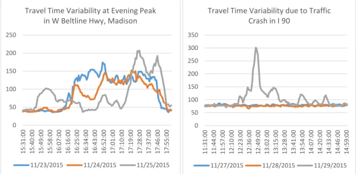
to explore the quantitative methods of forecasting travel time variability (Sohn and Kim, 2009) and the effect of variability reduction (Eliasson, 2006). Travel time variability also includes the unpredictable variations that lead to the uncertainty of travel time. This randomness is the effect of non-recurrent congestions. FIGURE 5 (a) and (b) illustrates the effects of both recurrent and non-recurrent congestions respectively:

(a) (b)

FIGURE 5 a) Predictable (peak hour) b) unpredictable variability in travel time

Unreliable i.e. highly oscillating travel time is undesirable to travelers due to its cost in daily activities. Since it is impossible to remove the variations in travel time completely, informing the travelers in advance can be thought of as a better option. Therefore, at the beginning, the accurate prediction of travel time (DTT) using available real time ATT and then, short term forecasting (if necessary) might be an effective endeavor to ensure better assistance for travelers. However, the accuracy of predicted or forecasted travel time may vary with the variability of travel time. Higher accuracy can be achieved for travel time with lower variability and vice versa. As a

0 50 100 150 200 250 15:31:00 15:40:00 15:49:00 15:58:00 16:07:00 16:16:00 16:25:00 16:34:00 16:43:00 16:52:00 17:01:00 17:10:00 17:19:00 17:28:00 17:37:00 17:46:00 17:55:00 Travel Time Variability at Evening Peak

in W Beltline Hwy, Madison

11/23/2015 11/24/2015 11/25/2015 0 50 100 150 200 250 300 350 11:31:00 11:44:00 11:57:00 12:10:00 12:23:00 12:36:00 12:49:00 13:02:00 13:15:00 13:28:00 13:41:00 13:54:00 14:07:00 14:20:00 14:33:00 14:46:00 14:59:00 Travel Time Variability due to Traffic

Crash in I 90

(19)

9

result, acceptable accuracy range for forecasted travel time should be narrower for the travel time with low variability than the travel time with high variability and vice versa (Toppen and Wunderlich, 2003).

Travel Time Data Collection Technologies

The application of travel time information is mainly two folds - congestion measurement and real-time travel information. According to Turner, electronic distance-measuring instruments (DMIs), computerized and video license plate matching, cellular phone tracking, automatic vehicle identification (AVI), automatic vehicle location (AVL), and video imaging are some advanced techniques of collecting travel time data. Among these, non-expensive electronic DMIs and expensive computerized and video license plate matching are most applicable for congestion measurement and monitoring. Cellular phone tracking, AVI, and AVL systems may require a significant investment in communications infrastructure, but appropriate for real-time information. When an observer records his travel time at predefined checkpoints using a data collection vehicle, it is known as the probe vehicle technique (Turner, 1996).

As a probe based AVI technology, Bluetooth data is not immune to the sampling issue that directly affects the accuracy and reliability of the information it provides. Its sampling rate is very low and depends on many issues including configuration, installation, location etc. Due to the low sampling rate and sampling error, data may not be available for every minutes and a single outlier may affect the travel time sharply. Despite of having some sampling issues, Bluetooth data has several advantages over other data sources including anonymous and continuous data collection. Moreover, Bluetooth data can be used as a Ground Truth data after applying proper data processing algorithm (Haghani et al., 2010). Ideally, a smoothed average travel time of all vehicles traversing

(20)

10

a target link or route is termed as “ground truth” for that link or route due to the variation in traveling speed among different vehicles (Toppen and Wunderlich, 2003).

Research Gaps

For Bluetooth data, sample size depends on the penetration rate of detectable Bluetooth signals in the traffic stream and the total number of vehicles per unit time. Generally speaking, higher sample size usually represents the population better than a lower sample size. The dilemma is that real-time information requires the travel real-time to be updated on a frequent basis, which may contradict with the desire for a large sample size collected over a long period given a low penetration rate. Another problem regarding sample size involves the penetration rate that varies over time. Provided that a valid sample size is determined, the time-varying penetration rate results in a changing time interval for updating the travel time: higher penetration rate requires a shorter time interval for travel time than lower penetration rate and vice versa. Dynamic time interval for travel time update creates confusion to travelers as information should be updated neither too frequent nor too slow. Another undesirable feature is the computation complexity added by constantly finding the proper time period that contains target samples. A few studies have been conducted to address the low sampling challenges of travel time estimation using Bluetooth data, hardly any of these has even mentioned sampling interval.

Bluetooth data is sensitive to the sampling issue that directly influences the accuracy and reliability of the information it provides. As mentioned earlier, its sampling rate is very low and depends on many aspects including configuration, installation, location etc. Despite of having some limitations, Bluetooth Technology (BT) has become popular due to various reasons including low cost. Due to the low sampling rate and sampling error, data may not be available in every

(21)

11

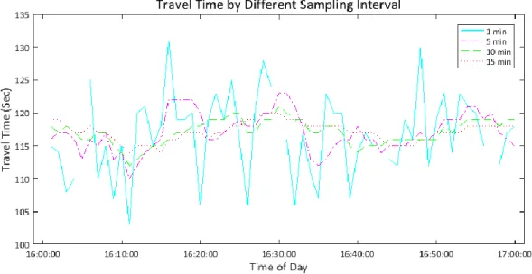
minute and a single outlier may affect the travel time sharply. Accumulation of data in several minutes would help to overcome these limitations. However, accumulation is a trade-off between the real time sensitivity and accuracy of the travel time. Since the longer the aggregation time period is, the more real time essence of travel time is compromised, it is imperative to know about the loss of stochasticity, a predominant property of travel time. FIGURE 6 delineates the loss of this predominant property among different aggregation intervals of travel time:

FIGURE 6 Variation in travel time stochasticity.

According to FIGURE 6, travel time variability decreases and coverage of intervals with no-sample increases in higher aggregation intervals e.g. min, 5-min, 10-min and 15-min. The 1-min sampling interval yields excessive instability in travel time. Therefore, it is imperative to identify the appropriate time interval for sampling Bluetooth data that balance the need for accurate, reliable, and timely update of the travel time on freeways.

Travel time estimation is not a new topic. In general, the travel time in an ATIS is ATT due to the lack of available DTT; however, this reported ATT is one-step (step interval = travel time) earlier than the actual travel time to be experienced (DTT) by drivers, as mentioned earlier.

(22)

12

ATT usually lags behind DTT during a transition of traffic state, and the information on travel time during a transitional state, as opposed to a stable state, is more important to the travelers. Therefore, DTT should be manifested as real time travel time from the viewpoint of travelers. The travel time in ATIS should be the travel time experienced by a traveler, or DTT derived by the prediction from ATT. This predicted travel time also helps ensure proper and proactive operations and management of traffic in a network. Unfortunately, no prediction algorithm has been applied in any study to predict DTT from the available ATT. Moreover, very few studies have distinguished between DTT and ATT or attempted to estimate DTT (Kim et al., 2009).

Research Goal and Objectives

The overarching goal is to develop a comprehensive model for Bluetooth data preparation, accurate travel time estimation considering low sampling issues and thus, short-term travel time prediction on freeways based on the estimated travel time. To attain this research goal, the following objectives are proposed:

Firstly, identifying and recommending an appropriate time interval for sampling Bluetooth data that balance the need for accurate, reliable, and timely update of the travel time on freeways. Rather than determining a fixed sample size that leads to varying time interval for travel time update, a simple method has been proposed considering a balance between real time sensitivity and reliability of the travel time estimation. A framework should be developed to quantify the effect of aggregation on intervals in terms of high confidence sample rate, sample penetration rate and measure of succession.

(23)

13

Secondly, developing a dynamic filtering algorithm to estimate ATT and DTT reliably. This objective requires the development of an efficient computer algorithm to process, refine and integrate massive Bluetooth dataset to calculate the travel time.

Finally, proposing a prediction algorithm that is capable of predicting DTT from ATT accurately. It requires the discerning selection of appropriate method and critical analysis of its prediction performance.

Thesis outline

The remaining part of this thesis is organized as follows:

Chapter 2 explores the literature review on Bluetooth technology, outlier detection procedure, sampling requirements of low sample data, and travel time estimation and prediction.

Chapter 3 discusses about the massive dataset and its preparation. The preparation includes introduction of an appropriate filtering model supported by the principles from the existing dynamic travel time outlier filters. It also demonstrates the performance of proposed filtering model in travel time estimation briefly.

Chapter 4 examines the existing strategies to set sampling unit (sample size or sampling interval) for travel time estimation using Bluetooth data with low sample rates and inaugurates a novel procedure to find the suitable sampling unit.

Chapter 5 introduces travel time prediction model to predict DTT from ATT.

Chapter 6 summarizes the entire research, includes the contributions of the study and concludes the thesis with explanation regarding future research scopes.

(24)

14

CHAPTER II. LITERATURE REVIEW

The probe vehicle techniques, an intelligent transportation system (ITS) application, are primarily designed to collect data in real-time for traffic operations monitoring, incident detection, and route guidance applications including travel time. When driving a probe vehicle, different driving approaches (average, chasing and maximum car) can be followed to record the travel time using manual, DMI (Distance Measuring Instrument) or GPS (Global Positioning System) recorder. A probing technique, has both advantages like wide and flexibility of data collection area and disadvantages like single vehicle representation of entire traffic stream. Alternatively, probe vehicle data can be passively collected through manual or automatic vehicle identification, such as license plates, toll tags, cellular phone or Bluetooth signals. License plate matching techniques include three approaches – a) manual, b) video with manual transcription and c) automatic character recognition. Each approach has its positive and negative aspects. Cellular probe or wireless network data (handoff and location update) also has several pros and cons, which emphasizes the need for careful analysis of the characteristics of a network. Validation and evaluation can be difficult for these types of data due to lack of ground truth. In addition, the use of absolute or relative error is not straightforward to know the performance, because use of absolute error is unjust to high speed cases and relative error is unreasonable for low speed cases (Qiu and Cheng, 2007). After all, automatic vehicle identification (AVI) is the most accurate technique (depending on sufficient market penetration) where vehicles are equipped with transponders or toll tags (Toppen and Wunderlich, 2003).

(25)

15

Review on Bluetooth Technology

Amongst the AVI techniques, market penetration rate of Bluetooth devices is comparatively low. After compared to Automatic License Plate Recognition (ALPR) technology, it was found Bluetooth represented actual conditions very well at a fraction of the price of an ALPR despite of having low sampling rate (Wang et al., 2011). Other studies claim that the technology is powered by the effective matching capability, low cost and above all, sufficient accuracy with a professional setup (Turner et al., 1998, Araghi et al., 2015, Wang et al., 2011).

More studies found that the information collected using Bluetooth technologies could be subject to errors due to low penetration rate, communication range, location placement and installation, and some offered solutions. A study based on a 24 hours empirical data set on I-65 in Indianapolis has found that the MAC address is discoverable for 7.4% of the vehicles within 30′ and 6.6% of the vehicles between 102′ and 114′ (Brennan Jr et al., 2010). The freeway market penetration rate usually varies within a certain range, for instance, 5-11% (Quayle and Koonce, 2010) or 6.25% (Click and Lloyd, 2012) of total volume based on 24 hours counts. Communication range of Bluetooth devices is up to 300 feet, which can be affected by power rating, antenna quality, and obstructions between units etc. (Click and Lloyd, 2012, Bachmann et al., 2013). For instance, vertically polarized antennas with gains between 9dBi and 12dBi are the best antennas for travel time data collection (Porter et al., 2013). Limitations associated to MAC address scanners such as scanning frequency and maximum number of ID capturing in a same time frame can play vital role during data collection (Abedi et al., 2013). Moreover, the optimal number and location of Bluetooth sensors in a network for the reliability of the collected data(Asudegi, 2009) were thoroughly investigated and recommendations were made.

(26)

16

Malinovskiy et al. considered several types of Bluetooth detector antenna, several detector placement locations and Bluetooth device configurations (e.g. lane-length covered, antenna direction, opposite tandem, strength etc.) to estimate Bluetooth based travel time error on a short corridor for a 15-mins window (Malinovskiy et al., 2011). Detection zone, device mounting location, antenna direction and even, combination of mounting locations and antennas have significant impact on accuracy of travel time estimation. Bluetooth data quality related error can be generally classified into - spatial, temporal and sampling error (Malinovskiy et al., 2011, Mei et al., 2012). Spatial error indicates the lack of information about exact position of the vehicle at the time of detection. Temporal error includes multiple detection or no detection at all within the time range of up to 10.24 seconds after it enters the detection zone. Spatial and temporal error jointly lead to the measurement error. Sampling error refers to the low sampling rate that is unable to represent the population. In addition, Malinovskiy et al. considered sampling bias as a type of sampling error. Sampling bias includes error due to fast moving cyclists and bus passengers’ Bluetooth devices, multiple Bluetooth devices in a single vehicle, vehicles with planned en route stops. Algorithms are designed to detect and remove some of the biases since a single outlier may affect the travel time sharply due to low sample rates. Intuitively, accumulation of several minute data would help to minimize the measurement error and a simple and robust outlier-filtering algorithm to overcome the limitation of sampling bias.

Review on Outlier Detection

The prime concern of outlier detection algorithms is to detect extreme travel times that result from sampling bias. Introducing a novel method named overtaking rule, Robinson and Polak filtered out vehicles that took indirect route, stopped en-route, were not restricted to normal traffic

(27)

17

regulations (e.g. emergency vehicles traveled over speed limit), traveled in an unusual fashion (Robinson and Polak, 2006). The percentile tests and deviation tests are other recognized outlier detection algorithms (Liu, 2008). Influenced by these methods, Liu introduced a generic algorithm to work offline. This algorithm needs future data set as well as whole dataset to define its parameters. However, the percentile test is a way to filter out outliers based on predefined percentile range (lower and upper limit). Therefore, the application of this method is subject to having prior knowledge of travel time distribution. In a deviation test, the range is defined by a critical distance (CD) from the median of the travel times within each period. Clark et al. applied percentile, deviation and traditional (modified) z- or t-statistical test (Clark et al., 2002). Traditional z- or t-statistical test outperformed other two methods, specially, in the presence of incident condition.

Fixed range outlier filtering methods are not suitable for travel time filtering due to local travel time turbulences, specially, at onset and end of congestion. Instead of imposing arbitrary bound, data driven real time adaptive bound (Dion and Rakha, 2006), moving average speed based lower and upper bound (Haghani et al., 2010) have been introduced by researchers in different adaptive algorithms. Compared to conventional algorithms, Dion and Rakha incorporated few simple but significant alterations in their proposed adaptive method. The main alteration includes the expansion of data validity window when three consecutive observations fall either above or below (same side) the validity window. Although this key adjustment helps to capture sudden changes in travel time trend, it is prone to the inclusion of extreme outliers. As a result, accuracy of travel time estimation would be compromised. Based on the algorithm proposed by Dion and Rakha, Moghaddam and Hellinga proposed a proactive method using pattern recognition model which showed superior performance (Moghaddam and Hellinga, 2014a). All these adaptive

(28)

18

methods are associated with some degree of complexity due to real time (online) applicability. For offline processing of dataset, a simplified version of the algorithm proposed by Dion & Rakha or Lie should be adequate to serve the purpose if applied appropriately.

Review on Sampling Techniques (Rate or Interval)

Sample size not only varies with the techniques of data collection but also varies with the types of studies or application. In a typical travel time study, sample size could be fixed by the researcher prior to data collection (Turner et al., 1998). In contrast, continuous samples are necessary for a real time application like travel time prediction.

Bluetooth technology has the advantage of collecting data continuously and anonymously (Moghaddam and Hellinga, 2014b). Different studies reflect researchers’ efforts to find sampling requirement, more specifically, sample size for probe vehicles (Turner and Holdener, 1995, Chen and Chien, 2000, Li et al., 2005). Chen and Chien estimated the minimum sample size using statistical method and applied heuristic approach using CORSIM simulation to find the minimum number of required probe vehicle with a desired statistical accuracy. Their study suggests that 3-12 probe vehicles are required for each 5-min interval depending on traffic flow rate from low or high to moderate. Similar method based approaches have also been applied to define the minimum sample size considering cost, measurement error, true error and confident interval (Toppen and Wunderlich, 2003). Li et al. utilized Chris’s probe vehicle sampling size model combining capacity constraints of wireless communication system (Li et al., 2005). The Chris’s model (Ygnace and Drane, 2001) utilizes the information of traffic density, average link length and fraction of vehicles sampled to get the coverage. Ygnace and Drane studied cellular phones as probe vehicles to find the probe vehicle size to estimate travel time with 5% accuracy (Ygnace and Drane, 2001). In

(29)

19

addition, Jiang et al. studied the impact of probe vehicle sample size and sampling interval and concluded that the time interval had little effect for same sample size. They also demonstrated that the estimation error of average link travel time varied steadily when the sample size reached at a certain threshold (Jiang et al., 2006). Therefore, the accumulation of several minute samples are capable to provide reasonably reliable travel time regardless of population size. In a study, Click and Lloyd concluded that the intervals with sample size 8 or more possess higher confidence in Bluetooth data on rural freeways (Click and Lloyd, 2012). More accuracy can be ensured by applying appropriate methods of estimation. Araghi et al. estimated travel time in four different approaches- min, max, median and average travel time within two different sample intervals (15 and 30 mins) and found the min and median travel time were more robust in the presence of outliers (Araghi et al., 2015).

Although, studies regarding the impact of sampling interval and sample size are unavailable about Bluetooth data, studies related to probe vehicle explicitly exhibit that the sampling interval and sample size are interrelated. Therefore, a generic interval would not be effective for any dataset since sample size within an interval is uncontrollable. Sometimes, low sampling rate affects the minute-by-minute data availability. Nevertheless, accumulation of several minute data would increase number of samples within a certain time interval without affecting the penetration rate. Since accumulation of data is a trade-off between the real time sensitivity and accuracy of the travel time, fixing the accumulation time window i.e. sampling interval is excessively challenging. A data driven approach would be appropriate to decide the interval, ensuring minimum error in estimation of travel time.

(30)

20

Review on Travel Time Estimation

In transportation science, travel time, the time to traverse a specific route, can be differentiated in accordance with its measurement procedure. When a travel time is deduced from a spot based measurement (e.g. spot speed), it is known as instantaneous travel time. Contrary, an experienced travel time is a travel time that a traveler actually experienced; which is measured based on the start and end time of a journey. This experienced travel time considers traffic states and hence, it is the measure of free flow travel time and additional travel time (at no free flow state of traffic) due to the variability in traffic state. Measuring the experienced travel time is excessively simple for individual travelers but estimation based on samples to reflect the expected value of the actual travel time can be complicated due to several contributing factors.

As already discussed, Bluetooth is a relatively new technology that has become popular due to several reasons including low cost and anonymous detection of vehicles as well as travelers who carry Bluetooth devices accessible through designated roadside Bluetooth stations. Due to the technical complexity and limitations, none of the data collection procedure for travel time estimation including Bluetooth is error free. Consequently, collected data contains error that emerges the need for exploration of different robust techniques. In response, researchers introduced several outlier-filtering techniques (as studied earlier in this literature) to remove various types of error from the data. Once data is cleaned, it can be used to estimate experienced travel time using simple average method. Travel time data is available from those vehicles or travelers who have already traversed the route. Hence, the estimated travel time provides the most recent historic or current travel time as a real time travel time.

Since the most recently experienced travel time is the key to predict the future travel time, many studies have been conducted to ensure accurate estimation of travel time in a real time

(31)

21

fashion (Dion and Rakha, 2006, Skabardonis and Geroliminis, 2005, Li and McDonald, 2002, Lu and Chang, 2012, Sumalee et al., 2013, Moghaddam and Hellinga, 2014a). Those studies are diversified in terms of data, method and applicability. For instance, (Lu and Chang, 2012) and (Skabardonis and Geroliminis, 2005) applied traffic flow theory based model (queue and delay) to estimate travel time distribution in a signalized arterial using license plate recognition system data, and loop detector data respectively. (Moghaddam and Hellinga, 2014a), and (Dion and Rakha, 2006) detected outliers, removed and took simple average to estimate travel time for arterial, and freeway using Bluetooth, and AVI respectively. At the same time, researchers have also been involved in prediction of travel time as a sequential research of travel time estimation. As discussed in earlier chapter, DTT (will be experienced travel time) is more appropriate to be manifested as real time travel time rather than ATT (the most recently experienced travel time) from the viewpoint of travelers. Unfortunately, no research except (Kim et al., 2009) has been conducted to predict DTT from ATT. Although there is a research gap from the viewpoint of research goal and objectives, this topic has been over saturated in terms of, different methodologies resulted from a plenty of studies conducted over a decade.

Broadly, travel time prediction methods can be classified into two categories: the classical approach (Oda, 1990) which includes statistical (Rice and Van Zwet, 2004) and time series models (Al-Deek et al., 1998, Hamed et al., 1995), and the data-driven approach (Vlahogianni et al., 2014, Zheng and Van Zuylen, 2013, Zhang et al., 2014, Wu et al., 2004, Myung et al., 2011). Integration of different models, for example, a time-series model - auto regressive integrated moving average (ARIMA) with an embedded adaptive Kalman filter, has also been applied to develop a multistep travel time predictor (Xia et al., 2011). Due to the instability of traffic states, most classical approaches have shown to be incapable of better prediction, especially with regard to structured

(32)

22

and unstructured data (Vlahogianni et al., 2014). Since data-driven approaches fit easily with massive datasets, researchers have applied neural and Bayesian networks (Zheng and Van Zuylen, 2013, Oh and Park, 2011, Li and Rose, 2011, van Hinsbergen et al., 2009, Fei et al., 2011, Van Lint et al., 2005), fuzzy and evolutionary techniques (Zhang et al., 2014), support vector regression (Wu et al., 2004, Vanajakshi and Rilett, 2007), and k-nearest neighbor (Myung et al., 2011, Bustillos and Chiu, 2011) model to directly or indirectly predict travel time. Rather than using as a black-box or location-specific model, Van Lint et al. proposed for the state space neural network based on the lay-out of the freeway stretch of interest (Van Lint et al., 2005). However, according to Myung et al., the use of non-representative samples to train artificial neural-network (ANN) model may lead to the non-negligible error in prediction since this data driven approach needs to be trained using historical dataset (Myung et al., 2011). In addition, ANN is long training dependent using large historical dataset and non-transferable. Similarly, Support vector regression (SVM), a time-series forecasting format of support vector machine, also needs to be trained by a massive representative dataset.

Researchers have also applied the combination of several data driven techniques to achieve better performance. Li and Chen applied K-mean clustering to partition the dataset, CART-based classification to identify important variables and finally, neural network based approach to predict travel time in freeway with non-recurrent congestion (Li and Chen, 2014). Based on the variable selection method, they selected six scenarios and compared them in terms of mean absolute percentage error (MAPE); and found error rate of 6%-9%. Zou et al. applied MAPE, mean absolute error (MAE) and root mean square error (RMSE) as performance indexes to make a comparison among the output from auto regressive model (AR), vector auto regressive model (VAR), space-time diurnal truncated normal model (ST-D TN) and space-space-time diurnal lognormal model (ST-D

(33)

23

LN) (Zou et al., 2014). This probabilistic prediction method was able to provide the prediction related confidence intervals that reflected the level of uncertainty. Results showed that ST-D LN model performed better in case of predicting multiple time-steps ahead into the future.

One notable observation is that the vector auto regressive model has performed slightly better than other methods in case of 5-min ahead prediction. Unlike the neural networks and some hybrid methods that lack a good interpretation of the model due to the ‘‘black box’’ approach, this model has used theoretically interpretable travel time features (temporal and spatial correlation, diurnal pattern, and the non-negativity of the travel time). Temporal and spatial correlation feature has incorporated information from upstream and downstream locations (similar to vector auto regressive model) into the prediction model unlike the on-site predictor type univariate auto-regressive model. Although the application of diurnal pattern made the model robust in terms of interpretability, it might deteriorate the model performance with the change in pattern due to non-recurrent congestion.

To predict dynamic travel times, Elhenawy et al. proposed a simple and computationally efficient genetic programming algorithm that did not suffer from non-interpretability (Elhenawy et al., 2014). Nevertheless, data requirements to train the model would be specific to the roadway and traffic conditions. Moreover, the minimum data requirement is yet to be investigated.

Usually, performance deteriorates in case of multi-step prediction using the ANN method (Boné and Crucianu, 2002, Parlos et al., 2000). Even after introducing a noble method named time-delayed state-space neural network, Zeng and Zhang has found more than doubled error in the fifth step compared to the first step (Zeng and Zhang, 2013). Hence, Chen and Rakha applied particle filter, a sequential Monte Carlo method, which outperformed other methods including K-NN and Kalman filter (KF) in case of multi-step prediction (Chen and Rakha, 2014b). Their results showed

(34)

24

consistency in systematic error propagation whereas performances of different methods were somewhat reasonably close at only the beginning. The authors also introduced another recursive probabilistic method namely agent based modeling, which is a weighted average of prediction from different agents i.e. predictors generated by the model (Chen and Rakha, 2014a). Each agent used pattern recognition technique to predict the travel time. The concept is somewhat similar to Boosting technique (Schapire, 2003) of machine learning, a concept of combining rough and moderately inaccurate rules so that the combination can produce an accurate prediction rule. A method comparison showed that this agent based model performed better than historic average, instantaneous and k-NN (Chen and Rakha, 2015).

KF has been widely used with different modification (e.g. adaptive KF (Guo et al., 2014) and extended KF (Liu et al., 2006)) in different studies including travel time prediction (Chien and Kuchipudi, 2003, Nanthawichit et al., 2003, Yang, 2005, Chen and Chien, 2001). KF, an optimal recursive data processing algorithm, incorporates all information that can be provided to it and process all available measurements to estimate current value of the variables of interest (Maybeck, 1990). By definition, it can be inferred that KF has two part- process (also known as system or state space) and measurement (also known as observation). Hence, the algorithm includes process update (also known as time update) and measurement update steps. Both the noises related to process and observation have to be white Gaussian.

Nanthawichit et al. formed their state space equation by declaring traffic density and space mean speed as state variables and observation equation by declaring traffic volumes and spot speeds as observation variables (Nanthawichit et al., 2003). Chen and Chien directly used travel time as their input variable in both state and measurement equations. Previous step travel time was multiplied by a transition matrix to obtain the state update equation (Chen and Chien, 2001).

(35)

25

similar studies were conducted using field data (Chien and Kuchipudi, 2003) rather than simulated data (Chen and Chien, 2001). Despite of showing promising results, the studies deficit in some degree of details about the case study including sources of process and measurement (variables’) values. Although only Yang discussed about the effect of noise variance on prediction error, he did not mention about its variability with time-step (equations in article showed that the noise variances were time varying). In addition, no one discussed about the assumed or derived (including the rationale) values of error covariance that have greater effect on prediction performance in case of single step prediction. Regardless of methodologies, single step prediction provides somewhat similar output (as already mentioned) in most comparisons. Therefore, it is expected that the KF, applied with accurate assumptions, would provide reasonable performance in case of predicting travel time.

Moreover, KF can be indexed as a data induced statistical time series based noise-filtering technique. It requires a measurement update, to perform time update i.e. to predict the future step. Hence, the enough knowledge about the process, availability of measurement and reasonable assumptions regarding noise covariance are highly desirable to experience better performance. Moreover, KF provides the way to update the state space when new observations become available; and state space form is the key to handle structural time series models that are nothing more than regression models (Harvey, 1990). Therefore, KF has the robust power to apply with a regression driven time series model. Favorably, KF algorithm exactly matches with the concept of predicting departure time based travel time (DTT) from arrival time based travel time (ATT).

The knowledge regarding the KF noise is intuitively related to the instability in traffic conditions. As mentioned in previous chapter, different types of congestions: recurrent and non-recurrent are responsible for the instability in traffic conditions. The most unpredictable

(36)

26

congestions are the incident related congestions which are known as non-recurrent congestion (NRC).The congestions that exhibit a daily pattern during peak and off-peak periods are known as recurrent congestion (RC) (Anbaroglu et al., 2014). RC is somewhat predictable by travelers. Although NRC combined with RC makes the situation worsen, in some cases, researchers have showed great deal of success in detection, sometimes, distinction of RC and NRC (Hawas, 2007, Dowling et al., 2004, Skabardonis et al., 2003, Garib et al., 1997, Lin and Daganzo, 1997, Ritchie and Cheu, 1993). Accurate distinction is imperative to classify the KF noise related to different traffic state which may lead to the precise prediction of travel time.

(37)

27

CHAPTER III. DATA PREPARATION AND REDUCTION

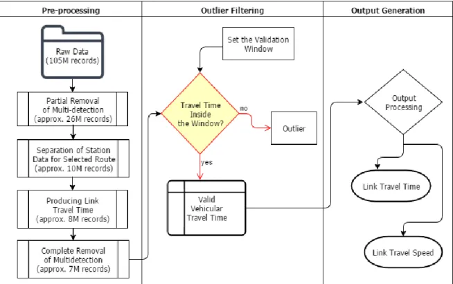
Bluetooth data contains three variables: the MAC ID of the detector, MAC IDs of the detected devices, and the detection timestamp. In spite of a simple data format, a complex processing algorithm is required to produce the final dataset from the source, which stores the entire network data in a single table. For a logged MAC ID, recorded timestamps at two consecutive stations are processed to estimate travel time and the corresponding traffic speed. The complete processing algorithm can be subdivided into three major parts: a) data pre-processing, b) outlier filtering, and c) output generation. The detailed description of the processing algorithm is included below with a brief description of the data characteristics.

Data Description

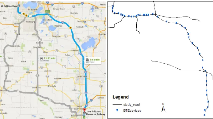
The selected study area consists of a 62.8-mile long route, or approximately 47.5 miles on I-90 and the remaining on the Beltline Highway in Madison, Wisconsin. The route is equipped with 41 unequally spaced Bluetooth stations, resulting in 40 links. The first 21 links are on I-90, the 22nd link is on both corridors, and the remaining links are on the Beltline. The spacing varies from 1.3-3.4 miles on I-90 and 0.4-1.3 miles on the Beltline Highway. FIGURE 7 shows the study area and the stations’ locations.

(38)

28

FIGURE 7 Study Area (Wisconsin, US) with the location of Bluetooth Devices/Stations.

Forty-seven days’ worth of data (11/16/2015-01/01/2016) containing more than 100 million records was collected from traffic in both directions. Half of the records were from outside the study-area. Each station of the one hundred stations selected captured around one million records for 47 days, or 67,680 minutes. However, a large portion (approx. three-fourths) of the data are either corrupted or contaminated due to multiple detections and unsuccessful detections (i.e. not detected in two consecutive stations). Therefore, the average penetration rate would be roughly 3-4 samples per minute. Extensive efforts have been assumed to ensure the data quality.

Data Processing

Efficient and reasonable data processing was made possible by automation. Initially, data was queried from an Oracle database to remove unnecessary records like multiple detections, reducing the records to a reasonable number. Then, a Java application has been developed to further process

(39)

29

the previously filtered dataset. FIGURE 8 shows the complete procedure of data processing followed by the detail descriptions in following sections.

FIGURE 8 Data processing procedures

Pre-Processing

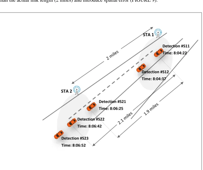
The primary goal of data pre-processing is to clean unnecessary records and prepare a smoothly workable dataset containing calculated travel time of each vehicle. A Bluetooth station usually detects a Bluetooth device in its range more than once. The number of such detections can increase significantly due to planned or unplanned stopping of vehicles. A general inspection of the dataset revealed that such detections usually vary two to four times. Detecting a vehicle at the end of a station and at the beginning of its upstream station would yield maximum spatial error. Since the study data lack of signal strength information, the record of first detection has been preserved carefully to minimize such error. If signal strength information were available, the strongest signal

(40)

30

(of each multi-detection) data would have been preserved to estimate the travel time. Since the detection is automatic, it is impossible to ensure a vehicle’s detection at the points having same signal strength in different detection zones. Consequently, it is impossible to avoid spatial error of detection, even by using the strongest signal information. For instance, the strongest (among all detections) signals at S11 and S22 points (assumed) could provide the longer length (2.1 miles) than the actual link length (2 miles) and introduce spatial error (FIGURE 9).

FIGURE 9 Detections of a vehicle at two consecutive Bluetooth stations.

In addition, first detections (at S11 and S21 points) may provide the shorter length (1.9 miles) than the actual link length (2 miles) and also introduce spatial error. Either way it may contain spatial error. Oracle queries helped clean up the multi-detection (records except the first one were

Detection #S11 Time: 8:04:22 Detection #S12 Time: 8:04:37 Detection #S21 Time: 8:06:25 Detection #S23 Time: 8:06:52 Detection #S22 Time: 8:06:42 STA 1 STA 2

(41)

31

deleted), resulting in the total number of records decreasing from 105 million to 26 million. The data was then separated by each station for the selected routes, further reducing the records to 10 million. When travel time of each vehicle was estimated from the separated station data, unsuccessful detections were automatically ignored due to the vehicle’s detection timestamps from two adjacent stations. Next, the reduced dataset of 8 million samples was processed through a robust Java-based pre-processing module that investigated each record individually and cleaned all unnecessary records based on the following principle:

A vehicle cannot be detected twice in a station, 𝑆𝑇𝐴1 without being detected at least once in its upstream station, 𝑆𝑇𝐴2 within the time gap of two detections in 𝑆𝑇𝐴1. If so, these are redundant detections for any single trip.

For example, a vehicle detected on 08:59am, 09:01am and 09:08am at 𝑆𝑇𝐴₁, and on 09:04am at 𝑆𝑇𝐴2. Detection on 09:01am is redundant since there is no detection at upstream station 𝑆𝑇𝐴2 in between 08:59am and 09:01am. In addition, none of the detections on 09:01am or 09:08am is a redundant detection since there is a detection at upstream station 𝑆𝑇𝐴₂ on 09:04am. The pre-processed dataset of 7 million records containing the journey start time, end time and travel time of each vehicle was further processed to filter outliers.

Outlier Filtering

Outlier filtering is a challenging task due to the possibility of treating a good sample as an outlier. Various studies have been conducted previously to define and filter outliers, and a wide range of methods, simple to complex, have been introduced. In this study, a simple yet robust statistical approach has been applied in which the key of filtering outlier or selecting good samples is to define the validation window i.e. the upper and lower boundary (of travel times). The lower

(42)

32

boundary can be defined based on the assumption that a vehicle’s speed cannot exceed more than the double of a posted speed limit, or it is an outlier

𝑡𝑡𝑙𝑜𝑤𝑟 = 𝑡𝑡𝑓𝑓

2

⁄ (3.1)

Where, 𝑡𝑡_{𝑙𝑜𝑤𝑟} and 𝑡𝑡_𝑓𝑓 are lower bound and free flow travel time respectively.

Once the lower boundary is fixed, upper boundary should be dynamically defined by the samples (travel time) because of the inherent stochastic nature of travel time. A dynamic validation window works best in case of outlier filtering (Dion and Rakha, 2006) but the implementation is very challenging due to the unprecedented variability of travel time. Thus, the following equation is proposed:

𝑡𝑡_{𝑢𝑝𝑝𝑟} = 𝑡𝑡_𝑒+ 𝑛. 𝜎_𝑒 (3.2)

Where 𝑡𝑡_{𝑢𝑝𝑝𝑟}, 𝑡𝑡_𝑒and 𝜎_𝑒 are upper bound, expected travel time and expected standard deviation of travel time (samples) respectively. 𝑛 = 1, 2, 3, ….= nth standard deviation.

The expected travel time 𝑡𝑡𝑒 is the predicted DTT and 𝜎𝑒 is the predicted standard deviation of DTT since the actual DTT is unavailable in real time. However, DTT and its standard deviation have been used as 𝑡𝑡_𝑒𝑎𝑛𝑑 𝜎_𝑒 respectively, since the outlier filtering has been accomplished in offline. The unfiltered dataset was processed dynamically using time varying validation window. The time varying standard deviation 𝜎_𝑒 was estimated using the samples from the latest 30mins data and n was set to 2. The decision for sampling previous 30 minutes with n equals to two was made from trial and error for better performance. It is assumed that the standard deviation of the upcoming samples remains similar to the estimated standard deviation of the recently observed samples for a shorter time period. Following figure shows the performance of this simple method:

(43)

33

FIGURE 10 Performance of filtering algorithm during morning and evening peak hours.

Output Generation

Finally, a Java-based programming module produced the travel time and speed data using the outlier-filtered data. Since travel direction is pertinent to travel time, this study used northbound data. 0 500 1000 1500 2000 6:00:00 6:28:48 6:57:36 7:26:24 7:55:12 8:24:00 Tr av el T im e ( Se co nd s) Observations in I-90

Valid Observations Outliers

0 200 400 600 800 1000 15:50:24 16:19:12 16:48:00 17:16:48 17:45:36 18:14:24 Tr av el T im e ( Se co nd s)

Observations in Beltline Hwy

(44)

34

CHAPTER IV. IDENTIFYING SAMPLING INTERVAL

Methodology

The methodology section details the process of estimating travel time by aggregating samples from several minutes and the method for selecting sampling interval.

Travel Time Aggregation

Estimating travel time in one-minute interval is straightforward, like taking the average of available samples. For an interval of more than one minute, two types of aggregation can be considered: a) simple average and b) moving average. The basic difference between these two estimation procedure is that the former one gives a single travel time for the aggregation interval which means same travel time for every minute within the interval while the latter one updates travel time at each minute regardless of interval size. The estimation process is shown in TABLE 1.

TABLE 1 Travel Time Aggregation Process Time of Day 09:01 09:02 09:03 09:04 09:05 09:06 09:07 09:08 09:09 09:10 Travel Times of Samples 𝑡11, 𝑡12 𝑡21 𝑡31, 𝑡32 𝑡41 𝑡51 𝑡61, 𝑡62, 𝑡63 𝑡81 𝑡91 𝑡101 Simple Average N/A 𝑡11+ 𝑡12+ 𝑡21+ 𝑡31+ 𝑡32+ 𝑡41+ 𝑡51 7 Moving

Average N/A N/A N/A N/A N/A 𝑇09:06 𝑇09:07 𝑇09:08 𝑇09:09 𝑇09:10

𝑇09:06= 𝑡₁₁+𝑡₁₂+𝑡₂₁+𝑡₃₁+𝑡₃₂+𝑡₄₁+𝑡₅₁ 7 , 𝑇09:07= 𝑡₂₁+𝑡₃₁+𝑡₃₂+𝑡₄₁+𝑡₅₁+𝑡₆₁+𝑡₆₂+𝑡₆₃ 8 , 𝑇09:08= 𝑡31+𝑡32+ … +𝑡63 7 , 𝑇09:09= 𝑡41+𝑡51+ … +𝑡81 6 , 𝑇09:10= 𝑡51+𝑡61+ … +𝑡91 6

(45)

35 Sampling Interval Selection

The accurate prediction of travel time is mostly constrained by the turbulence in traffic state. No algorithm is able to completely handle the randomness of traffic state i.e. travel time. As a result, researchers use average travel time over the longer time period (usually 15 minutes) to limit the erratic nature of travel time within a tangible proximity. The longer the time period is; the more real time essence of travel time is compromised. Compared to non-aggregated real time data, aggregated data may show better prediction accuracy that is not necessarily the best approximation of the real situation. Therefore, it is imperative to know the measure of succession (of stochasticity, a predominant property of travel time).

Selection of sampling interval is a two-step process: In the first step, the high confidence sample rate for all the sampling intervals will be determined. The high confidence sample rate refers to the percentage of intervals that contain sample sizes equal or more than a predefined required sample size. Then, the sample penetration rate will also be estimated for all the sampling intervals. The sample penetration rate refers to the percentage of intervals that contain at least one sample. Based on the high confidence sample rate and the sample penetration rate, a minimum sampling interval selection would be determined. In the second step, a sampling interval from a bunch of candidate intervals (e.g. 5-min, 10-min etc.) would be selected based on the measure of succession. The candidate intervals must be equal or higher than the selected minimum interval. To measure the succession, a simple but effective method based on travel time reliability measure has been applied.

(46)

36

High Confidence Sample Rate

The high confidence sample rate (𝑅_𝐻𝐶) is the percentage of intervals that contain samples more than a predefined threshold. 𝑅_𝐻𝐶 for a route can be expressed by,

𝑅_𝐻𝐶 =∑ 𝑁𝑛 𝐻𝐶.𝑖

𝑛𝑁 (4.1)

where 𝑁_{𝐻𝐶.𝑖}= total number of high confidence sample interval in a link 𝑖, n = number of links and N = total number of intervals within the analysis period.

Total number of high confidence intervals (𝑁_𝐻𝐶) for a link can be estimated by,

𝑁_𝐻𝐶 = ∑ 𝐼_𝑁 _{𝑗(𝑚/𝑟)} (4.2)

where 𝐼𝑗(𝑚/𝑟) is a Boolean function to determine whether the 𝑗𝑡ℎ interval with m samples has high or low confidence given required minimum sample size, r.

The Boolean function,

𝐼𝑗(𝑚/𝑟) = {1, 𝑚 ≥ 𝑟_{0, 𝑜𝑡ℎ𝑒𝑟𝑤𝑖𝑠𝑒} (4.3)

where m represents number of samples in 𝑗𝑡ℎ interval and r is the required minimum samples.

Sample Penetration Rate

Since the sample penetration rate refers to the percentage of intervals that contain at least one sample, it can be estimated by following the same method of estimating high confidence sample rate using r=0.