Politecnico di Torino
Porto Institutional Repository
[Proceeding] A Comparative Analysis of Software Reliability Growth Models
using defects data of Closed and Open Source Software
Original Citation:
Ullah N.; Morisio M; Vetro’.A. (2013).
A Comparative Analysis of Software Reliability Growth Models
using defects data of Closed and Open Source Software.
In: 35TH ANNUAL IEEE SOFTWARE
ENGINEERING WORKSHOP, HERACLION, CRETE, GREECE, 12-13 OCTOBER 2012. pp.
187-192
Availability:
This version is available at :
http://porto.polito.it/2502526/
since: September 2012
Publisher:
IEEE
Published version:
DOI:
10.1109/SEW.2012.26
Terms of use:
This article is made available under terms and conditions applicable to Open Access Policy Article
("Public - All rights reserved") , as described at
http://porto.polito.it/terms_and_conditions.
html
Porto, the institutional repository of the Politecnico di Torino, is provided by the University Library
and the IT-Services. The aim is to enable open access to all the world. Please
share with us
how
this access benefits you. Your story matters.
A Comparative Analysis of Software Reliability Growth Models
using defects data of Closed and Open Source Software
Najeeb Ullah, Maurizio Morisio, Antonio Vetro’
Control and Computer Engineering Department, Politecnico Di Torino 10129, Torino, Italy
[email protected], [email protected], [email protected]
Abstract— The purpose of this study is to compare the fitting (goodness of fit) and prediction capability of eight Software Reliability Growth Models (SRGM) using fifty different failure Data sets. These data sets contain defect data collected from system test phase, operational phase (field defects) and Open Source Software (OSS) projects. The failure data are modelled by eight SRGM (Musa Okumoto, Inflection S-Shaped, Goel Okumoto, Delayed S-Shaped, Logistic, Gompertz, Yamada Exponential, and Generalized Goel Model). These models are chosen due to their prevalence among many software reliability models.
The results can be summarized as follows
Fitting capability: Musa Okumoto fits all data sets, but all models fit all the OSS datasets
Prediction capability: Musa Okumoto, Inflection S-Shaped and Goel Okumoto are the best predictors for industrial data sets, Gompertz and Yamada are the best predictors for OSS data sets
Fitting and prediction capability: Musa Okumoto and Inflection are the best performers on industrial datasets. However this happens only on slightly more than 50% of the datasets. Gompertz and Inflection are the best performers for all OSS datasets.
Keywords
—
Software Reliability Growth Models, SRGM, Open Source Software, Failure Data, Software Reliability ModelsI. INTRODUCTION
Software development is a brain intensive activity. Therefore, the quality of the product is subject to large variations. Reliability is one of the most important attributes of software quality, which is defined as the probability of failure-free software operation for a specified period of time in a specified environment [47]. Starting from the 70’s different Software Reliability Models (SRM) have been proposed for software reliability characterization and prediction. SRM is a mathematical expression that specifies the general form of the software failure process as a function of factors such as fault introduction, fault removal, and the operational environment [47]. SRM is composed of different parameters. Parameter is a variable or arbitrary constant appearing in a mathematical expression, each value of which restricts or determines the specific form of the expression. The failure rate (failures per unit time) of a software system is generally decreasing due to fault identification and removal. Software Reliability
modelling is done to estimate the form of the curve of the failure rate by statistically estimating the parameters associated with the selected model. The purpose of this measure is twofold: 1) to estimate the extra execution time during test required to meet a specified reliability objective and 2) to identify the expected reliability of the software when the product is released.
In general SRM are categorized as white box and black box. White box approaches analyze the structure i.e. the architecture of the software that has been specified and designed. These models predict the reliability of software on the basis of the relationship among different components and their interactions. These approaches are also called deterministic approaches. They are based on logical complexity, decision point, program length, operands and operators of software. Path-Based Models and State-Based Models are two examples of this type of reliability model. In the literature these models are known as Architecture Based Reliability Models.
Black box approaches treat the software as an entity and ignore the interdependencies of the software internal components. There are some basic assumptions which are similar for all these kinds of models [49].
1. When a fault is detected it is removed immediately. 2. A fault is corrected instantaneously without
introducing new fault into the software.
3. The software is operated in a similar manner as that in which reliability predictions are to be made. 4. Every fault has the same chance of being encountered within a severity class as any other fault in that class.
5. The failures, when the faults are detected, are independent.
The Black Box approaches are classified into different types, Early Prediction Models, SRGM, Input Domain Based Model, and Hybrid Black Box Models. Our work is focused on SRGM models because of their widespread use. SRGM can be applied to guide the test board in their decision of whether to stop or continue the testing. Herein we present a comparative analysis of SRGM models in term of goodness-of-fit, prediction accuracy and correctness based on thirty eight failure data sets containing system test failures data, field and OSS defects data.
The rest of the paper is organized as follows. Section 2 contains background information and literature review. Section 3 provides the goals and research questions of this study; section 4 describes models and data selection. Section 5 describes results; section 6 contains discussion and in 7 threats to validity has been discussed. Section 8 concludes the study.
II. BACKGROUND
A. Reliability Modelling
Software Reliability Models (SRM) can both assess and predict reliability. In reliability assessment SRM are fitted to the collected failure data using statistical techniques (e.g. Linear Regression, Non Linear regression) based on the nature of collected data. In reliability prediction, the total number of expected future failures is forecasted on the basis of fitted SRM. Both assessment and prediction need good data, which implies accuracy - i.e., data is accurately recorded at the time the failures occurred- and pertinence - i.e., data relates to an environment that resembles to the environment for which the forecast is performed-. For reliability modelling, software systems are tested in an environment that resembles to the operational environment. When a failure (i.e., an unexpected and incorrect behaviour of the system) occurs during testing, it is counted with a time tag. Cumulative failures are counted with corresponding cumulative time: when 60% of tests are completed then SRM is fitted to the collected data and used to predict the total number of expected defects in the software [42].
Hence, typically reliability modelling is composed of 5 steps: keeping a log of past failures, plotting the failures, determining a curve (i.e. Model) that best fits the observations, measuring how accurate the curve model is and then using the best fitted model predicting the future reliability in terms of predicting total number of expected defects in the software system.
However, there is no universally applicable reliability model due to the fact that reliability is not independent of the application. One option to select a good model is to fit several models to observed data and take the one that best fits the data. B. Software Reliability Growth Models
SRGM is one of the prominent classes of black box SRM. They assume that reliability grows after a defect has been detected and fixed. SRGM can be applied to guide the test board in their decision of whether to stop or continue the testing. These models are grouped into concave and S-Shaped models on the basis of assumption about failure occurrence
pattern. The S-Shaped models assume that the occurrence pattern of cumulative number of failures is S-Shaped: initially the testers are not familiar with the product, then they become more familiar and hence there is a slow increase in fault removing. As the testers’ skills improve the rate of uncovering defects increases quickly and then levels off as the residual errors become more difficult to remove. In the concave shaped models the increase in failure intensity reaches a peak before a decrease in failure pattern is observed. Therefore the concave models indicate that the failure intensity is expected to decrease exponentially after a pick was reached.
Software Reliability Growth Models measure and model the failure process itself. Because of this, they include a time component, which is characteristically based on recording times ti of successive failures i (i ≥1). Time may be recorded
as execution time or calendar time. These models focus on the failure history of software. The failure history is affected by a number of factors, including the environment within which the software is executed and how it is executed. A general assumption of these models is that software must be executed according to its operational profile; that is, test inputs are selected according to the probability of their occurrence during actual operation of the software in a given environment [8]. There are many detailed descriptions of SRGM ([2], [7], [8], [13], [16], [19], [22]) with many studies and applications of the models in various contexts ([24], [25], [26]). Models differ based on their assumptions about the software and its execution environment.
C. Model selection
Over the past 40 years many SRGM have been proposed for software reliability characterization. The recurring question is therefore which model to choose in a given context. Different models must be evaluated, compared and then the best one should be chosen [29]. Many researchers like Musa et al. [30] have shown that some families of models have certain characteristics that are considered better than others; for example, the geometric family of models (i.e. models based on the hyper-geometric distribution for estimating the number of residual software faults) has a better prediction quality than the other models. By comparison with different models, Schick and Wolverton [31], and Sukert [32], proposed a new approach, which suggested techniques for finding the best model for each individual application among the existing models. Brocklehurst et al. [33] proposed that the nature of software failures makes the model selection process in general a difficult task. They observed that hidden design flaws are the
Table 1: Summary of SRGM used in this study
Model Name Type Mean Value Function, m (t) Failure Intensity Function , (t)
Musa-Okumoto [27] Concave m(t) = a ln(1+bt) (t) = ab/(1+bt)
Inflection S-Shaped [28] S-Shaped m(t) = a(1-e-bt)/(1+βe-bt) (t) = abe-bt(1+βt)/(1+βe-bt)2
Goel-Okumoto [28] Concave m(t) = a(1-e-bt) (t) = abe-bt
Delayed S-Shaped [28] S-Shaped m(t) = a(1-(1+bt)e-bt) (t) = ab2te-bt
Generalized Goel [28] Concave m(t) = a(1-e-bt^c) (t) = abctc-1e-bt^c
Gompertz [28] S-Shaped m(t) = akb^t (t) = abln(k)kb^t
Logistic [28] S-Shaped m(t) = a/(1+ke-bt) (t) = abke-bt/(1+ke-bt)2
Yamada Exponential [22] Concave m(t) = a(1-e-rα(1-exp(-βt)) (t) = arαβe-rα(1-exp(-βt)-βt
main causes of software failures. Goel’s [34] paper stated that different models predict well only on certain data sets; and the best model for a given application can be selected by comparing the predictive quality of different models. Abdel-Ghaly et al. [35] analyzed the predictive quality of 10 models using 5 methods of evaluation. They observed that different methods of model evaluation select different model as best predictor. Also, some of their methods were rather subjective as to which model was better than others. Khoshgoftaar [36] suggested Akaike Information Criteria (AIC), best model selection criteria. Subsequent work by Khoshgoftaar and Woodcock [37] proved the feasibility of using the AIC for model selection. Khoshgoftaar and Woodcock [38] proposed a method for the selection of a reliability model among various alternatives using the log-likelihood function (i.e. a function of the parameters of the models). They applied the method to the failure logs of a project. Lyu and Nikora [39] implemented Goodness-of-Fit (GOF) in their model selection tool.
In spite of the fact that many studies have been conducted, there is no agreement on how to select the best model before starting a project.
D. SRGM in open source systems
Different studies are available in the literature about the applicability of software reliability models for OSS, with unclear results. Syed Mohamad et al. [43] examined the defect discovery rate of two OSS products with software developed in-house using 2 SRGM. They observed that the two OSS products have a different profile of defect discovery. Ying Zhou et al [44] analyzed bug tracking data of 6 OSS projects. They observed that along their developmental cycle, OSS projects exhibit similar reliability growth pattern with that of closed source projects. They proposed the general Weibull distribution to model the failure occurrence pattern of OSS projects. Bruno Rossi et al [45] analyzed the failure occurrence pattern of 3 OSS products applying SRGM. They proposed that the best model for OSS is the Weibull distribution. Cobra Rahmani et al. [46] compared the fitting and prediction capabilities of 3 models using failure data of 5 OSS projects. They observed Shneidewind model is the best while Weibull is the worst one. Fengzhong et al [47] examined the bug reports of 6 OSS projects. They modelled the bug reports using nonparametric techniques. They suggested that Generalized Additive (GA) models and exponential smoothing approaches are suitable for reliability characterization of OSS projects. Hence in a generalized way empirical validation of software reliability models for OSS projects is needed, in order to make clear the applicability of software reliability models for OSS projects.
III.GOAL, RESEARCH QUESTIONS AND METRICS
As the aforementioned background section showed, there is no agreement on what is the best reliability model for a given project, especially at its inception. Different models predict well only on certain data sets and the best model can be selected by comparing the predictive qualities of a number of models only at the end of a project. That is why the goal of this study is to compare the reliability characterization and prediction quality of different SRGM in order to draw a general conclusion about the best fitting and best predictor
models among them. We believe that such knowledge will help project managers in the selection of a good SRGM model and in making an informed decision on the release of the product.
Moreover, since we reported in the Background section that different studies report different results for the applicability of software reliability models in OSS projects reliability characterization [43][44][45][46][47], we want to study SRGM models with both industrial and open source data.
Herein, we summarize the goal and introduce the research questions that drive this study using the GQM [48] template. Object of
the study
Analyze different SRGM models
Purpose to compare
Focus Their capability to characterize and predict the reliability of a project
Stakeholder from the point of view of maintenance and quality managers
Context factors
in the context of industrial and open source systems
We describe the research questions and metrics that complete the GQM. The first step is analysing the capability of models to simply fit the data sets. At this regard we define RQ1 and compare the fitting capability, in terms of R2, of the models on the whole dataset. The second step is analysing the capability of prediction. To this purpose we use the first two thirds of the data sets to fit models, and estimate the remaining third. The two thirds threshold was selected following [42]
.
To the regard of prediction we have two different RQs. RQ2 simply compares the models in terms of PRE and TS. RQ3 tries to help in selecting a model, taking the point of view of a project manager who only has available part of the dataset and needs to select a model for prediction. So RQ3 analyzes if a model with a good fit (high R2) is also a good predictor.The RQs are now presented in detail.
RQ 1: Which SRGM models fit best?
Or, in operational terms, which SRGM has the best R2? Models are fitted on the whole data sets, and their R2 are analysed and compared. Model fitting is required to estimate the parameters of the models and produce a prediction of failures. Fitting can be done using Linear or Non Linear Regression (NLR). In linear regression, a line is determined that fit to data, while NLR is a general technique to fit a curve through data. The parameters are estimated by minimizing the sum of the squares of the distances between data points and the regression curve. We will use NLR fitting due to the nature of data.
NLR is an iterative process that starts with initial estimated values for each parameter. The iterative algorithm then gradually adjusts these until to converge on the best fit so that the adjustments make virtually no difference in the sum-of-squares. A model’s parameters do not converge to best fit if the model cannot describe the data. On consequence the model cannot fit to the data.
On the contrary, in case of convergence of the iterative algorithm, the R2 [40] is the metric that indicates how successful the fit is. We use R2 for goodness of fit test because it is the more powerful measure [50]. It is defined as:
In the expression k represents the size of the data set, m(ti)
represents predicted cumulative failures and mi represents
actual cumulative failures at time ti. R2 takes a value between
0 and 1, inclusive. The closer the R2 value is to one, the better the fit.
We consider a good fit when R2 > 0.90. We preferred to show boxplots about fitting than doing hypotheses testing because some models fit too few datasets (i.e. 10 fit for Generalized Goel). We analyse and rank models based on their R2.
RQ 2: Which SRGM models are good predictors?
Or in operational terms, which models have best TS (for prediction accuracy) and PRE (for prediction correctness). We use the partial failure history of the products to accomplish the prediction as [46]. The first two thirds data points of the each datasets following [42], is used to estimate the parameters. These estimated values of the parameters are then applied to the entire time span for which failure data is collected in each dataset in order to compare the prediction qualities of the models.
Prediction capability can be evaluated under two points of view, accuracy and correctness. Accuracy deals with the difference between estimated and actual over a time period. Correctness deals with the difference between predicted and actual at a specific point in time (e.g. release date). A model can be accurate but not correct and vice versa. For this reason we use the Theil’s Statistic (TS) for accuracy and Predicted Relative Error (PRE) for correctness.
1) The Theil’s statistic (TS) is the average deviation percentage over all data points. The closer Theil’s statistic is to zero, the better the prediction accuracy of the model. It is defined as [41]
2) Predicted Relative Error is a ratio between the error difference (actual versus predicted) and the predicted number of defects at the time point of failures prediction (e.g. release time).
We consider a prediction as good if TS is below 10% and PRE is within the range [-10%, +10%] of total number of actual defects. As for RQ1, we preferred to show boxplots about prediction accuracy and correctness than doing hypotheses
testing because some models fit too few datasets. We rank models based on their TS and PRE
RQ 3: A model with good fit is also a good predictor?
Or, in operational terms, a model with a good R2 also has good TS and PRE? Models are fitted on two thirds of the data sets, the R2 is computed on this fit, TS and PRE are computed on the remaining third of the dataset.
RQ2 tries to understand what models are best predictors, but takes an a posteriori view. RQ3 takes an a priori view, or uses the view of a project manager who has to decide what model to use before the end of the project (at two thirds of it), and only has the goodness of fit as a rationale for a decision.
IV.MODELS AND DATA SELECTION
A. SRGM models
This study used eight SRGM, selected because they are the most representative in their category. Table 1 reports their name and reference and, for each of them:
m (t) = mean value function that represents the cumulative number of failures through time t
ʎ (t) = Software failure rate function
Each model has a different combination of parameters in the two aforementioned functions:
a = expected total number of defects in the code
b = shape factor, i.e. the rates at which failure rate decreases
c = expected number of residual faults in software at end of system test
B. Datasets
The goal of the study is to analyse the selected SRGM using as many software failure data sets as possible. For this purpose we collected failure data from the literature. We have searched papers on IEEE Explorer, ACM Digital Library and in three journals, i.e. Journal of Information and Software Technology, the Journal of System and Software and IEEE software. For papers searching these strings have been used:
Software failure rate
Software failure intensity
Software failure Dataset
Failure rate and Reliability
Failure intensity and Reliability
We found 2100 papers, 19 of which were relevant for our study because they contained failure data sets on 38 projects. Among these, 32 projects were closed source and 6 were Open Source. In 32 closed source projects, 22 contain system test failure data (Table 2) and 10 contain field defect data collected from the operation phase (Table 3). OSS projects data (Table 4) have no distinction between phases. The complete data sets along with their references are available online1
.
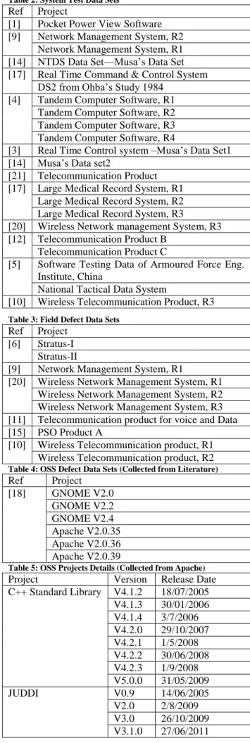
We have selected both system test and field defect data sets in order to evaluate the best fitting and best predictor SRGM for both system test and operation phase, because theTable 2: System Test Data Sets
Ref Project
[1] Pocket Power View Software [9] Network Management System, R2
Network Management System, R1 [14] NTDS Data Set—Musa’s Data Set [17] Real Time Command & Control System
DS2 from Ohba’s Study 1984 [4] Tandem Computer Software, R1
Tandem Computer Software, R2 Tandem Computer Software, R3 Tandem Computer Software, R4
[3] Real Time Control system –Musa’s Data Set1 [14] Musa’s Data set2
[21] Telecommunication Product [17] Large Medical Record System, R1
Large Medical Record System, R2 Large Medical Record System, R3
[20] Wireless Network management System, R3 [12] Telecommunication Product B
Telecommunication Product C
[5] Software Testing Data of Armoured Force Eng. Institute, China
National Tactical Data System
[10] Wireless Telecommunication Product, R3
Table 3: Field Defect Data Sets
Ref Project [6] Stratus-I
Stratus-II
[9] Network Management System, R1
[20] Wireless Network Management System, R1 Wireless Network Management System, R2 Wireless Network Management System, R3 [11] Telecommunication product for voice and Data [15] PSO Product A
[10] Wireless Telecommunication product, R1 Wireless Telecommunication product, R2
Table 4: OSS Defect Data Sets (Collected from Literature)
Ref Project [18] GNOME V2.0 GNOME V2.2 GNOME V2.4 Apache V2.0.35 Apache V2.0.36 Apache V2.0.39
Table 5: OSS Projects Details (Collected from Apache)
Project Version Release Date
C++ Standard Library V4.1.2 18/07/2005 V4.1.3 30/01/2006 V4.1.4 3/7/2006 V4.2.0 29/10/2007 V4.2.1 1/5/2008 V4.2.2 30/06/2008 V4.2.3 1/9/2008 V5.0.0 31/05/2009 JUDDI V0.9 14/06/2005 V2.0 2/8/2009 V3.0 26/10/2009 V3.1.0 27/06/2011
software reliability models are used for the prediction of failure in both phases and the phase may be a factor for model selection
.
Table 4 contains the list of OSS defect data sets. Six data sets contain defect data of two OSS Projects, Apache and GNOME. Three data sets have been collected from different versions of each of the two OSS projects.Apart from this we identified two notable and active open source projects from apache.org (https://issues.apache.org/). These projects are C++ Standard Library and JUDDI. The Apache C++ Standard Library provides a free implementation of the ISO/IEC 14882 international standard for C++ that enables source code portability and consistent behaviour of programs across all major hardware implementations, operating systems, and compilers, open source and commercial alike. JUDDI is an open source Java implementation of the Universal Description, Discovery, and Integration (UDDI v3) specification for (Web) Services. Both of these projects are considered stable in production. The 66% of the reported issues in first project have been fixed while in the second project 95% of the reported issues have fixed and closed. We collected defect data of the selected projects from apache.org using JIRA. JIRA is a commercial issue tracker. Issues can be bugs, feature requests, improvements, or tasks. JIRA track bugs and tasks, link issues to related source code, plan agile development, monitor activity, report on project status.
For each version found in the issue tracking system we have collected all the issues reported at our date of observation together with the date at which they were reported (date of opening). For each open source project, we have considered all the major versions until April 2012. For C++ Standard Library we were able to get eight (8) versions. Unfortunately, JUDDI had not so many reports and versions as compared to C++ Standard Library and we had to limit the versions to four (4) for JUDDI until October 2011. Table 5 lists the information of the projects.
After a deep inspection of the repositories and of their documentation, we have decided to focus on those issues that were declared “bug” or “defect” excluding “enhancement,” “feature-request,” “task” or “patch”. For the same reason, we have considered only those issues that were reported as closed or resolved (according to the terminology of the single repository) after the release date of each version. Further, we excluded issues closed before the release date. These issues are typically found in the candidate (or testing) releases of projects. The complete datasets are available online2.
V. RESULTS
RQ1: Which SRGM models fit best?
First we consider the basic capability of a model to fit the dataset (fits or not), irrespective of the goodness of fit (R2). Figure 1 reports for each model on the X axis the percentage of datasets fitted (axis Y) in each data group (colour bars). Musa Okumoto fitted to all data sets in each group, most models also fit, except Yamada exponential, Gompertz, Generalized Goel that fit poorly, especially field test and system test datasets.
Now let’s analyse goodness of fit too. Figure 2 reports how many times a model is the one with best R2. For instance
Musa Okumoto has the best R2 on 60% of field defect datasets. Musa Okumoto is top performer on field defects data; Gompertz has very good results on OSS datasets directly followed by Inflection S-Shaped Model. But apart from that there is no clear best model.
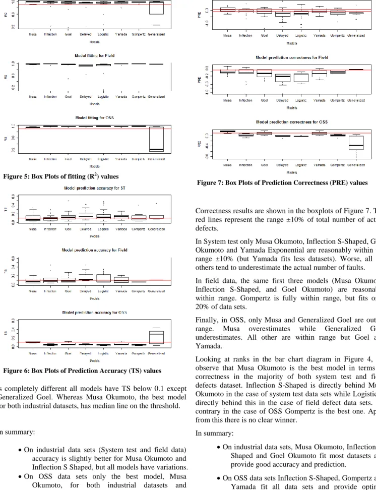
However, analysing the top performer only as in Figure 2 can be misleading, in case many models fit with a similar R2 the same dataset. Therefore in boxplots of Figure 5 we report the boxplots of R2 per model and per dataset category. It should be reminded however that boxplots of Figure 5 excludes the models that did not fit at all the datasets (Figure 1) and is therefore meaningful for all models except Yamada exponential, Gompertz, and Generalized Goel. Musa Okumoto remains the best performer (no outliers and narrow boxplot on all categories of datasets). Next to it the other models have also narrow boxplot (always better than 0.9, the threshold depicted as a colour horizontal line) but some outliers. It should be noted that all models behave extremely well (R2 close to 1 and no outliers) on the OSS datasets except Generalized Goel.
In summary:
Considering plain fitting (Fig 1), Musa Okumoto fits all datasets, Yamada exponential, Gompertz, Generalized Goel fit more OSS datasets but behave poorly on the others, the others fit at least 80% of the data sets
Considering the R2 of models that fit the datasets (Figure 5), Musa Okumoto has always a very good fit (better than 0.9), the others, except Generalized Goel, also perform quite well but with outliers.
RQ2. Which SRGM models are good predictors?
For models that could fit the data set we used the first two-third data points of the data sets to train the model, and predicted the last third. We analyse their predicting capability in terms of accuracy and precision.
Accuracy
Figure 3 shows the number of times a model is the best predictor in terms of TS. It is clear that Musa Okumoto outperforms the others in both the industrial datasets. The Logistic Model is directly behind it. On the contrary in the case of OSS we got several ties (this explains why the sum of percentage might be greater than 100%), and the best model is Gompertz directly followed by Logistic.
Figure 6 reports the TS values for all datasets. The red line represents the 0.1 threshold, usually considered indicator of good accuracy. Figure 6 allows us to discuss good models, instead of best model as in Figure 3.
In System Test data, all models show variations, however Musa Okumoto and Inflection S-Shaped have a median below the 0.1 threshold. This happens also for Gompertz and the Generalized Goel models; however they do not fit in several cases (Figure 1).
In Field data sets all models except Delayed S-Shaped have a median below the threshold, but indeed show variation. Musa-Okumoto is the first in 60% of datasets. In OSS the situation
Figure 5: No of DS for each Best Fitted Model
Figure 2: No of DS for each best Predictor Model – Accuracy (TS value)
Figure 3: No of DS for each best Predictor Model – Correctness (PRE value)
Figure 1: No of DS fitted by each Model
Figure 2: Ranking on Best Fitting-R2
Figure 3: Ranking on best prediction: TS
is completely different all models have TS below 0.1 except Generalized Goel. Whereas Musa Okumoto, the best model for both industrial datasets, has median line on the threshold.
In summary:
On industrial data sets (System test and field data) accuracy is slightly better for Musa Okumoto and Inflection S Shaped, but all models have variations.
On OSS data sets only the best model, Musa Okumoto, for both industrial datasets and Generalized Goel have TS above 0.1.
Correctness
Correctness results are shown in the boxplots of Figure 7. The red lines represent the range ±10% of total number of actual defects.
In System test only Musa Okumoto, Inflection S-Shaped, Goel Okumoto and Yamada Exponential are reasonably within the range ±10% (but Yamada fits less datasets). Worse, all the others tend to underestimate the actual number of faults. In field data, the same first three models (Musa Okumoto, Inflection S-Shaped, and Goel Okumoto) are reasonably within range. Gompertz is fully within range, but fits only 20% of data sets.
Finally, in OSS, only Musa and Generalized Goel are out of range. Musa overestimates while Generalized Goel underestimates. All other are within range but Goel and Yamada.
Looking at ranks in the bar chart diagram in Figure 4, we observe that Musa Okumoto is the best model in terms of correctness in the majority of both system test and field defects dataset. Inflection S-Shaped is directly behind Musa Okumoto in the case of system test data sets while Logistic is directly behind this in the case of field defect data sets. On contrary in the case of OSS Gompertz is the best one. Apart from this there is no clear winner.
In summary:
On industrial data sets, Musa Okumoto, Inflection S-Shaped and Goel Okumoto fit most datasets and provide good accuracy and prediction.
On OSS data sets Inflection S-Shaped, Gompertz and Yamada fit all data sets and provide optimal accuracy and prediction.
Figure 5: Box Plots of fitting (R2) values
Figure 6: Box Plots of Prediction Accuracy (TS) values
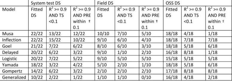
Table 2: Fitting and prediction capability of models
System test DS
Field DS
OSS DS
Model
Fitted
DS
R
2>= 0.9
AND TS
<0.1
R
2>= 0.9
AND PRE
within
0.1
Fitted
DS
R
2>= 0.9
AND TS
<0.1
R
2>= 0.9
AND PRE
within
0.1
Fitted
DS
R
2>= 0.9
AND TS
<0.1
R
2>= 0.9
AND PRE
within
0.1
Musa
22/22
13/22
12/22
10/10
7/10
5/10
18/18
4/18
1/18
Inflection
22/22
15/22
10/22
9/10
6/10
4/10
18/18
7/18
7/18
Goel
21/22
7/22
6/22
8/10
6/10
3/10
18/18
5/18
6/18
Delayed
20/22
6/22
3/22
9/10
1/10
2/10
16/18
8/18
1/18
Logistic
20/22
7/22
5/22
9/10
5/10
5/10
15/18
5/18
5/18
Yamada
18/22
3/22
4/22
5/10
2/10
1/10
18/18
5/18
6/18
Gompertz
14/22
6/22
3/22
2/10
2/10
2/10
17/18
8/18
8/18
Generalized 10/22
2/22
1/22
1/10
1/10
0/10
16/18
4/18
2/18
RQ3. A model with good fit is also a good
predictor?
Here we fit models on two thirds of the data sets and we analyse if the ones with good R2 are also good predictors. Table 5 reports models and data sets. A model is described by three cells per category of dataset. The first contains the number of times a model fits the dataset, with any R2 (information is also in Figure 1), the second shows how many times the model fits a data set with R2 better than 0.9 and predicts with TS < 0.1, the third shows how many times the model fits a data set with R2 better than 0.9 and predicts with PRE within 10%. . We observe from Table 5 that:
On industrial datasets, Musa and Inflection are the ones with better prediction capability – however this happens only in a bit more than half the datasets
On OSS datasets Gompertz and Inflection have good prediction capability for all datasets, followed by Logistic and Goel Okumoto.
VI.DISCUSSION
We have attempted to derive general conclusion about best fitter and best predicting SRGM model applying eight different models to a wide range of datasets on failures. Considering the three RQs the origin of datasets appears to be a factor. The performance of models differs slightly between System test and Field test datasets. Results show that models that have good performances in fitting and predicting in system tests are still good in fitting and predicting field defects. We think this is a very practical and important finding because quality and maintenance managers might choose only one model regardless of the phase of the software lifecycle data come from.
Yet another interesting fact from the analysis is that there is a clear difference between OSS and industrial data sets. The best performer models are Musa Okumoto and Inflection for industrial datasets, while Gompertz is the best for OSS datasets followed by Inflection S-Shaped Model. This is due to the fact that these models are S-shaped and apply better to the fitted data. It might indicate an initial learning phase in which the community of end-users and reviewers of the open source project does not react promptly to the new release. Yet
another explanation could be that OSS datasets are significantly different from industrial datasets (there is no distinction between System Test failures and Field defects), so we cannot really derive any meaningful consequence.
We finalize this discussion with a message to the maintenance and quality manager that might read this analysis. We provided ranks and boxplots to show to the readers that certain models got good fitting\prediction performances in several datasets. Although the high number of datasets used (50) might make our findings generalizable, we strongly suggest the reader to define her own thresholds for fitting, accuracy and correctness of predictions and re elaborate the results according to those thresholds, using the boxplot provided. In fact we are convinced that each context has unique combination of characteristics that make some thresholds more appropriate than others, thus the choice of the SRGM should be based on characteristics of the context and the data it is going to be applied.
VII. THREATS TO VALIDITY
We recognize a first conclusion threat in the methodology we used to answer research questions, because we did not apply hypothesis testing due to the low cardinality of some datasets. Moreover the choice of threshold is also not grounded in the literature.
This approach was conscious and deliberate though. We preferred to choose indicative thresholds and show all boxplots to not bias the reader: we strongly believe that classifying a model as good or bad is a task that strictly depends on the level of performances that the manager wants to achieve. Each reader might decide by herself whether the threshold we used is appropriate for her context or not, and classify differently the models by looking at the boxplots. However, we did not leave this threat uncontrolled and we provided the reader with ranks to identify the best model for each type of datasets and metric.
We observe a construct threat in the impossibility to adequately compare industrial datasets with OSS datasets due to the lack of information on the defect detection phase (system test, operation) in latter one: we could not build a proper control strategy except avoiding a structured comparison between industrial and OSS results.
We notice a conclusion threat in the choice of not performing cross validation in prediction. However we grounded our choice in the literature.
Finally, an external threat is the low number of datasets in for field defects. However Apache and GNOME projects both have large and well organized communities, where a great number of developers contribute to the projects. The large sizes of these two projects make them the state-of-the-art in terms of management of OSS projects.
VIII. CONCLUSIONS
We have studied selected SRGM in generalized way for the purpose to derive general conclusion. In the literature nobody has validated the SRM in such generalized way: at maximum four/five models are validated on two/three datasets [42, 4, 17]. We found that the Musa-Okumoto model is the best one in fitting and predictions in industrial datasets. Although also Inflection S-Shaped achieved very good results with respect to the metrics thresholds we adopted. The Musa-Okumoto model did not hold the same performances in OSS data, in which the Gompertz model applied better, followed by Inflection S-Shaped.
We also observed two other interesting facts: 1) models which have good performances with system test data sets also good performances with field defect data, and 2) models that fit very well system test data not always predict with same
performances. The practical consequences and
recommendations to quality and maintenance managers are: 1) choose only one model regardless of the phase of the software lifecycle, 2) identify and choose a model that is flexible enough in case the quality process is under definition or in generable susceptible of important changes.
Our future work will be devoted to the extension of the datasets used to increase the generalizability of these findings, especially in OSS projects where results and structure of datasets were very different from industrial ones.
REFERENCES:
[1] Arora, S. et al, “Software Reliability Improvement through Operational Profile Driven Testing”, Proceedings Reliability and Maintainability Symposium, 2005.
[2] Goel, A. L., and Okumoto, K. 1979. “A time dependent error detection model for software reliability and other performance measures”, IEEE Transactions on Reliability 28(3): 206–211.
[3] Xuemei Zhang, et al, “Considering Fault Removal Efficiency in Software Reliability Assessment”, IEEE Transactions on Systems, Man, and Cybernetics—PART A: System and Human, Vol. 33, No. 1, January 2003 [4]Wood, Alan, “Software-reliability growth model: primary-failures generate secondary-faults under imperfect debugging and. IEEE Transactions on Reliability, 43, 3, 408 (September 1994).”
[5] Yongqiang Zhang, et al, “Improved Genetic Programming Algorithm Applied to Symbolic Regression and Software Reliability Modeling”, Journal of Software Engineering and Applications, pages 354-360, 2009
[6] Mullen, Robert E, “The Lognormal Distribution of Software Failure Rates: Application to Software Reliability Growth Modeling Cisco Systems 250 Apollo Road”.
[7] Kececioglu, D. 1991. Reliability Engineering Handbook, Vol. 2, Englewood Cliffs, NJ: Prentice-Hall.
[8] Lyu, M. (ed.): 1996, Handbook of Software Reliability Engineering. New York: McGraw-Hill.
[9] Jeske, Daniel R., et al, “Adjusting Software Failure Rates That Are Estimated from Test Data”, IEEE Transaction on Reliability, Vol. 54, No. 1, March 2005.
[10] Jeske, D.R., et al, “Accounting for Realities When Estimating the Field Failure Rate of Software”, Proceedings of 12th International Symposium on
Software Reliability Engineering, 2001.
[11] Jeske, D.R., et al, “Estimating the failure rate of evolving software systems”, Proceedings 11th International Symposium on Software Reliability Engineering, 2000.
[12] Derriennic, H., Le Gall, G., “Use of failure-intensity models in Software-validation Phase for Telecommunications”, IEEE Transaction on Reliability, Vol. 44, No. 4, 1995 December.
[13] Musa, J., Iannino, A., and Okumoto, K. 1987. Software Reliability: Measurement, Prediction, Application. New York: McGraw-Hill.
[14] Cao, Yong. , Zhu, Qingxin, “The Software Failure Prediction Based on Fractal”, Journal Advanced Software Engineering and Its Applications, Pages 85-90, 2008.
[15] Jalote, Pankaj, et al, “Post-release reliability growth in software products”, ACM Transactions on Software Engineering and Methodology, Vol. 17, Pages 1-20, 2008.
[16] Trachtenberg, M. 1990, “A general theory of software-reliability modeling”, IEEE Transactions on Reliability 39(1): 92–96.
[17] Lo, J., Huang, C., “An integration of fault detection and correction processes in software reliability analysis”, Journal of Systems and Software, Vol.79, Pages 1312-1323, 2006.
[18] Li, Xiang, et al, “Reliability analysis and optimal version-updating for open source software”, Journal of Information and Software Technology, Vol. 53, Pages 929-936, 2011.
[19] Yamada, S., Ohba, M., and Osaki, S. 1983. “S-shaped reliability growth modeling for software error detection”, IEEE Transactions on Reliability 32(5): 475–478.
[20] Jeske, D, “Some successful approaches to software reliability modeling in industry”, Journal of Systems and Software, Vol. 74, Pages 85-99, 2005. [21] Kelani Bandara, K.B.P.L.M. et al, “Optimal selection of failure data for reliability estimation based on a standard deviation method”, Proceedings of International Conference on Industrial and Information Systems, 2007. [22] Yamada, S., Ohtera, H., and Narihisa, H. 1986. Software reliability growth models with testing effort. IEEE Transactions on Reliability 35(1): 19–23.
[23] Stringfellow, C, et al, “An Empirical Method for Selecting Software Reliability Growth Models”, pages 1-21.
[24] Musa, J., and Ackerman, A. 1989, Quantifying software validation: When to stop testing. IEEE Software. 19–27
[25] Wood, A. 1996, Predicting software reliability. IEEE Computer 29(11): 69–78.
[26] Wood, A. 1997. Software reliability growth models: Assumptions vs. reality. Proceedings of the International Symposium on Software Reliability Engineering 23(11): 136–141.
[27] J. D. Musa and K. Okumoto, “A logarithmic Poisson execution time model for software reliability measurement,” in Conf. Proc. 7th International Conf. on Softw. Engineering, 1983, pp. 230–237.
[28] C. Y. Huang, M. R. Lyu, and S. Y. Kuo, “A unified scheme of some non-homogenous Poisson process models for software reliability estimation,”
IEEE Trans. Softw. Engineering, vol. 29, no. 3, pp. 261–269, March 2003. [29] Kapil Sharma, et al, “Selection of Optimal Software Reliability Growth Models Using a Distance Based Approach”, IEEE TRANSACTIONS ON RELIABILITY, VOL. 59, NO. 2, JUNE 2010
[30] J. D. Musa, A. Iannino, and K. Okumoto, Software Reliability Measurement, Prediction, Application. : McGraw Hill, 1987
[31] G. H. Schick and R. W. Wolverton, “An analysis of competing software reliability models,” IEEE Trans. Software Engineering, pp. 104–120, March 1978.
[32] A. N. Sukert, “Empirical validation of three software errors predictions models,” IEEE Transaction on Reliability, pp. 199–205, August 1979. [33] S. Brocklehurst, P. Y. Chan, B. Littlewood, and J. Snell, “Recalibrating software reliability models,” IEEE Trans. Softw. Engineering, vol. SE-16, no. 4, pp. 458–470, April 1990.
[34] A. L Goel, “Software reliability models: assumption, limitations, and applicability,” IEEE Transaction on Software Engineering, pp. 1411–1423, December 1985.
[35] Abdel-Ghaly, P.Y. Chan, and B. Littlewood, “Evaluation of competing software reliability predictions,” IEEE Trans. Softw. Engineering, vol. SE-12, no. 12, pp. 950–967, September 1986.
[36] T. M. Khoshgoftaar, “On model selection in software reliability,” in 8th Symposium in Computational Statistics, August 1988, pp. 13–14, (Compstat ’88).
[37] T. M. Khoshgoftaar and T. G. Woodcock, “A simulation study of the performance of the Akaike information criterion for the selection of software reliability growth models,” in Proc. of the 27th Annual South East Region ACM Conf., April 1989, pp. 419–423.
[38] T. M. Khoshgoftaar and T. Woodcock, “Software reliability model selection: A case study,” in Proc. of the 2nd International Symposium on Software Reliability Engineering. Austin, TX: IEEE Computer Society Press, 1991, pp. 183–191.
[40] K. Pillai and V. S. S. Nair, “A model for software development effort and cost estimation,” IEEE Transaction on Software Engineering, vol. 23, no. 8, pp. 485–497, 1997.
[41] K. C. Chiu, Y. S. Huang, and T. Z. Lee, “A study of software reliability growth from the perspective of learning effects,” Reliability Engineering and System Safety, pp. 1410–1421, 2008.
[42] Carina Andersson , “A replicated empirical study of a selection method for software reliability growth models”, journal of Empirical Software Engineering, pages 161-182, year 2006
[43] Syed-Mohamad et al, “Reliability Growth of Open Source Software Using Defect Analysis”, International Conference on Computer Science and Software Engineering, 2008.
[44] Ying Zhou et al, “Open source software reliability model: an empirical approach”, ACM SIGSOFT Software Engineering Notes, 2005
[45] Bruno Rossi et al, “Modelling Failures Occurrences of Open Source Software with Reliability Growth”, journal of Open Source Software: New Horizons, page 268-280, 2010.
[46] Cobra Rahmani et al, “A Comparative Analysis of Open Source Software Reliability”, Journal of Software, page 1384-1394, 2010.
[47] IEEE Std 1633-2008 IEEE Recommended Practice in Software Reliability
[48] Basili, et al, "The Goal Question Metric Approach", in Encyclopedia of Software Engineering, Wiley, 1994.
[49] http://www.cse.cuhk.edu.hk/~lyu/book/reliability/
[50] O. Gaudoin et al, “A simple goodness of fit test for the power law process based on the Duane plot”,IEEE Transactions on Reliability