Effect of the Spin Orbit Interaction (Heisenberg XYZ Model) on Partial Entangled Quantum Network

http://dx.doi.org/10.4236/jqis.2014.41001

Effect of the Spin-Orbit Interaction

(Heisenberg XYZ Model) on Partial

Entangled Quantum Network

Abdel-Haleem Abdel-Aty1, Nordin Zakaria1, Lee Yen Cheong2, Nasser Metwally3 1_{Computer and Information Science Department, Universiti Teknologi Petronas, Tronoh, Malaysia} 2_{Fundamentals and Applied Science Department, Universiti Teknologi Petronas, Tronoh, Malaysia} 3_{Mathematics Department, College of Science, University of Bahrain, Sakhir, Kingdom of Bahrain} Email: [email protected], [email protected]

Received 16 November 2013; revised 6 January 2014; accepted 28 January 2014

Copyright © 2014 by authors and Scientific Research Publishing Inc.

This work is licensed under the Creative Commons Attribution International License (CC BY).

http://creativecommons.org/licenses/by/4.0/

Abstract

Dzyaloshiniskii-Moriya (DM) interaction in three directions (Dx, Dyand Dz) is used to generate en-

tangled network from partially entangled states in the presence of the spin-orbit coupling. The ef- fect of the spin coupling on the entanglement between any two nodes of the network is investi- gated. The entanglement is quantified using Woottores concurrence method. It is shown that the entanglement decays as the coupling increases. For larger values of the spin coupling, the entan- glement oscillates within finite bounds. For the initially entangled channels, the upper bound does not exceed its initial value, whereas the entanglement reaches its maximum value for the channels generated via indirect interaction.

Keywords

Quantum Network; Entanglement; Spin-Orbit Interaction

1. Introduction

quantum networks increased in the past few years in regards to the problems in the classical networks like the security of the information, privacy and the speed of the transmission of information. Quantum networks have been implemented experimentally [11]-[14] and theoretically [15]-[19].

The Dzyaloshiniskii-Moriya (DM) interaction is a natural phenomena discovered in 1960 by Moriya Dzya- loshinskii-Moriya (DM) as an antisymmetric and anisotropic exchange coupling between two spins) [20] [21]. It is found that the DM interaction strengthen the entanglement among particles implies that the DM interaction plays an important role in the generation of the quantum entanglement in the field of quantum networks [22]. The quantum correlation as a result of the DM interaction between two particles is investigated by many authors (see for examples [23]-[25]). The thermal entanglement between two qubits in the Heisenberg XYZ model and the effect of the DM interaction and its strength are discussed by Da Chuang and Z. Liang Cao [26]. The effect of the intrinsic decoherence in the teleportation of two qubits XYZ model is studied in the presence of DM inte- raction [27]. Entanglement sudden death and birth of the qubit-qutrit pair under DM interaction [28] and the ef- fect of the spin-orbit interaction in the dynamics of the entanglement in the presence of DM interaction [29]-[31]

are investigated recently.

Metwally [15] introduced a theoretical protocol to generate multi-nodes quantum network by using maximum entangled states, where the terminals of each disconnected node are connected via DM interaction. Theoretical quantum network model with “d” level system is constructed and gives important results in many useful appli- cations in quantum network environment [32]. The possibility of generating entangled network by using a class of partially entangled network is discussed by Abdel-Aty et al.[16]. Also, as a development of our last quantum network we studied the possibility of the generation of quantum network with the DM interaction is switched to more than one direction. The quantum teleportation is investigated over this quantum network as well [17]. Therefore, we are motivated to investigate the effect of the spin-orbit and the efficiency of the generated entan- gled network in the presence of DM interaction.

In this paper, we introduce the model and its evolution in Section 2. The entanglement between different nodes is quantified for different values of the spin-orbits coupling and the DM’s strength is discussed in Section 3. We then summarize our results and discussion in Section 4.

2. The Model

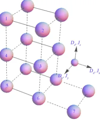
It is assumed that entangled network consists of four nodes is generated by using partial entangled states of Werner type [16] [33]. In the suggested quantum network the node “1” and node “2” is initially connected as well as node “3” and “4” (solid line). The dash line between the node “2” and node “3” represents the connec- tions which generated by the DM (x, y and z) interaction with the effect of the spin orbit coupling Jx, Jy and Jz

as seen in Figure 1.

Consider a partial entangled state generated by a source of the form 4 1 1 3 3 w w ij F F I

ρ ₌ − ₊ − ψ− ψ−

(1)

where 1

(

)

2

ψ− _{= −}

is the singlet Bell state and Fw is the maximum fraction corresponding to the

Werner-state.

The initial state of the total system is given by

( )

1234 0 12 34

ρ =ρ ⊗ρ (2)

The evolution of the initial state (2) is given by,

( )

( )

( )

( )

1234 t DM t 1234 0 DM t

ρ = ρ  (3)

where D_M

( )

( )

M

i t D t

−

= 

 (4)

where M D

 is the Hamiltonian of the DM (x, y and z) interaction which rules the interactions as you will see in Sections (2.1, 2.2 and 2.3).

2.1. Heisenberg XYZ Model with Dx

The Hamiltonian describing the evolution of the system for a two-qubit spin-orbit chain with the DM interaction is switched on the x-axis can be written as

( ) ( ) ( ) ( ) ( ) ( )

( ) ( ) ( )

(

)

x

k l k l k l

D x x x y y y z z z

k l k l

x y z z y

J J J

D

σ σ σ σ σ σ

σ σ σ σ

= + +

+ −



(5)

where k, l represent the nodes which are connected together via DM interaction with x-component of strength Dx; Jx, Jy and Jz are the x, y and z-component of the real coupling coefficients, respectively, and the σ σ( ) ( )_xk _xl is the

Pauli matrices σx = 1 0 + 0 1 , σy =i

(

)

The final density operator of the network is given by

( )

( )

( )

( )

1234 t Dx t 1234 0 Dx t

ρ = ρ  (6)

where

( )

x

i t D t

−

= 

 (7)

is the unitary operator which can be written explicitly in the basis 00, 01,10,11 as

( )

ee ee ee eg ee ge ee gg

eg ee eg eg eg ge eg gg D

ge ee ge eg ge ge ge gg

gg ee gg eg gg ge gg gg

u u u u

u u u u

t

u u u u

u u u u

      =        

 (8)

where

( )

( )

(

)

( )

(

( )

( )

( )

( )

)

( )

(

)

, sin cos sin sin sin cos cos cos sin ( ) ,

ge eg z z x x y x y x x y

u = i J t + J t _ D t − J t J t + J t J t − D t J +J t _

( )

( )

(

)

( )

(

( )

( )

( )

( )

)

( )

(

(

)

)

, sin cos cos sin sin cos cos sin sin ,

ge ge z z x x y x y x x y

u = i J t + J t _ D t − J t J t + J t J t − D t J +J t _

( )

(

( )

( )

)

(

( )

( )

)

(

( )

( )

)

,

1

sin sin cos sin cos sin cos ,

2

ge gg x x x y y z z

( )

(

( )

( )

)

(

( )

( )

)

(

( )

( )

)

,

1

sin sin cos sin cos sin cos ,

2

gg ge x x x y y z z

u =− D t i J t + J t i J t − J t i J t − J t

( )

( )

(

)

( )

(

( )

( )

( )

( )

)

( )

(

(

)

)

, sin cos sin sin sin cos cos cos sin ,

gg ee z z x x y x y x x y

u = −i J t + J t _ D t J t J t + J t J t − D t J −J t _

( )

( )

(

)

( )

(

( )

( )

( )

( )

)

( )

(

(

)

)

sin cos cos sin sin cos cos

sin sin ,

gg gg z z x x y x y

x x y

u i J t J t D t J t J t J t J t

i D t J J t



= − + _ +



− − _

And the rest of the components uge ee, = −uge gg, , ugg eg, = −ugg ge, =uee eg, = −uee ge, , uge ge, =ueg eg, , uge eg, =ueg ge, , , ,

gg ee ee gg

u =u and uee ee, =ugg gg, . Using Equations (6) and (8), one obtains the final entangled network between

four nodes. Since that we are interested to quantify the degree of entanglement between different nodes, one can obtain the required density operator between each pair of nodes by tracing out the other two. For example, the density operator between the first and the second node is given by ρ12

( )

{

( )

}

2.2. Heisenberg XYZ Model with Dy

Similarly, the Hamiltonian describing the evolution of the system when the interaction is switched to the

y-direction can be written as.

( ) ( ) ( ) ( ) ( ) ( )

(

)

y

k l k l k l k l k l

D =Jxσ σx x +Jyσ σy y +Jzσ σz z +Dy σ σz x −σ σx z

 (9)

In this case, the unitary operator is given by

( )

i t D t

−

= 

 (10)

In matrix form, the unitary operator Equation (10) can be written as a matrix Equation (8) and the elements of the matrix are:

( )

( )

(

)

( )

(

( )

( )

( )

( )

)

( ) (

(

)

)

sin cos sin sin sin cos cos

cos sin ,

ge eg z z y x y x y

y x y

u i J t J t D t J t J t J t J t

i D t J J t

 = + _ − +  − + _

( )

( )

(

)

( )

(

( )

( )

( )

( )

)

( ) (

(

)

)

sin cos cos sin sin cos cos

sin sin ,

ge ge z z y x y x y

y x y

u i J t J t D t J t J t J t J t

i D t J J t



= + _ − +



− + _

(

)

(

( )

( )

)

(

( )

( )

)

(

( )

( )

)

, sin 2 sin cos sin cos sin cos ,

2

ge gg y x x y y z z

i

u =− D t i J t + J t i J t + J t i J t + J t

(

)

(

( )

( )

)

(

( )

( )

)

(

( )

( )

)

, sin 2 sin cos sin cos sin cos ,

2

gg ge y x x y y z z

i

u =− D t i J t − J t i J t + J t i J t − J t

( )

( )

(

)

( )

(

( )

( )

( )

( )

)

( )

(

(

)

)

sin cos sin sin sin cos cos

cos sin ,

gg ee z z y x y x y

x x y

u i J t J t D t J t J t J t J t

i D t J J t

 = − + _− +  − − _

( )

( )

(

)

( )

(

( )

( )

( )

( )

)

( ) (

(

)

)

sin cos cos sin sin cos cos

sin sin ,

gg gg z z y x y x y

y x y

u i J t J t D t J t J t J t J t

i D t J J t



= − + _ +



+ − _

And the rest of the components u_{ge ee,} =u_{ge gg,} =u_{eg gg,} =u_eg,ee , u_{gg ge,} = −u_{gg eg,} =u_{ee eg,} = −u_{ee ge,} ,

, ,

ge ge eg eg

u =u , u_{ge eg,} =u_{eg ge,} , u_{gg ee,} =u_{ee gg,} and u_{ee ee,} =u_{gg gg,} .

2.3. Heisenberg XYZ Model with Dz

z-direction can be written as.

( ) ( ) ( ) ( ) ( ) ( )

(

)

z

k l k l k l k l k l

D =Jxσ σx x +Jyσ σy y +Jzσ σz z +Dz σ σx y −σ σy x

 (11)

In this case, the unitary operator is given by

( )

z

i t D t

−

= 

 (12)

Is the unitary operator which used to connect between particle “2” and “3” when the interaction is switched on y-axis and defined by

( )

( )

_{( )}

( )

( )

_{( )}

_{( )}

( )

( )

_{( )}

(

)

₍

₎

2 3 2 3 2 3

23

2 3 2 3 2 3

2 2 2

cos sin cos sin cos sin

cos cos sin sin 2

2 z

D x x x x y y y y z z z z

z z z z z x y y x z

t J t i J t J t i J t J t i J t

i

D t D t i D t D t

σ σ σ σ σ σ

σ σ σ σ σ σ

      =_ − _{ }× − _{ }× − _   ×_ + − − _    (13)

In matrix form, the unitary operator Equation (13) can be written as in Figure 8. Where the elements of the matrix are:

( )

( )

(

)

(

)

(

( )

( )

( )

( )

)

(

)

(

(

)

)

, sin cos cos 2 sin sin cos cos

sin 2 sin ,

eg eg z z z x y x y

z x y

u i J t J t D t J t J t J t J t

i D t J J t

 = + _ − +  − + _

( )

( )

(

)

(

)

(

( )

( )

( )

( )

)

(

)

(

(

)

)

, sin cos sin 2 sin sin cos cos

cos 2 sin ,

eg ge z z z x y x y

z x y

u i J t J t D t J t J t J t J t

i D t J J t

 = + _− − +  − + _

( )

( )

(

)

(

)

(

( )

( )

( )

( )

)

(

)

(

(

)

)

, sin cos sin 2 sin sin cos cos

cos 2 sin ,

ge eg z z z x y x y

z x y

u i J t J t D t J t J t J t J t

i D t J J t

 = + _− +  − + _

( )

( )

(

)

(

)

(

( )

( )

( )

( )

)

(

)

(

(

)

)

, sin cos cos 2 sin sin cos cos

sin 2 sin

ge ge z z z x y x y

z x y

u i J t J t D t J t J t J t J t

i D t J J t

 = + _ − +  + + _

(

)

(

)

(

( )

( )

)

, sin sin cos ,

gg ee x y z z

u =i J −J t i J t − J t

( )

( )

(

)

(

( )

( )

( )

( )

)

, sin cos sin sin cos cos ,

gg gg z z x y x y

u = −i J t + J t _ J t J t + J t J t _

And the rest of the components u_{gg gg,} =u_{ee ee,} , u_{gg ee,} =u_{ee gg,} and

, , , , , , , , 0

gg ge gg eg ge gg eg gg ge ee eg ee ee ge ee eg

u =u =u =u =u =u =u =u =

3. Results and Discussion

In this section, we quantify the entanglement between each pair of nodes. Practically, we consider the channels

( )

ij t

ρ , where ij = 12,13 and 14. For this purpose, we use Wootters’s concurrence as a measure for the entan- glement [34] which is defined by

{

}

max λ λ λ λ , 0

= − − −

 (14)

where λk (k = 1, 2, 3, 4) is the eigen values of the matrix

( ) ( )

(

)

(

)

.

i l i j

ij y y ij y y

ρ σ ⊗σ ρ σ ⊗σ

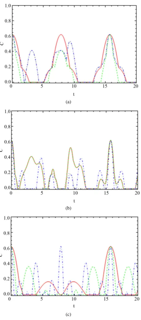
The entanglement behavior (concurrence) of the entangled state between nodes “1” and “2”, ρ12, is de-

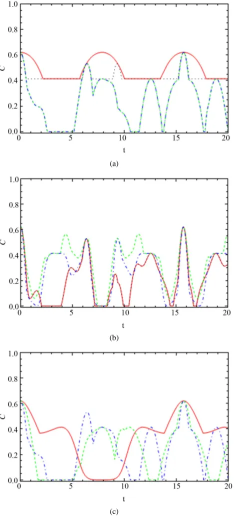
scribed in Figure 2 for different coupling values Ji (i= x, y, z), and the strength of DM is assumed to be fixed, Dx = 0.2. Figure 2(a) depicted the evolution of the concurrence C in the presence of zero coupling or one and only one non-zero coupling. In this case, the hamiltonian will be convert to

(

)

x

k l k l

D =Dx σ σy z −σ σz y

 . It is clear

(a)

(b)

(c)

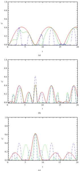
Figure 2. The entanglement, C12, between node “1” and node

“2” (a) the solid red line for Jx = Jy =Jz= 0 without the effect of

spin), the black dotted line for (Jx = 0.5 and Jy = Jz = 0,) green

line for (Jy = 0.5 and Jx = Jz = 0), blue dashed line for ( Jx = Jy

=0 and Jz = 0.5) and Dx = 0.2. (b) Similar to (a) but the solid red

line for (Jx = Jy= 0.5 and Jz = 0), black dotted for (Jx = Jy = 0.5

and Jz= 0), green line for (Jx= 0 and Jy = Jz = 0.5), blue dashed

for (Jx = Jy = Jz= 0.5) and Dx = 0.2. (c) The red line represents

the entanglement for (Jx = Jy = Jz = 0.1), green dashed for (Jx =

Jy = Jz = 0.3) and the blue dashed line for (Jx = Jy = Jz = 0.5) and

tween the second and third node, and consequently some correlations are lost. However, the upper and lower bounds will depend on the non-zero coupling when it is switched on. This behavior shows that the minimum bound of C for Jx ≠ 0 is always larger than that depicted for Jy ≠ 0 or Jz ≠ 0. On the other hand, the concurrence

vanishes completely for Jy ≠ 0 or Jz≠ 0, i.e., C = 0 as the scaled time increased without exceeding the initial up- per limit [13] [14]. In Figure 2(c), we investigate the behavior of the concurrence for Jx= Jy= Jz≠ 0. It can be seen that when the coupling parameters are small, Jx= Jy= Jz= 0.1, the concurrence C decays gradually and va- nishes when t∈

{ }

Figure 2(b) describes the behavior of the concurrence for the entangled state ρ12, where two non-zero

couplings are considered. The general behavior is similar to the one that is depicted in Figure 2(a), but the number of oscillation increased within the bounds. If we compare the solid curves in the Figures 2(a) and (b), we see that the presence of the coupling causes the concurrence to decay quicker.

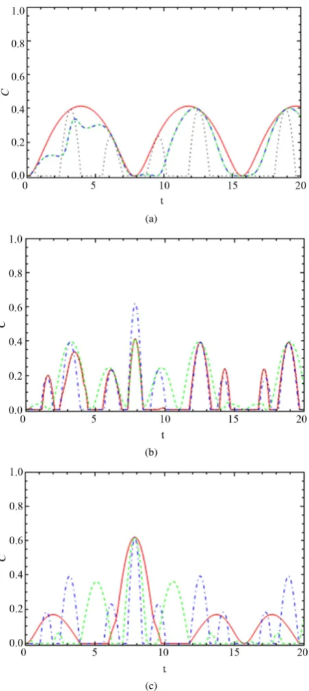
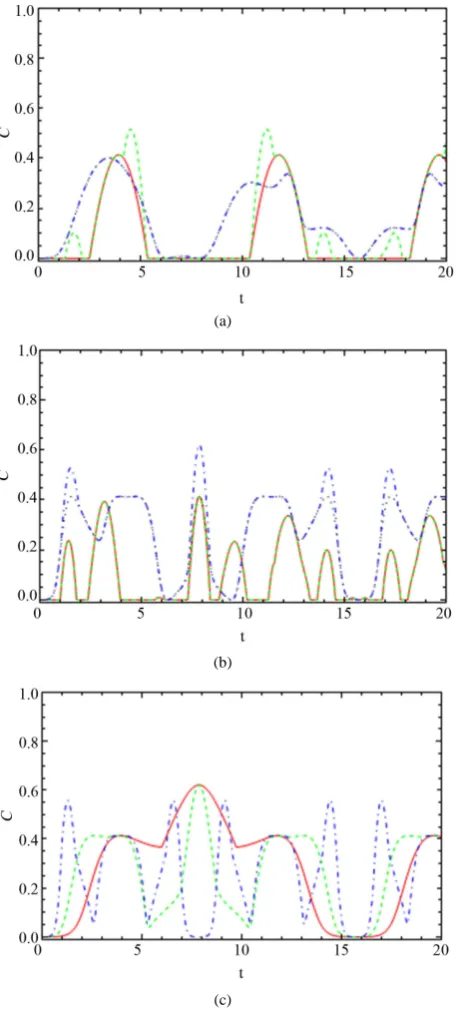
Figure 3 describes the behavior of the concurrence for the entangled state which is generated between nodes “1” and “3” via indirect interaction. Figure 3(a) describes the behavior of C for non-zero coupling where the same values of the coupling and DM’s strength as considered in Figure 2 are being used. Since the two nodes are initially disentangled, the concurrence C = 0 at t = 0. As soon as the interaction is switched on and the en- tangled state is generated between the first and the third node, the concurrence increased towards the upper bound (C = 0.4). As t continues to elapse, the concurrence decays and vanishes completely. This behavior is re- peated periodically.

The dynamics of concurrence, C, for the channel ρ13, when two non-zero couplings are considered is de-

picted in Figure 3(b). The values of Ji, where i = x, y, z are the same as in Figure 2(b). This figure shows that the concurrence oscillates between bounded limits. The phenomena of the sudden-death and sudden-birth ap- peared in the entanglement are shown clearly.

Figure 3(c) describes the behavior of C for the state ρ13 when Jx = Jy = Jz≠0have the same values as in Figure 2(c). It is clear that the general behavior is similar to that as depicted inFigure 3(b), but the number of oscillation increased as the value of the coupling increased. We note that the upper bound is slightly larger when

Jiis large.

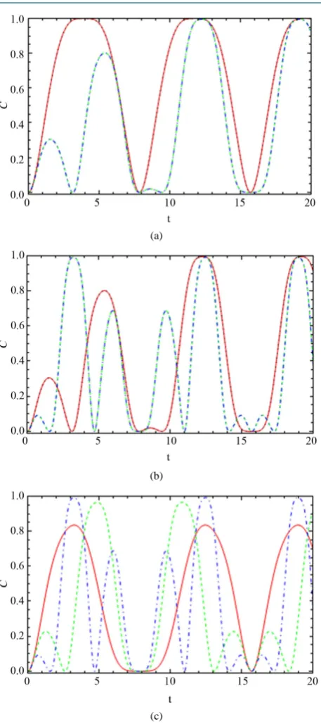
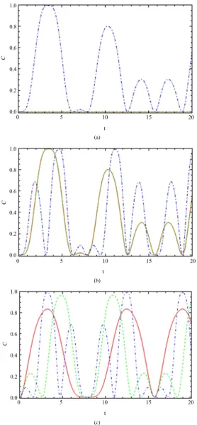
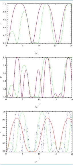
We investigate the behavior of the entanglement for state ρ14 generated via indirect interaction, is shown in

Figures 4(a)-(c). It is clear that the behavior of C is similar to that displayed for ρ13. However, the upper bound

for the state ρ14 is much larger and reaches maximum value at C = 1. The number of oscillation of the concur-

rence increased as the spin-orbit coupling increased.

On the other hand, the oscillation increased if all the couplings have non-zero values.

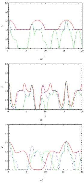
The dynamics of the entanglement in the quantum network when the interaction is switched on y-direction is shown in Figures 5-7. Figure 5 represents the entanglement over channel “12” with different values of the spin-orbit coupling. The parameters used in Figure 5(a) are identical to the one used in Figure 2(a) but the in- teraction is switched on y-axis with fixed Dy = 0.2. It is shown that when Jx = Jy = Jz = 0, the Hamiltonian represents the normal case without the effect of spin-orbit coupling has the form D_y =Dy

(

)

is represented by the solid red line [16]. The black dotted line illustrates the effect of the spin-orbit at Jx= 0.5 and Jy= Jz= 0. It is shown that the concurrence started from the maximum value at C = 0.62 and the entangle- ment decreased quickly as time goes on. The effect of spin-orbit Jz= 0.5 is shown by the dotted blue line which is similar to the black dotted line. The green dashed line represents the effect of Jy= 0.5 and Jx= Jz= 0. The en- tanglement shows similar behavior to the case when spin-orbit effect is ignored but a slight different to the am- plitude of the entanglement.

Figure 5(b) shows the effect of the spin-orbit interaction in two different directions. In this figure, the curves is initially started from its maximum and then the entanglement decreased to zero at t = 1. Then, the entangle- ment is increased again and reaches C = 0.4 at t = 2.5. One observes that the entanglement is influenced by the spin-orbit and the number of oscillations is increased.

The effect of Jx, Jyand Jzin the dynamics of the entanglement over channel “12” is depicted in Figure 5(c). This figure shows that the dynamics of the entanglement can be influenced by the values of the total spin-orbit interaction where the oscillation is increased by increasing the value of the spin-orbit. Here the solid red line represents the dynamics of the entanglement for Jx= Jy= Jz= 0.1, the dashed green line is produced by Jx= Jy=

Jz= 0.3 and the dotted blue line is produced by Jx = Jy = Jz = 0.5.

(a)

(b)

(c)

Figure 3.The dynamics of the entanglement, C13, between node “1” and node “3”. Figures (a), (b) and (c) have the same feature with Figure 2 but reside in channel “13”.

(a)

(b)

(c)

Figure 4. The dynamics of the entanglement, C14, between

node “1” and node “4”. Figures (a), (b) and (c) have the same feature with Figure 2but reside in channel “14”.

(a)

(b)

(c)

Figure 5. The dynamics of the entanglement, C12, between

node “1” and node “2”. (a), (b) and (c) are the same with Fig- ure 2 but the interaction switched on y-axis Dy = 0.2.

This figure shows the new feature is observed as the spin-orbit and the number of oscillations increased. Figures 7(a)-(c) show the entanglement dynamics between node “1” and node “4”. In Figure 7(a), we see that the spin-orbit interaction contributes to the x- and z-direction where the maximum value without the effect of the spin interaction is 4 × 1016 (solid red line), and with effect of the x- and z-spin-orbit the entanglement reaches a maximum of 1 at t = 3.

(a)

(b)

(c)

Figure 6. The dynamics of the entanglement, C13, between

node “1” and node “3”. (a), (b) and (c) are the same with Fig- ure 3but the interaction switched on y-axis Dy = 0.2.

can see in the red and dashed green lines for Jx= Jy= 0.5 and Jy = Jz= 0.5, respectively. The dotted black line and dotted blue line are the combination of the spin-orbit interaction in x- and z-direction which leads to the in- creasing in the entanglement oscillations. The effect of the spin-orbit affects the entanglement dynamics on channel “14” (see Figure 7(c)) where increasing the spin-orbit value leads to the number of oscillations in- creased.

(a)

(b)

(c)

Figure 7. The dynamics of the entanglement, C14, between node “1” and

(a)

(b)

(c)

Figure 8. The dynamics of the entanglement, C12, between node “1” and

(a)

(b)

(c)

Figure 9. The dynamics of the entanglement, C13, between node “1” and

(a)

(b)

(c)

Figure 10. The dynamics of the entanglement, C14, between node “1”

and node “4”. (a), (b) and (c) are the same feature with Figure 4 but the interaction switched on y-axis Dz= 0.2.

4. Conclusions

We discussed the effect of the spin-orbit (Heisenberg XYZ model) coupling to the entanglement between dif- ferent nodes in the quantum network. It is shown that the entanglement decays for nonzero coupling. The phe- nomena of the entanglement sudden-death and sudden-birth appeared for larger coupling values. It shows that the coupling constant of the entangled channel initially has no effect on the upper bound of the entanglement. However, the lower bound of the entanglement does not vanish for non-zero couplings. The number of oscilla- tions is increased as the coupling is increased. For entangled channels which are generated either via direct or indirect interactions, the concurrence and the number of oscillations are increased as the coupling is increased.

Finally, it is shown that the generated entangled channel between any two nodes via indirect interaction has a large degree of entanglement and the upper bound exceeds the initial entangled state. Therefore, one may gene- rate maximum entangled state from the less entangled state by controlling the spin-orbit coupling. This means that terminals of the generated entangled network can be used to perform quantum information task with high efficiency.

References

[1] Chuang, I.L. and Nielsen, M.A. (2000) Quantum Computation and Quantum Information. Cambridge University Press, Cambridge.

[2] Prevedel, R., Walther, Ph., Tiefenbacher, F., Böhi, P.L., Kaltenbaek, R., Jennewein, Th. and Zeilinger, A. (2007) High-Speed Linear Optics Quantum Computing Using Active Feed-Forward. Nature, 445, 65-69.

[3] Gottesman, D. and Lo, H.-K. (2003) Proof of Security of Quantum Key Distribution with Two-Way Classical Com- munications. IEEE Transactions on Information Theory, 49, 457-475.

[4] Perseguers, S., Lapeyre Jr., G.J., Cavalcanti, D., Lewenstein, M. and Acín, A. (2013) Distribution of Entanglement in Large Scale Quantum Networks. Reports on Progress in Physics, 76, Article ID: 096001.

[5] Ahmed, A.-H.M., Cheong, L.Y., Zakaria, N. and Metwally, N. (2013) Dynamics of Information Coded in a Single Cooper Pair Box. International Journal of Theoretical Physics, 52, 1979-1988.

http://dx.doi.org/10.1007/s10773-012-1399-9

[6] Weberruß, V.A. and Mahler, G. (1998) Quantum Networks. Springer, Berlin.

[7] Briegel, H.-J., Enk, S.J., Cirac, J.I., Zoller, P., Bouwmeeester, D., Pan, J.-W., Daniell, M., Weinfurter, H., Zeilinger, A., Vedral, V., Plenio, M.B. and Knight, P.L. (2000) Quantum Networks and Multi-Particle Entanglement. In: Bouw- meester, D., Ekert, A. and Zeilinger, A., Eds., The Physics of Quantum Information, Springer, Berlin Heidelberg 191-220.

[8] Gao, G. (2013) Cryptanalysis of a Multi-User Quantum Network System and Quantum Communication Using W-Type Entangled States. Journal of the Korean Physical Society, 62, 1093-1096.

http://dx.doi.org/10.3938/jkps.62.1093

[9] Scheidl, Th., Wang, D., Kropatschek, S., Naylor, W., Wittmann, B., Mech, A., Kofler, J., Anisimova, E., Makarov, V., Jennewein, Th., Ursin, R., Zeilinger, A., Ma, X.-S. and Herbst, Th. (2012) Quantum Teleportation and Entanglement Distribution over 100-Kilometre Free-Space Channels. Nature, 489, 269-253.

[10] Laing, L.A. and O’Brien, J. L. (2012) Experimental Realization of Shor’s Quantum Factoring Algorithm Using Qubit Recycling. Nature Photonics, 6, 773-776. http://dx.doi.org/10.1038/nphoton.2012.259

[11] Elliott, Y.C. (2002) Building the Quantum Network. New Journal of Physics, 4, 46-53.

http://dx.doi.org/10.1088/1367-2630/4/1/346

[12] Mink, A., Hershman, B.J., Nakassis, A., Tang, X., Lu, R., Su, D.H., Clark, C.W., Williams, C.J., Hagley, E.W., Wen, J., Bienfang, J. and Gross, A.J. (2004) Quantum Key Distribution with 1.25 gbps Clock Synchronization. Optics Ex-

press, 12, 2011-2016. http://dx.doi.org/10.1364/OPEX.12.002011

[13] Buntschu, F., Clausen, B., Felber, N., Gisin, N., Henzen, L., Junod, P., Litzistorf, G., Monbaron, P., Monat, L., Perroud, D., Ribordy, G., Rochas, A., Robyr, S., Tavares, J, Thew, R., Trinkler, P., Ventura, S., Voirol, R., Walenta, N., Stucki, D., Legr, M. and Zbinden, H. (2011) Long-Term Performance of the Swissquantum Quantum Key Distribution Net- work in a Field Environment. New Journal of Physics, 13, Article ID: 123001.

http://dx.doi.org/10.1088/1367-2630/13/12/123001

A., Maurhart, O., Langer, T., Peev, M., Zeilinger, A., Sasaki, M. and Fujiwara, M. (2011) Field Test of Quantum Key Distribution in the Tokyo QKD Network. Optics Express, 19, 10387-10409.

[15] Mtwallay, M. (2011) Entangled Network and Quantum Communications. Physics Letters A, 375, 4268.

http://dx.doi.org/10.1016/j.physleta.2011.10.026

[16] Abdel-Aty, A.-H., Cheong, L.Y., Zakaria, N. and Metwally, N. (2013) Quantum Network via Partial Entangled State.

The 3rd International Conference on Fundamental and Applied Sciences (ICFAS2014), Universiti Teknologi Petronas,

Malaysia, (Accepted) to be appear in AIP Conference Proceedings.

[17] Abdel-Aty, A.-H., Cheong, L.Y., Zakaria, N. and Metwally, N. (2013) Entanglement and Teleportation via Partial En-tangled-State Quantum Network.Quantum Information Processing (Submitted).

[18] Darwish, M., Obada, A.-S.F. and El-Barakaty, A. (2011) Purity Loss for a Cooper Pair Box Interacting Dispersively with a Nonclassical Field under Phase Damping. Applied Mathematics & Information Sciences, 5, 122.

[19] Abdel-Khalek, S. and Ahmed, A.M. (2011) Information Entropy of a Superconducting Charge Qubit Interacting with Two Cavity Fields. Applied Mathematics & Information Sciences, 5, 263S-273S.

[20] Moriya, T. (1960) New Mechanism of Anisotropic Superexchange Interaction. Physical Review Letters, 4, 228.

http://dx.doi.org/10.1103/PhysRevLett.4.228

[21] Friesen, M., Chutia, S. and Joynt, R. (2006) Detection and Measurement of the Dzyaloshinskii-Moriya Interaction in Double Quantum Dot Systems. Physical Review B, 73, Article ID: 241304.

http://dx.doi.org/10.1103/PhysRevB.73.241304

[22] Zhang, G.-F. (2007) Thermal Entanglement and Teleportation in a Two Qubit Heisenberg Chain with Dzyaloshinski- Moriya Anisotropic Antisymmetric Interaction. Physical Review A, 75, Article ID: 034304.

http://dx.doi.org/10.1103/PhysRevA.75.034304

[23] Li, S.-S., Ren, T.-Q., Kong, X.-M. and Liu, K. (2012) Thermal Entanglement in the Heisenberg (XXZ)Model with Dzyaloshinskiimoriya Interaction. Physica A, 391, 35-41.

[24] Yeo, Y. (2002) Teleportation via Thermally Entangled States of a Two-Qubit Heisenberg XXChain. Physical Review A, 66, Article ID: 062312. http://dx.doi.org/10.1103/PhysRevA.66.062312

[25] Ye, M.-Y., Jiang, W., Chen, P.-X., Zhang, Y.-S., Zhou, Z.-W. and Guo, G.-C. (2007) Local Distinguishability of Or- thogonal Quantum States and Generators of su(N). Physical Review A, 76, Article ID: 032329.

http://dx.doi.org/10.1103/PhysRevA.76.032329

[26] Li, D.-C. and Cao, Z.-L. (2009) Thermal Entanglement in the Anisotropic Heisenberg (XYZ)Model with Different Inhomogeneous Magnetic Fields. Optics Communications, 282, 1226-1230.

http://dx.doi.org/10.1016/j.optcom.2008.11.087

[27] He, Z., Xiong, Z. and Zhang, Y. (2006) Influence of Intrinsic Decoherence on Quantum Teleportation via Two-Qubit Heisenberg (XYZ)Chain. Physics Letters A, 354, 79-83. http://dx.doi.org/10.1016/j.physleta.2006.01.038

[28] Sharma, K.K., Awasthi, S.K. and Pandey, S.N. (2013) Entanglement Sudden Death and Birth in Qubitqutrit Systems under Dzyaloshinskiimoriya Interaction. Quantum Information Processing, 12, 3437-3447.

[29] Rafiee, M., Soltani, M., Mohammadi, H. and Mokhtari, H. (2011) Entanglement Transfer via xxz Heisenberg Chain with dm Interaction. The European Physical Journal D, 63, 473-482.

http://dx.doi.org/10.1140/epjd/e2011-20032-5

[30] You, W.L. and Dong, Y.L. (2010) The Entanglement Dynamics of Interacting Qubits Embedded in a Spin Environ- ment with Dzyaloshinsky-Moriya Term. The European Physical Journal D, 57, 439-445.

http://dx.doi.org/10.1140/epjd/e2010-00056-1

[31] Obada, A.S.F. and Shaheen, M.E. (2013) Effect of the Thermal Photons on Fischr Information Dynamics for a Disper- sive Jeans-Commings Model. Information Sciences Letters, 2, 165-171.

[32] Luo, S.S., Wang, M.M., Chen, X.B. and Yang, Y.X. (2012) Efficient Entanglement Channel Construction Schemes for a Theoretical Quantum Network Model with d Level System. Quantum Information Processing, 11, 1715-1739.

http://dx.doi.org/10.1007/s11128-011-0325-z

[33] Majumdar, A.S., Adhikari, S., Ghosh, B., Nayak, N. and Roy, S. (2010) Teleportation via Maximally and Non-Max- imally Entangled Mixed States. Quantum Information & Computation, 10, 398-419.

http://dl.acm.org/citation.cfm?id=2011362.2011365

[34] Hill, S. and Wootters, W.K. (1997) Entanglement of a Pair of Quantum Bits. Physical Review Letters, 78, 5022-5025.