Munich Personal RePEc Archive
Is Segregation Robust?
Bøg, Martin
Erasmus University Rotterdam
25 January 2007
Is Segregation Robust?
∗
Martin Bøg
†Stockholm School of Economics
25th January 2007
Abstract
This paper studies the question of how well we understand segregation. The point of departure is Schelling’s spatial proximity model in one dimension. By introduc-ing noise I show that segregation emerges as the long run prediction of neighborhood evolution, both when residents have Schelling-type threshold preferences and strict preferences for diversity. Analytical result are complemented with numerical simula-tions which show that within a reasonable time frame full segregation does not occur. When residents have a preference for diversity, I show that a natural perturbation away from the diversity monomorphism dramatically alters the long run prediction: integration is the unique long run prediction, even in the absence of noise.
Keywords: segregation, Markov Process, Stochastic Stability, simulations.
JEL: C72, C73, D62
1
Introduction
Residential segregation by race is a robust social phenomenon of many modern economies. Historically, in the US residential segregation was closely related to both political and eco-nomic systemic change. The abolition of slavery and the industrial advancement of the North created a demand for labor and induced mass migration of black workers from South to North. The first big wave of migration occured after World War I, while the second main wave occured post World War II (Cutler, Glaeser, and Vigdor 1999). These demo-graphic changes in the North mapped into spatial separation of neighbourhoods by race. Spatial separation was rapid; from 1890 to 1940 the measures of segregation used by Cutler, Glaeser, and Vigdor (1999) roughly tripled. Moreover residential segregation is persistent over time. It is well documented that residential segregation leads to adverse economic outcomes (see e.g. Cutler and Glaeser (1997)). Examples are under-accumulation of hu-man capital (Borjas 1995), higher incidence of unemployment (Topa 2001), high levels of
∗I am grateful to Tilman B¨orgers for supervision. The paper has benefited from discussions with Erik
Eyster, Sanjeev Goyal and Steffen Huck. Financial support from ESRC (grant R42200134547), ELSE, Carl Christiansen og Hustrus Legat and Konsul Axel Nielsens Mindelegat is gratefully acknowledged.
†Martin Bøg, Stockholm School of Economics, Department of Economics, P.O. Box 6501, SE-113 83
crime activities (Glaeser, Sacerdote, and Scheinkman 1996), etc.. Moreover these deleterious economic effects tend to spill over to the rest of the economy. A theory of residential segre-gation should capture these two stylized facts: (i) rapidness and persistence, (ii) aggregate low welfare.
How and why do ghettos form? One of the most celebrated models of ghetto formation
is Schelling’s (1969, 1971, 1978)1 spatial proximity model of segregation. Schelling’s model
is as stunningly simple as the results are striking. Weak incentives for residents to live with people like themselves at the micro-level can lead to remarkable order and relatively high segregation at the macro-level. Segregation emerges in Schelling’s model although none of the residents have a strict preference for segregated local neighborhoods. In Schelling’s model sorting of neighborhoods does not occur along socio-economic lines, but follows from individual preferences over local neighborhoods.
In Schelling’s model residents live on a line. There are two types of residents A and B.
Each resident is concerned about the composition of her local neighborhood. Her preferences are such that she prefers to have at least one of the two neighbors adjacent to her to be of the same type as herself. Schelling then considers an adaptive procedure through which residents are given the opportunity to revise their current choice of location. The adjustment process ends when no individual can move to a location where she will get higher utility. The process admits many stable neighborhood configurations ranging from fully integrated to fully segregated configurations. By simulation with pen-and-paper Schelling shows that when the process has converged the composition of local neighborhoods are often relatively segregated.
This paper asks if the insight of segregation is robust? To answer this question I formalize Schelling’s one-dimensional model and numerically simulate it. While it is true that, starting from a randomly drawn configuration, Schelling’s adaptive dynamics tend to settle down around neighborhood configurations that are relatively segregated it is not the case that only segregated configurations are selected.
The literature has suggested that the introduction of noise on top of the deterministic adaptive procedure solve the ’problem’ with multiplicity of equilibria (Young 1998, Young 2001). Moreover Young (2001) shows analytically that segregated states are uniquely
se-lected for (the set of segregated states are the only stochastically stable states cf. Young
(1993)) even when residents have a strict preference for living in diverse neighborhoods. To examine this claim more closely this paper formalizes Schelling’s model in a perturbed Markov framework. I establish that the stochastically stable states are precisely the set of segregated states, both when players have preferences as in Schelling’s model, and when they have strict preference for diversity. The case where players have a strict preference for diversity is of particular interest since segregation is the “worst” equilibrium in terms of welfare. The formalization in this paper differs from that of Young (1998, 2001) mainly in that here residents move unilaterally (as they do in Schelling), whereas in Young a pair of residents exchanges locations (’roughly’ when they swap is Pareto-improving). Nevertheless
1
the analytical predictions of our models are similar, suggesting that results are robust to the micro-details of our respective modeling choices.
How do the models perform when they are numerically simulated? In particular how long is the long run, that is the wait until a segregated state is reached when the process is started in a randomly drawn starting configuration? Numerical simulations of both models show that the wait until the process hits a segregated increases rapidly in the number of residents. This is problematic for a theory of segregation. The reason is perhaps easiest to see in the model where residents have threshold preferences as in Schelling. The process will be spending most of its time in the set of recurrent classes of the unperturbed process before eventually transiting to a segregated state. The set of recurrent states of the unperturbed dynamics will be shown to be states such that all residents have at least one neighbor like themselves. Consider the case where there are two contiguous groups of each type. In order
to transit to a segregated state all residents from one group, sayA1, must move to the other
group, say A2. But as A1 shrink the selection dynamics become increasingly more likely
to select a resident from A2. I show that the implication of this bias that waiting times
increase rapidly in the number of residents. Of further interest is that the insight equally applies to the models of Young (1998, 2001).
How robust are the models to perturbations to the underlying preferences? To answer this question the preferences of one player in a population of residents with a strict preference for diversity are perturbed slightly. Formally I flip one resident’s 2nd and 3rd best alternative relative to the rest of the population I show that this “small” perturbation dramatically alters the predictions of the model. In fact the only recurrent states of the unperturbed dynamics are now the set of integrated states. As Young (1993) shows the stochastically stable states form a subset of set of recurrent sets of the unperturbed dynamics, so that the perturbation has eliminated the equilibrium selection ’problem’. In other words the long run prediction of segregation when residents have a strict preference for diversity is non-robust. The model with threshold preferences a la Schelling is robust to this perturbation.
Apart from Schelling’s original contribution there are two more recent contributions closely
related to this paper2.
Young (1998) presents a formal analysis of a model similar to Schelling’s. Again there are two types of residents, and residents have the same preferences as in Schelling. Young considers an adjustment process through which two residents can agree to swap flats, roughly
they exchange locations if the swap is Pareto improving3. This adjustment process has
many stable states. Young then introduces a small amount of noise into the system so that unfavorable trades may sometimes take place by mistake. As the noise vanishes there is strong selection among the stable states. The only stable states that survive this refinement are precisely the segregated states. Young (2001) considers a variation of Young (1998) where residents have a strict preference for integration, that is, their most preferred outcome is to live in an integrated neighborhood with one of each type. Young shows that even with
2
M¨obius (2000) considers a hybrid model of Schelling’s neighborhood tipping model (Schelling 1972), allowing for local interaction. In this model instead of relocating within the residential area unhappy residents leave the area and are replaced with residents from a pool of potential residents. M¨obius uses this model to explain rapid ghetto formation in Chicago.
3
these preferences segregated states remain the only stochastically stable states; even though residents prefer to live in integrated neighborhoods they end up living only with their own type.
Pancs and Vriend (2003) also study Schelling’s model. In their variant of Schelling’s model Pancs and Vriend show that segregation occurs under quite mild assumptions about preferences over neighborhood composition. In particular segregation obtains even when residents have a strict preference for perfectly diverse neighborhoods; a stark contrast to the findings reported here. Our papers differ in our behavioral assumptions about how agents find new locations. Pancs and Vriend consider a stochastic non-noisy best-response
dynamic4, and show that the dynamics always converge to the set of segregated states. I
consider a better-replies dynamics, which I find more appropriate for this low rationality environment. Incidentally, Schelling used a similar adjustment process stating that a resi-dent moves to the closets location where she is better off. Young also considers swaps that improve joint welfare. I implicitly assume (as did Schelling) that there is some small cost of changing locations, so that a player only moves if payoff strictly increases.
One of the main innovations of this paper is to consider heterogeneous populations. In particular I show that a small amount of heterogeneity can have a dramatic effect on long run outcomes.
The plan of the paper is as follows. In section 2 I present a formalization of the model out-lined by Schelling (1971), where residents have threshold preferences. I show convergence and numerically simulates the model. This section serves as a benchmark for the robustness analysis in the coming sections. In section 3 I introduce stochastic elements to the deter-ministic adaptive procedure developed in 2, the most important being a noisy better reply dynamics in location decisions. I consider both threshold preferences and a strict preference for diversity. In both variants the stochastically stable states are precisely the segregated states. I then numerically simulate the models, and the section ends with a discussion of the poor convergence behavior of the models. In section 4 I perturb a population of residents with a strict preference for diversity, by introducing a “social activist”. Section 5 concludes.
2
Benchmark: Schelling’s Model
Schelling (1969, 1971) originally modeled interaction on a line. I follow him closely except that I connect the line at both ends to form a circle. This allows me to abstract from specifying particular conditions at the two ends of the line, while leaving qualitative results intact. Since I am particularly interested in what elements of the model that drives the selection of equilibria away from diverse neighborhood structures I limit the analysis to the case where there is an equal (and even) number of residents of each type, such that a (fully) integrated stable configuration exists.
2.1
Model
There are two types of players A and B. There are n > 1 of each type, so that the total
number of players is 2n. Each player occupies a position on the circle, and have preferences
4
over her local neighborhood composition. Let R be the set of players/residents.
Let L be the set of locations with typical element li, i = 1, . . . ,2n, that is there are
exactly as many locations as there are residents. The neighborhood of location li are all
locations which are within one step of location li:
Ni = {lj ∈L:|i−j| ≤1}
Note thatli is itself contained in the neighborhood of li. I refer to the players contained in
Ni (apart from the player at li) as the neighbors of li.
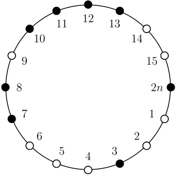
An example of a state (wheren = 8) is shown in figure 1, whereA types are white dots,
and B types are black dots. The figure also shows how locations are numbered.
2n
15 14 13 12 11 10
9
8
7
6
5 4 3
[image:6.595.207.389.275.457.2]2 1
Figure 1: Example of a state with an equal number of black and white dots.
A configuration σ is an assignment of all players to a position on the circle such that no
two players occupy the same position. Given a configuration σ let |Nt
i(σ)| be the number
of players of type t in the neighborhood of li. I sometimes omit σ when there can be no
misunderstanding. Let the set of all possible configurations be Σ.
Preferences Each player cares about her local neighborhood composition. In particular a
player of typet currently residing on locationli gets the following payoff:
ut
i(σ) =
(
0 if |Nit|
3 < 1 2
1 otherwise
Note that the player counts herself in the neighborhood. Let the set of players who have
utility 0 in σ be R(σ)⊆R.
Dynamics Schelling specifies the following adjustment dynamics. Let time be discrete
τ = 0,1,2, . . .. Let the configuration at timeτ be σ(τ). Start with an initial (randomly
specified procedure e.g. pick the player inR(σ(τ)) who has the lowest location number. Let her insert herself at a position in which she gets utility 1, such that she has to travel the
fewest steps from her current position. If the player vacating li inserts herself at position
li′ the new configuration σ(τ + 1) is as follows: if the fewest number of steps from li and
li′ is accomplished by moving counter-clockwise then all players who resided on locations
lj, j = i′, . . . , i−1 are moved one position clockwise so that the new location of a player
who resided at location lj is now lj+1. E.g. the player living on li−1 lives on li in the
new configuration. And equivalently if the fewest number of steps can be accomplished by moving clockwise.
2.2
Analysis
As a first step in the analysis I look for patterns that are stable with respect to the ad-justment process. Then in the next step I establish that from any initial configuration Schelling’s model converges to an element in the set of “stable” configurations.
Stable Configurations I will say that a configurationσ isstableunder Schelling’s
adjust-ment procedure if no player will want to change her location, given her current location and the assignment of the other players to locations on the circle. The following two definitions will be useful for what follows.
Definition 1. A cluster is a contiguous group of at least two players of the same type. A
cluster is minimal if it is of length 2.
Definition 2. A configuration isintegrated if all residents belong to a minimal cluster. A
configuration is segregated if all A players belong to the same cluster.
Throughout I will assume that n is even. This is a necessary condition for integrated
configurations to exist. Note that n even is not required for the characterization of stable
configurations, nor to establish convergence. I now characterize stable configurations:
Proposition 1. A configuration is stable with respect to Schelling’s dynamics if and only
if all players have at least one neighbor of her own type.
Proof. Suppose a player does not have any neighbors of her own type. Since the player can insert herself between any two players, independent of the configuration, she can move to a location where she has at least one neighbor of her own type.
Now suppose all players have at least one neighbor of her own type. Then she gets utility 1 and has no strict incentive to change her location.
Let the set of stable configurations be denoted Σ∗ ⊂Σ.
Remark 1. Note that if n ≥ 4 and even the set of stable configurations contain the fully
integrated configuration, in which all players live in a diverse neighborhood:
· · ·AABBAABB· · ·
and the segregated configuration:
While Schelling conjectured that the dynamic process would converge, Schelling did not provide a proof. I now establish that Schelling’s model with dynamic adjustment converges
to some configuration in Σ∗ starting from any initial configuration, σ(0) ∈Σ.
Definition 3 (Convergence). The process has converged if at any period τ, when players
change locations according the dynamic adjustment process, the following holds:
σ(τ + 1) =σ(τ)
Given a configuration σ, let σ′ be the configuration which is constructed from σ by
moving playeri from location σi to some location l: σ′ =σ(σi,l).
Definition 4 (Pivotal). If for some j ∈Nσi(σ)\ {i} : uj(σ)6=uj(σ
′) then player i is
ex-ante pivotal, P−, for player j. If u
j(σ) = uj(σ′) for all j then she is ex-ante non-pivotal,
P0−.
If for some j ∈Nσi(σ)\ {i}: uj(σ)6= uj(σ
′) then player i is ex-post pivotal, P+, for
player j . If uj(σ) =uj(σ′) for all j then she is ex-post non-pivotal, P0+.
In words, if i is ex-ante pivotal then the utility of at least one of i’s neighbors in σ
changes wheni moves. Ifi isex-post pivotal then the utility of at least one ofi’s neighbors
inσ′ changes afteri’s move.
I now show that Schelling’s dynamic process indeed converges:
Proposition 2. Starting from any initial configurationσ ∈Σthe process converges to some
σ∈Σ∗.
Proof. Suppose σ(τ) is not stable, otherwise we are done. Let the total number of players
who receive utility 0 at timeτ bem(τ). For any configuration we must have 0≤m(τ)≤2n.
Let one of these players be i. i lives on locationσi. i only has neighbors of the other type.
Let her move to the location nearest to σi such that she has utility 1. Such a position must
exist since n > 1, denote it li. By the rule of movement by inserting herself at li she now
has one neighbor of each type. Let this new configuration beσ′ =σ
(σi,li).
iis either P+ (for the player of her own type) orP+
0 . IfiisP+ forj ∈Nli(σ
′)\ {i}then
the utility ofj is now 1. i is either P− (for either both or one of her neighbors) or P−
0 . If i
is P− for some j ∈ N
σi(σ)\ {i} then the utility of j is now 1. Hence the lower and upper
bound on the number of players with utility 0 in the next period, m(τ+ 1), is:
m(τ)−4≤m(τ + 1)≤m(τ)−1
The process converges if for any τ: m(τ) = 0. Thus after at most m(0) steps the process
has converged.
Remark 2. Note that the convergence result does not rely on the order in which players
2.3
Simulations
How does Schelling’s model perform when it is simulated? One of the attractive features of Schelling’s model is that it is extremely easy to do toy simulations. In this section I work out a few simulations by hand in order to get a feel for how the model works, and then in a later present results from numerical simulations.
Eye Balling I first simulate a few randomly drawn starting configurations, and see where
the process ends up. I let n = 10. A dot over a player indicates that they player currently
has utility 0. Recall that the player at the first position has neighbors at position 2 and 20. Each successive line represents one ”dotted” player starting from the left who updates her location.
˙
AB˙ABBAAABBAABB˙ A˙BAABB˙ BAABBAAABBAABBA˙BAABB˙ BAABBAAABBAABBBAAABB
with 4 clusters of each type.
BABB˙ A˙B˙A˙BAAAA˙ BAABB˙ ABB˙ BBBAAB˙A˙BAAAA˙ BAABB˙ ABB˙ BBBAAABBAAAABAABB˙ ABB˙ BBBAAABBAAAAAABBBABB˙ BBBAAABBAAAAAAABBBBB
with 2 clusters of each type.
As can be seen the adaptive process leads to relatively segregated states, but rarely states with full segregation.
Numerical Simulations The numerically simulated model was programmed inFortran
95 (Compaq Visual Fortran v6.6)5. In the actual implementation of the dynamic process
I used the following procedure. For each simulation the starting configuration is drawn as
follows. I make n draws from the set of locations, without replacement, with each location
being equi-probable. Then thenplayers of a particular type are allocated to these locations.
Then players of the other type are then allocated to the remaining available locations. The
dynamic adjustment process is implemented as follows: in each period I find the first player who does not have any neighbors like herself starting from location 1. This player then moves to the location nearest to her current location where she will have at least one player like herself, ending the period. The adjustment process is repeated until all players have at least one neighbor like themselves.
A general issue when performing simulations is the relation between time in the model and time in the real phenomenon which the modeller is trying to capture. Within the present
5
setting, as the number of residents in the model grow, the probability that each resident gets to update her location shrinks at the same rate. In order to avoid this unattractive feature,
when I report simulation results, I scale time by the number of residents (2n), such that a
resident’s probability of updating in any time period is independent of the size of the city. Thus e.g. when I report waiting times they can be thought of in terms of tenant-generations.
Table 1 gives descriptive statistics about the number of moves to convergence starting from a randomly drawn starting configuration. Mean, standard deviation, min and max of the distribution is reported. The number of residents of each type in the simulations
[image:10.595.185.409.250.350.2]n= 10,20,50,100.
Table 1: Convergence Time (Schelling)
Residents of each Type
n 10 20 50 100
Mean .147 .144 .1427 .1404
Std. .0588 .0409 .0259 .0182
Max .4 .325 .26 .215
Min 0 0 .04 .065
Note: 100.000 Observations per column. Time is measured in tenant generations.
It can be seen from the table that convergence is fast. The simulations suggest that the time to convergence is independent of the number of residents.
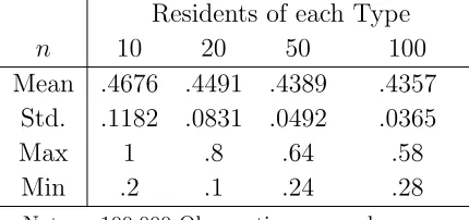
Table 2 shows the mean, standard deviation, the min and max number of clusters for
different sizes of the interacting population. Again the number of residents is varied: n =
10,20,50,100. Note that a configuration with cluster sizek = n
2 is a (fully) integrated stable
configuration, and that a configuration with cluster size equal to 1 is a (fully) segregated
state. Any state with cluster size between k = 1 and k = n
2 is a stable configuration. In
order to facilitate comparison as I vary the number of residents, the number of clusters are
divided through by the maximal number of clusters possible (n/2), which gives us a measure
[image:10.595.189.404.618.719.2]in the range (0,1] independent of the number of residents.
Table 2: Number of Clusters in Stable Configurations (Schelling)
Residents of each Type
n 10 20 50 100
Mean .4676 .4491 .4389 .4357
Std. .1182 .0831 .0492 .0365
Max 1 .8 .64 .58
Min .2 .1 .24 .28
Note: 100.000 Observations per column.
In the following figure the frequency with which some stable configuration withkclusters of each type is selected under the dynamic adjustment process is graphed. It can be seen that the process selects a relative small set of the possible stable neighborhood structures.
0
.2
.4
.6
0
.2
.4
.6
0 10 20 30 0 10 20 30
10 20
50 100
Density
Number of Clusters
[image:11.595.120.478.126.386.2]Graphs by Number of Residents of Each Type
Figure 2: Selection of stable configurations under Schelling’s dynamics. Number of residents
of each type: n= 10,20,50 and 100. 100.000 Observations per graph.
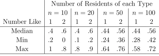
The distribution of clusters in the stable configurations that the process selects for gives a straightforward proxy for how local neighborhoods are composed. Even more informative is the distribution of local neighborhoods. In the next table I report the median fraction of residents who have respectively 1 and 2 neighbors like themselves in their neighborhood across simulations. Note that in any stable configuration all residents must have at least one neighbor like themselves. Also note that in the fully segregated state the fraction of
players with 2 neighbors like themselves is 80%,90%,96% and 98% for n = 10,20,50 and
100 respectively.
Table 3: Composition of local neighborhoods (Schelling)
Number of Residents of each Type
n = 10 n= 20 n= 50 n = 100
Number Like 1 2 1 2 1 2 1 2
Median .4 .6 .4 .6 .44 .56 .44 .56
Min .2 0 .1 .2 .24 .36 .28 .42
Max 1 .8 .8 .9 .64 .76 .58 .72
Note: 100.000 Observations per column.
[image:11.595.159.437.634.733.2]neigh-borhoods only with residents like themselves decrease. The distribution also becomes less dispersed around the median as the number of residents increase.
3
Noise
In this section I ask how noise may help to explain the emergence of segregation. Formally neighborhood evolution is modeled as a Markov process with the current configuration as the relevant state. Noise is then added on top of the deterministic updating process. As the
noise vanishes the process selects states that are stochastically stable (Young 1993)6.
I look at two different variants. First I look at a stochastic variation of Schelling’s model, where the assumption about preferences, made in the previous section, are retained. In order to see how robust analytical results are to other specifications of preference orderings, I also consider a variation where residents have a strict preference for diversity. This second variant also has independent interest. Stable configurations can ranked in terms of aggregate welfare. Then I numerically simulate both models and compare them.
3.1
Noise and Schelling’s Model
In this section I again look at Schelling’s model, but augment with stochastic elements. I assume that players sometimes with small probability make location choices that are unexplained by the model.
3.1.1 Schelling’s Model with Mistakes
Consider the following stochastic version of Schelling’s model.
In each period τ = 0,1,2, . . . a player is randomly selected. All players are equally likely
of being chosen. Suppose playeri at locationli is chosen. ihas the opportunity to move to
a randomly selected locationl (moving either clockwise or counter clockwise), not identical
to her current location, with all locationsl 6=li being equally likely of being chosen.
The probability that player i moves to l depends on the difference between the utility
at her current location and the utility she would get if she moved to l. In particular under
theunperturbed dynamicsimoves with probability one if lstrictly increases her utility, and
remains with probability one otherwise. Under theperturbed dynamics however the resident
sometimes moves (stays) even though staying (moving) gives strictly higher utility. Assume
that there are numbers 0< α < β < γ <∞. For ǫ∈(0, ǫ∗], the decision to remain or move
occur with the following state dependent probabilities:
6
1. If i’s utility increases at l then she moves there with probability
1−ǫα and remains with probabilityǫα.
2. If i is indifferent between her current location andl then she stays
at her current location with probability 1− ǫβ and moves with
probabilityǫβ.
3. If i’s utility decreases at l then she stays at her current location
with probability 1−ǫγ and moves with probability ǫγ.
Note that mistake probabilities are chosen such that the greater the loss in utility from the mistake the less likely the player is to make it. Also note that we have introduced a second stochastic element relative to benchmark: residents no longer moves to the nearest location which is satisfactory, instead they become “aware” of the utility associated with a randomly drawn location.
Model Comments The fact that a resident that moves displaces other residents does not
seem like a realistic assumption about how the residential market works and deserves moti-vation. When a resident moves she simply squeezes in and displaces the original residents. Displacement is also considered by Schelling and Pancs and Vriend.
First, one need not take displacement literally. An alternative interpretation is that there are many more locations than players, and that residents have preferences over the two nearest occupied locations to themselves, e.g. if measured in degrees the set of locations
could be identified with the interval [0,360)⊂R. Second, from a modeling perspective the
assumption ensures that players choice of neighborhood are not constrained by the overall configuration. Thus a particular stable pattern does not come about due to some arbitrary constraints on possible movements. Third, as will be showed this approach yields similar predictions about stable neighborhood structures as do the more realistic assumption of pairs of residents exchanging locations as in Young (1998). Hence, this assumption is not essential for the results.
3.1.2 Analysis
The first result in this section shows that the only recurrent states are the stable configura-tions.
Proposition 3. Under the unperturbed dynamics the set of recurrent states coincides
pre-cisely with the set of stable configurations of Schelling’s deterministic model, Σ∗. Moreover any recurrent state is absorbing.
Proof. The proof can be found in appendix B.1.
Notice that the set of recurrent states coincide with the set of recurrent states in Young (1998). This suggests that the model is robust to the alternative specifications of how players switch places in our two models. I comment on the differences to Pancs and Vriend (2003) in the next section where these differences become even more apparent.
Next I show that the stochastically stable states are precisely the segregated states.
Proof. The proof can be found in Appendix B.2.
The intuition for the result is that it is “easier” (i.e. cheaper in terms of resistance) to reduce the number of clusters than it is to increase it. That is from any initial recurrent state, transitions which reduce the number of clusters are relatively more likely than transitions that increase the number of clusters.
Minimal cost trees are constructed using Lemmas 2 and 3. To get some intuition consider
the simplest case where K = 2. The following picture shows two minimal cost trees, the
first rooted atz1 ∈Z1, i.e. a segregated state, the other rooted atz2 ∈Z2 i.e. an integrated
state.
Z1 Z2
Tree rooted at z1
z1 z′
1 z1′′ z′′
2 z2 z2′
β β
β
β β
Tree rooted at z2
z1 z′
1
z2 z′
2
z′′
1 z′′
2
β γ+β
β
β β
Remark 3. The claim of Proposition 4 holds under the weaker (but less plausible)
as-sumption that mutation rates are independent of the magnitude of utility loss. Suppose that mistakes which leaves the player indifferent or worse off than at her current location both has cost β. Then the claim of Proposition 4 still holds since:
X
k<k′
β > 0
holds for all k′ ≥2.
3.2
Noise and Preferences for Diversity
In the model where residents have threshold preferences, residents are indifferent between living in integrated and segregated local neighborhoods. In this section I assume that players have a strict preference for diversity. I am interested in whether individual incentives to avoid living in a local minority are sufficiently strong to have welfare consequences, that is whether a dynamic process will select equilibria that are relatively or fully segregated.
3.2.1 A Model with Preference for Diversity
I modify the utility function7 to reflect the assumption that players have a strict preference
for diversity.
7
Preferences Given a configuration σ ∈Σ a player of typet who resides on location li has
the following utility function:
ut
i(σ) =
0 if |Nit|
3 ≤ 1 3
1 if 13 < |Nit|
3 ≤ 2 3 x if |Nit|
3 > 2 3
where 12 < x < 1.
That is players value diverse local neighborhoods, but they prefer to live in a ghetto of players like themselves, to living in a ghetto of players who are not like themselves.
Dynamics In each period τ = 0,1,2, . . . one player and a location is chosen at random,
with all players and all locations having positive probability of being chosen. The probability that she moves to the location depends on the utility difference between her current location and the new location.
Specifically let player i, currently living on li, be drawn for location revision and let
l be the location she has the opportunity to move to. Assume that there are numbers:
0< α < β < γ < δ < ψ <∞. For ǫ∈(0, ǫ∗] I assume that the decision to stay at or vacate
li for l is determined by the following procedure:
1. If i’s utility increases at l then she moves there with probability
1−ǫα and remains at l
i with probability ǫα.
2. If i is indifferent between her current location andl then she stays
with probability 1−ǫβ and moves with probability ǫβ.
3. If i currently has utility 1 and l gives utility x then she stays with
probability 1−ǫγ and moves with probability ǫγ.
4. If icurrently has utilityx and l gives utility 0, then she stays with
probability 1−ǫδ and moves with probability ǫδ.
5. If i currently has utility 1 and l gives utility 0 then she stays with
probability 1−ǫψ and moves with probability ǫψ.
3.2.2 Analysis
I begin by characterizing the set of recurrent classes under the unperturbed dynamics,P(0).
Proposition 5. Suppose players have a preference for diversity. Under the unperturbed
dy-namics a configuration is recurrent if and only if each player belongs to a cluster. Moreover:
1. For any σ, σ′ ∈ Σ, σ 6= σ′ such that both have k < K clusters and all players belong to a cluster then σ and σ′ are contained in the same recurrent class.
The set of recurrent states are identical to the set of recurrent states in Young (2001). However in Young’s model all of the recurrent states are also absorbing. The key difference here is that in the present model moves are unilateral, whereas in Young a pair of residents agree to switch places, and this occur only if the joint move is Pareto-improving (“roughly”). Clearly Pareto-improving moves must involve players of different types, but in the present model such switches would involve a player with two neighbors like herself and a player of different type living in a diverse neighborhood.
The contrast with Pancs and Vriend is stark. They assert that “A sufficient condition
[for segregation] on the utility function is that it implies a strict preference for perfect
in-tegration” (Pancs and Vriend 2003, pp. 42-43) this is not the case here. In my set-up if all players strictly prefer integration to being in a minority, and thus to being in a (local) majority, then the only stable outcome is that of perfect integration. This suggest that seg-regation is non-robust to the behavioral assumptions. Specifically our results differ because Pancs and Vriend consider best-replies dynamics, whereas I assume that strategy revision follows better-replies. This is crucial since segregation in Pancs and Vriend is driven by the fact that a perfectly integrated location exists in any configuration (as it does in my set-up). This implies that how players order low ranked neighborhoods is inconsequential. In contrast when players follow better replies this is no longer the case.
Remark 4. Notice that the only absorbing configuration is the integrated state (k = K).
Nevertheless configurations with k < K clusters, and where all players belong to a cluster, are stable in the sense that the process will visit them infinitely often if started in that con-figuration. That is although players have individual micro-incentives to relocate the macro structure is stable.
I now establish that set of segregated states are the only stochastically stable states.
Proposition 6. A state is stochastically stable if and only if it is segregated.
Proof. The proof can be found in Appendix B.4.
The construction of minimal cost trees is shown in the following graph for the case
K = 3. I show the trees for the segregated state and a state with 2 clusters.
Z1 Z2 Z3
Tree rooted at z1
z1 z2
z3 z3′ z3′′
β β β
β
Tree rooted at z2
z1 z2
z3 z3′ z3′′
β β β
3.3
Simulations
3.3.1 Stochastic Version of Schelling
In this section I present numerical simulations of the model for various parameter value of the number of residents and the noise level. The section has two main parts. In the first
part I turn off the noise, i.e. I set ǫ = 0. This allows us to compare how the stochastic
selection procedure affects the convergence time, and clustering in the equilibria selected by the process and compare it to the deterministic version of Schelling. In the second part I examine how the model behaves when there is a positive level of noise.
No Noise Schelling’s model contains two deterministic components that are given
stochas-tic counterparts in our model. First, Schelling assumes that residents who enjoy low utility get to update their choice of location in a deterministic way. In Schelling in each round first all players that have no neighbors like themselves are marked out. Then starting from the right end of the line any player that was marked updates her location, until all marked players have either moved to a new location or they have at least one neighbor like them-selves. After this a new round begins. Second, Schelling assumes that when a player moves she moves to a location closets to her current location where she has at least one neighbor like herself.
In order to see whether the stochastic counterpart of these rules play any role for conver-gence time and the clustering in the equilibria that are reached I simulate the model when
the noise is turned off, i.e. ǫ= 0.
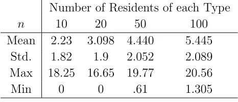
[image:17.595.181.414.473.573.2]The first table shows the convergence time to Nash.
Table 4: Convergence Time (Stochastic Schelling)
Number of Residents of each Type
n 10 20 50 100
Mean 2.23 3.098 4.440 5.445
Std. 1.82 1.9 2.052 2.089
Max 18.25 16.65 19.77 20.56
Min 0 0 .61 1.305
Note: ǫ= 0, 10.000 Observations per column.
Comparing results to Schelling’s original model, convergence is slower for the stochas-tic version. This is not surprising since players who are never selected under Schelling’s procedure is selected for revision in the stochastic version. In particular as the configu-ration comes close to a recurrent state, with only a few players needing to update their locations, the probability that these players are selected decreases in the stochastic version. Thus convergence rates slow down when the configuration gets “close” to a recurrent state. Nevertheless convergence is fairly rapid, and looks roughly linear.
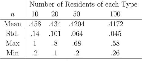
Table 5: Number of Clusters (Stochastic Schelling)
Number of Residents of each Type
n 10 20 50 100
Mean .458 .434 .4204 .4172
Std. .14 .101 .064 .045
Max 1 .8 .68 .58
Min .2 .1 .2 .26
Note: ǫ= 0, 10.000 Observations per column.
Compared to results from simulating Schelling’s original model, the mean number of clusters in the equilibria that are reached under the stochastic version is slightly lower than in Schelling’s model, but more dispersed. The next table confirms that the two models select the same set of equilibria.
Table 6: Composition of local neighborhoods (Stochastic Schelling)
Number of Residents of each Type
n = 10 n= 20 n= 50 n = 100
Number Like 1 2 1 2 1 2 1 2
Median .4 .6 .4 .6 .44 .56 .42 .58
Min .2 0 .1 .2 .2 .32 .26 .42
Max 1 .8 .8 .9 .68 .8 .58 .74
Note: ǫ= 0, 10.000 Observations per column.
I conclude that the stochastic updating and selection of potential allocations does not have a significant impact on the distribution of equilibria that are reached. The only signif-icant impact is on the time to convergence.
In the next part I turn on the noise.
Noise I showed analytically that in the long run the process will only visit the segregated
states. However the result is silent about how long we have to wait before the long run kicks in. In this case simulations are a useful means of examining whether the selection of stochastic stability is economically meaningful. I am interested in how the model behaves with respect to three time aspects of the model: the short, medium and long run.
Definition 5. The short run is the time interval: {0, . . . ,T˜ −1}, where T˜ ≥ 0 is the
random time where the process hits a recurrent class for the first time. The medium run
is the time interval: {T , . . . ,˜ T˜˜}, where T˜˜ ≥ T˜ ≥ 0 is the random time where the process hits an element in the set of stochastically stable states for the first time. The long run is
t:t >T˜˜
For the purpose of the simulations I fix: (α, β, γ) = (1,2,3).8
8
[image:18.595.156.436.347.447.2]The Short Run The following tables show the descriptive statistics of the time of con-vergence to a recurrent class.
Table 7: The Short Run (Stochastic Schelling)
n 10 20 50
ǫ .02 .05 .1 .02 .05 .1 .02 .05 .1
Mean 2.145 2.26 2.455 3.088 3.12 3.395 4.545 4.833 4.895
Std. 1.79 1.80 1.885 1.895 1.925 2.04 2.024 2.241 2.384
Max 12.8 11.4 10.95 11.28 12.68 15.4 15.33 16.77 16.58
Min 0 0 0 .15 .3 .1 1.08 1.10 1.01
Note: (α, β, γ) = (1,2,3), 500 Observations per column.
The Medium Run The following table shows statistics of the duration of the medium
[image:19.595.106.490.378.495.2]run and the fraction of time spent in states that are visited before the process hits one of the stochastically stable states for the first time.
Table 8: Duration of The Medium Run (Stochastic Schelling)
n 10 20 50
ǫ .02 .05 .1 .02 .05 .1 .02 .05 .1
(×103
) (×104
) (×105
)
Mean 6.725 1.07 .024 3.198 .5375 .14 1.688 .265 .0785
Std. 7.40 1.23 .255 2.775 .2075 .1048 1.202 .186 .0575
Max 7.01 7.65 .3825 22.98 2.923 .74 6.037 1.111 .394
Min 0 0 0 .0485 0 .0011 .180 .0225 .0039
Note: (α, β, γ) = (1,2,3), 500 Observations per column.
From the table above it can be seen that the duration of the medium run increases rapidly in the number of residents.
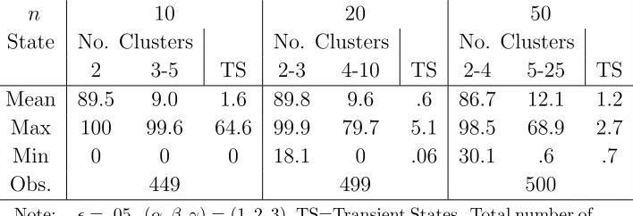
Table 9: Visited States in The Medium Run (Stochastic Schelling)
n 10 20 50
State No. Clusters No. Clusters No. Clusters
2 3-5 TS 2-3 4-10 TS 2-4 5-25 TS
Mean 89.5 9.0 1.6 89.8 9.6 .6 86.7 12.1 1.2
Max 100 99.6 64.6 99.9 79.7 5.1 98.5 68.9 2.7
Min 0 0 0 18.1 0 .06 30.1 .6 .7
Obs. 449 499 500
[image:19.595.122.476.618.739.2]Before transiting to the segregated states the process spends the majority of its time in states which are relatively segregated.
The Long Run The analytical selection result of stochastic stability is a limit result in the
sense that if the noise level goes to zero then the process will spend almost all it’s time in the set of stochastically stable states. In many real life situations factors which are unobserved to the modeler affect the decisions of agents. Therefore we might be unwilling to assume that the noise is vanishing. An alternative is to simulate the model starting from a stochastically stable configuration and then observing the time path of the system for a relatively long period. This allows us to numerically quantify the fraction of time that the process spends in the stochastically stable states. It also provides a way to quantify a threshold for the noise level where the prediction of stochastic stability gives a good approximation of where the system is at any time for a sufficiently long time horizon.
The table below shows the fraction of time spent in various configurations, when the
process is started in a stochastically stable state. I track the process over 107 periods.
Table 10: Fraction of Time Spent in Stochastically Stable States (Schelling)
n 10 20 50
ǫ .02 .05 .1 .02 .05 .1 .02 .05 .1
Stochastically Stable States 99.99 99.79 94.9 99.98 89.1 84.7 99.96 55.1 34.3
Other Recurrent States (*) 0 0 3.4 0 10.4 11.4 0 43.6 55.8
Out of Equilibrium .01 .21 1.8 .02 .5 3.9 .04 1.3 9.9
Note: (α, β, γ) = (1,2,3), Number of Periods: 107
. (*) The process only spends time in recurrent states with less than 4 clusters.
It can be seen that the validity of stochastic stability as the prediction of the long run
behavior of the model depends naturally on ǫ but also on the number of residents. In fact
for ǫ =.1 and n = 50 the process spends a larger fraction of time in recurrent states with
cluster size 2 (39.3%) than it does in the stochastically stable states.
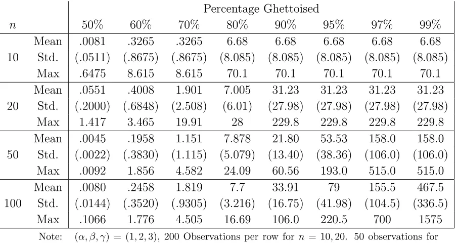
Fist Hitting Times How long does it take forx% of the population to become ghettoized?
The following table answers this question. The table records the mean first hitting time
for x% of the population to only have neighbors like themselves. Standard deviations are
Table 11: First Hitting Times (×103) (Stochastic Schelling)
Percentage Ghettoised
n 50% 60% 70% 80% 90% 95% 97% 99%
10
Mean .0081 .3265 .3265 6.68 6.68 6.68 6.68 6.68
Std. (.0511) (.8675) (.8675) (8.085) (8.085) (8.085) (8.085) (8.085)
Max .6475 8.615 8.615 70.1 70.1 70.1 70.1 70.1
20
Mean .0551 .4008 1.901 7.005 31.23 31.23 31.23 31.23
Std. (.2000) (.6848) (2.508) (6.01) (27.98) (27.98) (27.98) (27.98)
Max 1.417 3.465 19.91 28 229.8 229.8 229.8 229.8
50
Mean .0045 .1958 1.151 7.878 21.80 53.53 158.0 158.0
Std. (.0022) (.3830) (1.115) (5.079) (13.40) (38.36) (106.0) (106.0)
Max .0092 1.856 4.582 24.09 60.56 193.0 515.0 515.0
100
Mean .0080 .2458 1.819 7.7 33.91 79 155.5 467.5
Std. (.0144) (.3520) (.9305) (3.216) (16.75) (41.98) (104.5) (336.5)
Max .1066 1.776 4.505 16.69 106.0 220.5 700 1575
Note: (α, β, γ) = (1,2,3), 200 Observations per row for n = 10,20. 50 observations for
n= 50,100.
Conditional Waiting Times Do waiting times depend upon where we start? The
fol-lowing table documents waiting times conditional upon the first recurrent class which the process hits. 0 5 10 15 20 0 5 10 15 20 1 2 3 4 5 6 7 8 9 10 11 12 13 15 16 17 18 19 20 21 22 23 24 26 27 1 2 3 4 5 6 7 8 9 10 11 12 13 15 16 17 18 19 20 21 22 23 24 26 27 1 2 3 4 5 6 7 8 9 10 11 12 13 15 16 17 18 19 20 21 22 23 24 26 27 1 2 3 4 5 6 7 8 9 10 11 12 13 15 16 17 18 19 20 21 22 23 24 26 27 10 20 50 100
mean of logwait
Graphs by num
Figure 3: Conditional Mean of Log Waiting times for Stochastic Schelling. Number of
clusters in starting recurrent classes on horizontal, and log time on vertical axis. For n =
[image:21.595.119.475.457.720.2]3.3.2 Preference for Diversity
In this section I present simulation results for the model analysed above. For the purpose of the simulations I have fixed: (α, β, γ, δ, ψ) = (1,2,52,3,4).
I begin by looking at the short run behavior of the model.
The Short Run Table 12 shows the time until the process hits a recurrent class of the
[image:22.595.107.494.214.314.2]unperturbed dynamics for the first time.
Table 12: Time to Convergence - The Short Run (Diversity)
n 10 20 50
ǫ .02 .05 .1 .02 .05 .1 .02 .05 .1
Mean 1.565 1.79 1.725 2.208 2.16 2.473 3.035 3.074 3.368
Std. 1.155 1.295 1.4 1.25 2.26 2.7 1.179 1.177 1.506
Max 7.85 6.45 8.05 7.9 8.175 7.125 8.27 7.53 11.66
Min 0 0 0 .4 .4 .5 .89 .89 .94
Note: (α, β, γ, δ, ψ) = (1,2,52,3,4), 200 Observations per column.
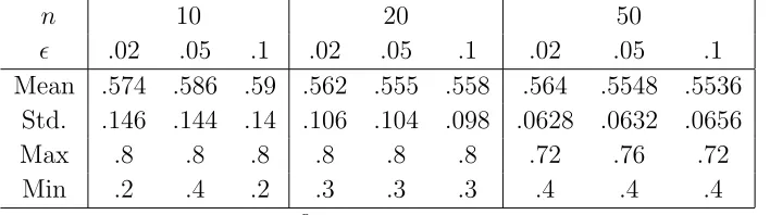
[image:22.595.124.478.439.538.2]The next table details the number of clusters in the configuration when the process hits a recurrent state of the unperturbed dynamics for the first time.
Table 13: Number of Clusters (Diversity)
n 10 20 50
ǫ .02 .05 .1 .02 .05 .1 .02 .05 .1
Mean .574 .586 .59 .562 .555 .558 .564 .5548 .5536
Std. .146 .144 .14 .106 .104 .098 .0628 .0632 .0656
Max .8 .8 .8 .8 .8 .8 .72 .76 .72
Min .2 .4 .2 .3 .3 .3 .4 .4 .4
Note: (α, β, γ, δ, ψ) = (1,2,52,3,4), 200 Observations per column.
I now turn to the medium run.
The Medium Run In the simulations I track the process for a maximum of 107 periods.
The expected wait until the process hits the set of stochastically stable states for the first time is rapidly increasing in the number of residents in the neighborhood. In particular for
n ≥20 the process does not hit the stochastically stable states during the period in which
I track the process. Therefore the medium run behavior of the process, i.e. the states that are visited in the medium run become the most economically interesting time period. Since
the long run is reached within 107 periods for very few observations I report the fraction
Table 14: Visited States in The Medium Run (Diversity)
n 10 20 50
State 2 3-5 OE 2-3 4-5 6-10 OE 2-6 7-12 13-25 OE
Mean 75.40 24.49 .113 10.55 85.64 3.616 .188 0 95.01 4.54 .453
Max 99.96 80.14 .721 18.93 93.67 7.413 .223 0 98.99 10.76 .374
Min 19.69 0 .030 4.030 77.81 .888 .146 0 88.76 .602 .544
Note: ǫ=.05, (α, β, γ, δ, ψ) = (1,2,5
2,3,4), OE=Out of Equilibrium. Forn > 10 the process
does not reach the set of stochastically stable states in 107
periods. Observations per column: 200.
The Long Run In the table below I start the process in the stochastically stable states
and track it for 107 periods. I record the fraction of time which the process spends in the
the different states.
Table 15: Fraction of Time Spent in Stochastically Stable States (Diversity)
n 10 20 50
ǫ .02 .05 .1 .02 .05 .1 .02 .05 .1
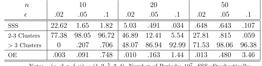
SSS 22.62 1.65 1.82 5.03 .491 .034 .648 .643 .107
2-3 Clusters 77.38 98.05 96.72 46.89 12.41 5.54 27.81 .815 .059
>3 Clusters 0 .207 .706 48.07 86.94 92.99 71.53 98.06 96.38 OE .003 .091 .748 .010 .163 1.44 .013 .480 3.46
Note: (α, β, γ, δ, ψ) = (1,2,5
2,3,4), Number of Periods: 10 7
. SSS=Stochastically Stable States, OE= Out of Equilibrium (transient state).
For reasonable levels of noise stochastic stability is not a valid predictor of where the process will spend most of its time, even for relatively small sizes of the residential neighbor-hood. Compared to the stochastic version of Schelling presented in section 3.1 the process spends much more time in states which are not stochastically stable. This is due to the change in the preferences of residents over local neighborhood composition. In particular in the stochastic version of Schelling if the process is started in a segregated state and a resident by mistake moves to a location with players different from herself then no player like herself has a strict incentive to follow her. On the other hand if residents have a preference for diversity then a mistake opens up a “beachhead” from which a new cluster can form at least temporarily. Since the new cluster is small players from the old cluster is more likely to be drawn for revision and might get the opportunity to move to a diverse neighborhood. Thus the process will spend a significant amount of time outside the segregated state.
Fist Hitting Times How long does it take forx% of the population to become ghettoized.
The following table answers this question. The table records the mean first hitting time
for x% of the population to only have neighbors like themselves. Standard deviations are
reported in parenthesis. I only report figures forn = 10,20,50. As can be seen mean hitting
[image:23.595.82.509.346.455.2]Table 16: First Hitting Times (×104) (Diversity)
Percentage Ghettoised
n 50% 60% 70% 80% 90% 95% 97% 99%
10
Mean .03 .644 .644 31.00 31.00 31.00 31.00 31.00
Std. (.0076) (.9585) (.9585) (28.64) (28.64) (28.64) (28.64) (28.64)
Max .362 4.238 4.238 108.5 108.5 108.5 108.5 108.5
20
Mean .144 .9613 8.47 375.0 - - -
-Std. (.2503) (.9165) (8.03) (40.0) - - -
-Max 1.201 3.278 35.75 199.7 - - -
-50
Mean .1175 1.402 12.60 - - - -
-Std. (.1467) (1.120) (12.80) - - - -
-Max .6566 6.232 57.30 - - - -
-Note: (α, β, γ, δ, ψ) = (1,2,5
2,3,4), 50 observations for each n. Maximum number of
iterations: 109
. “-” indicates that the process did not hit the state within maximum number of iterations.
3.4
Noise and Segregation: Comments
Why do the stochastically stable states not feature prominently within reasonable time frames? The basic intuition is as follows. Suppose the process is started at a state where there are two clusters of each type. The process hits a stochastically stable state when all players are contained on one of the two locations. Due to our assumption about mistake probabilities we need consider only the events where a player moves from one cluster by mistake to the other cluster. Therefore we can approximate the process by a random walk
where the process roughly changes state with probability ǫβ. This base probability has to
be modified by how large the cluster is: residents who live in small clusters are less likely to be drawn for revision than residents who live in a larger cluster. Thus as the size of a cluster shrinks the less likely that a player from that cluster is chosen. This introduces a bias towards clusters of equal size. This behavior of this particular process is hard to characterize analytically, but we can look at a simpler random walk which preserves the main feature that the process is biased towards equal size.
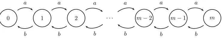
Consider the following random walk on the set of integersZ ={0, . . . , m},m >0. With
probability a the process moves up and with probability b the process moves down, where
a > b > 0 and a+b ≤ 1. Note that the process exhibits a positive drift towards m. The following figure illustrates the process:
0 1 2
a
b
. . . m−2 m−1 m
a
b
a
b
a
b
a
b
a
b
These can be determined from the following recursive relation:
wk = a(wk+1+ 1) +b(wk−1+ 1) + (1−a−b)(wk+ 1)
and the following two boundary conditions:
w0 = 0
wm = b(wm−1+ 1) + (1−b)(wm+ 1)
This is a second order non-homogeneous difference equation with constant coefficients, which can be solved explicitly by standard techniques (see e.g. Sydsaeter and Hammond (1995, p. 750)). Results are summarized in the following Lemma.
Lemma 1. Consider a random walk on the integers between 0 and m. The process moves
up with probability a and moves down with probability b, where a > b > 0 and a+b ≤ 1. The conditional waiting time wk, 0< k≤m, until the process reaches 0 is:
wk =
1− b
a
k
(a−b)(1− b
a) b a
m −
1
a−bk
The waiting time until the process reaches 0 is bounded above by − 1
a−bm+o( a b
m
).
Proof. The proof is in appendix B.5.
For the random walk with drift the waiting time until the process reaches 0 increases
exponentially in m.
Consider a recurrent state of the unperturbed dynamics which contains two clusters of each type. For the purpose of illustrating the connection we need only concern ourselves
with one type of players. Also for small ǫ we need only consider the possibility that β
mistakes occur (recall γ > β thus for small ǫ β-mistakes becomes exponentially more likely
than γ-mistakes. That is the only movements that we need consider is that one player, by
mistake, moves from one cluster to the other cluster. Let the two clusters be denotedcand
˜
crespectively A stochastically stable state is reached whenever say all players from cluster
c has moved to ˜c (or vice versa). All such moves (except the last for r = 1) must occur
via a β mutation. More importantly the process is biased towards selecting some player
from a larger cluster rather than a player from a smaller cluster. To see this note that the
probability that the some player from cluster c is selected equals nc
n, since all players are
equally likely of being drawn for revision, and with remaining probability some player from
cluster ˜cis chosen. Thus as the cluster shrinks the probability that a player from the other
cluster is chosen increases. That is the probability that the cluster grows (via a player from
cluster ˜cmaking a location mistake becomes increasingly higher as the cluster shrinks. Thus
the process is biased towards clusters of equal size. The main simplification is that for the random walk above I have assumed that the bias does not depend upon the state of the walk, whereas in the Schelling model the closer the state moves to 0 the more unlikely is a downward jump and the more likely an upward jump.
increases exponentially in the number of residents. This insight is also applicable to Young’s variants of Schelling.
Why are waiting times even larger when players have a preference for diversity. Consider again as state with two clusters. One minimal cluster and one containing the rest. Since
epsilon is small we can ignore other mistakes apart fromβ mistakes. The waiting time until
the minimal cluster disappears is n222nǫ1β which is the wait until a player from small cluster
is chosen and she draws a location that is diverse in the other cluster times the wait until
she actually makes a β mistake. On the other hand for the minimal cluster to grow, we
just need one of the ghettoized players to be drawn: n−2−2
n−2 and then she must draw an
appropriate location: 2
n so the wait is roughly of order n.
There is a literature on the speed of convergence to the set of stochastically stable states (Young (1998), Ellison (1993, 2000)). The understanding of that literature is that local interaction greatly speeds up convergence to the set of stochastically stable states.
Ellison (1993) and Young (1998, chp. 6) consider local interaction when players play a two person coordination game. Both show that the waiting time until the stochastically stable state is reached is independent of the size of the system. The mechanism through which this is established differ between the two papers.
Ellison (1993) considers an adjustment dynamics a la Kandori, Mailath, and Rob (1993).
That is in each period all players update or adjust their strategy so that their strategy is
a best response to play in the previous period. With small probability players tremble. In each period a player plays a two person coordination game with all the other players. Players may weight payoffs differently from different players. In particular Ellison considers the case where players are located on a circle and a player only assign positive (equal)
weight to her k nearest neighbors on either side. In the k nearest neighbor model for small
enough perturbations the expected waiting time until the process reaches it’s long-run steady state distribution, which puts probability mass one on the risk-dominant equilibrium, is independent of the size of the system. The intuition for the result is as follows. It is already well-known that the risk dominant equilibrium has a larger basin of attraction than the other pure equilibrium. This completely determines what will be selected for in the long run. Now suppose we start the process in the equilibrium which is not risk dominant. In order to transit to the risk dominant equilibrium it is sufficient that a suitable ”small” group of players (who are connected) mutate to the risk dominant strategy. In the next period this will lead their neighbors to switch to the risk dominant strategy as well. The play of the risk dominant strategy then spreads contagiously. Since the basin of attraction of
the risk dominant equilibrium is of larger size, then as ǫ becomes small the risk dominant
equilibrium is selected for.
My version of Schelling’s model contain no contagious element. When play has settled on an equilibrium which is not stochastically stable, all players will have at least one neighbor like themselves. A location mistake (a mutation) will lead at most one other player of the same type to revise her location. This occurs only if the mutating player belongs to a minimal cluster.
most of the time they play a noisy best response. Updates are independently and identi-cally distributed across players. Players interact on a graph, however a given player mainly interacts within relatively small close-knit groups, loosely the group of players that a player interacts with are likely to mainly interact with each other as well. Young asks what the
maximum expected wait until a large proportion 1−p of the population the risk
domi-nant equilibrium, this is called the p-inertia of the process. For sufficiently small mistake
probabilities and if players interact in close-knit groups then the p-inertia of the process is
bounded above, independently of the number of players.
The result relies on the following intuition. First note again that in Young’s model the risk dominant equilibrium is the unique stochastically stable state. Now since all players live in close-knit groups of a given (small) size, starting from the non-risk dominant equilibrium of the coordination game, the wait until a particular group switches to the risk-dominant equilibrium is bounded above, and does not depend on the total number of players in the population. After this event if the probability that players make mistakes is sufficiently small then this group will continue playing the risk dominant for a long time. Since the
process runs simultaneously for all players the waiting time until a large proportion, 1−p,
of the population is playing the risk-dominant equilibrium is bounded.
As is apparent the interaction pattern is substantially different from the current frame-work.
Independent of the underlying preferences the expected wait until the process hits the set of stochastically stable is indeed very long, even for a small number of residents. Stochastic stability is quite uninformative about the behavior of the system for large time periods. Although in both models evolutionary pressures push the process towards segregated states, in the medium run individual preferences over outcomes play a significant role for local neighborhood composition. For the prediction of stochastic stability to be valid the level of noise must be significantly smaller than in the stochastic version of Schelling. This is because starting from a segregated state a location mistake now leads the process directly out of the segregated states, since the location mistake has opened up an opportunity for a player who only lived with players like herself to move to a diverse neighborhood. For a given level of noise it is relatively easier to leave the stochastically stable states.
4
Preference Heterogeneity
In this section I check robustness with respect to preference heterogeneity. I introduce a small portion of players into the population who have different preferences from the majority of the population who have a preference for diversity. These players have preferences of the following form: their most preferred neighborhood is a diverse one, but they prefer living with people different from themselves to only living with people like themselves. One interpretation is that these players are “social activists”, they are willing to live isolated in order to create better outcomes.
is able to push the population towards more integrated outcome? Our simulations suggests that local neighborhoods are remarkably diverse.
4.1
Social Activists
Assume that a small fraction of players are “social activists” in the sense that while their most preferred neighborhood is a diverse one, they prefer to live in isolated neighborhoods
rather than living in ghettos with people like themselves9. That is technically their second
and third ranked alternatives are flipped relative to the remaining population.
This leads to the following formulation of preferences for “social activists”. Given a
configuration σ a social activist of type t residing on location li, has the following utility
function:
vt
i(σ) =
x if |Nit|
3 ≤ 1 3
1 if 13 < |Nit|
3 ≤ 2 3
0 if |Nit|
3 > 2 3
where 12 < x < 1.
I make the additional assumption that all players only care about the type of the players that reside in their local neighborhood, i.e. not whether they are social activists or not.
Apart from this modification the stochastic process is left unchanged.
4.2
Analysis
The next result shows that the presence of just one social activist in a population of players with a preference for diversity has a dramatic effect on long run outcomes. In particular only integrated states are rest points of the unperturbed dynamics.
Proposition 7. Suppose that in a population of players with a preference for diversity there
is at least one social activist. Under the unperturbed dynamics a state is recurrent if and only if it is integrated. Moreover any integrated state is absorbing.
Proof.
⇐: It is immediate that an integrated state is recurrent, since in an integrated state all
players have utility 1, thus no player has strict incentive to move. This shows that an integrated state is absorbing.
⇒: Let a social activist of typet be denoted ts while players with a preference for diversity
are simply denoted by their type, t. We now show that the integrated states are the only
recurrent states. Take any state σ which is not integrated. By the unperturbed dynamics
the process can transit to a state in which all players of typet have at least one neighbour
like themselves. Also by the unperturbed dynamics we can transit to a state where all type
ts players live in a diverse neighbourhood. Let this state be σ′. Suppose σ′ has 1≤k < K
clusters, otherwise we are done.
We now show that we can transit to a state with k+ 1 clusters of each type. Since n
is even and k < K there are at least two players of each type who do not live in diverse
9