ABSTRACT
ZHU, MINYI. Many-body Study of Core-valence Partitioning and Correlation in Systems with Large-Z Element. (Under the direction of Lubos Mitas.)
Quantum Monte Carlo (QMC) is one of the most promising many-body electronic struc-ture approaches in studying strong correlated systems of electrons. We have applied QMC in
the calculation of transition metal oxide and large systems containing heavy elements such as
Thorium and Pb. Relativistic effect becomes non-neglible when heavy elements are involved. However, a direct calculation of relativistic effect in QMC is not practicable because it requires a
4-component framework and all of the electrons need to be considered. Scalar-relativistic
effec-tive core potential(ECP) and 2-component relativistic ECP(RECP) are introudced to quantum chemistry to mimic all-electron calculation including relativistic effects.
We study the accuracy of the ECP of two different sizes of cores by Hartree-Fock, density
functional theory(DFT) and QMC methods using MnO molecule as a test system. We show that the discrepancies between all-electron and ECP calulation of transition metal oxide is actually
caused by the problem of non-linear exchange-correlation functionals in DFT, instead of the
inaccuracy of the ECP. High accuracy diffusion Monte Carlo calculation of the MnO molecule confirms that the Ne-core and He-core ECPs are of comparable quality and therefore enable
to reproduce energy differences within 0.1 eV or better accuracy margin. In addition, we have
corroborated previous results on nodal surfaces which are more most accurate when using trial functions based on orbitals from hybrid functionals.
We make a further modification on the ordinary QMC which extends the applicability to
inherently complex wavefunctions. The complex state can result from a presence of magnetic field, boundary conditions or due to of spin-orbit interactions. The spin-orbit interactions is
particularly interesting since that requires the spin to be dynamic unlike the spin-free mechanism
in ordinary QMC which was restricted to a static label. We implement an inovative spin-sampling technique and fixed-phase approximation for diffusion Monte Carlo(DMC). With the
help of RECP, we calculate the excitation energy of Pb atom and binding properties of Pb
molecules. The excellent agreement with experiment results shows our new spin-orbit QMC is very promising and capable to reproduce spin-orbit interaction.
The study of thorium halides is completed in collaboration with Shi Guo and Shuming Hu. We investigate bond dissociation energies(BDE) of ThXn X=Cl,Br. Comparison of ex-periment results and theoretical calculation including DFT and QMC shows better agreement
when using DMC on ThCln. However, an abnormal experimental BDE curve of ThBrn is not predicted by our calculations which indicates that additional work including both theoretical
Many-body Study of Core-valence Partitioning and Correlation in Systems with Large-Z Element
by Minyi Zhu
A dissertation submitted to the Graduate Faculty of North Carolina State University
in partial fulfillment of the requirements for the Degree of
Doctor of Philosophy
Physics
Raleigh, North Carolina
2013
APPROVED BY:
Celeste Sagui Dean Lee
Elena Jakubikova Lubos Mitas
DEDICATION
BIOGRAPHY
The author was born on April 18, 1985, in Shanghai. He obtained his bachelor degree in Shanghai Jiao Tong University. In 2007, he decided to attend NC State University(NCSU) and started
ACKNOWLEDGEMENTS
I would like to thank my advisor, Lubos Mitas for his help and support. I can not complete my research without his encouragement and advice. His patience, enthusiam and immense
knowledge helped me to accomplish my PhD study. The experience under his guidance will be an invaluable part of my life.
I would like to thank Prof. Celeste Sagui, Prof. Dean Lee and Prof. Elena Jakubikova for
being my committee members and giving me advice on my work. I would also like to thank Department of Physics, NC State University, especially to Prof. Harald Ade and Prof. Chueng
Ji for being the director of graduate programs.
Thank you to all of my past and current group members: Jindrich Kolorenc, Michal Bajdich, Shuming Hu, Xin Li, Rene Derian and Shi Guo. I really enjoy working with my collegues and
they have given me many suggestions on my research, great conversation and great friendship.
TABLE OF CONTENTS
LIST OF TABLES . . . vii
LIST OF FIGURES . . . ix
Chapter 1 Introduction . . . 1
1.1 Organization of This Thesis . . . 1
Chapter 2 Traditional Electronic Structure Theories . . . 3
2.1 Many-body Problem in Electronic Structure Theory . . . 3
2.2 Hartree-Fock Method . . . 4
2.3 Post-Hartree-Fock Method . . . 6
2.4 Density Functional Theory . . . 6
REFERENCES . . . 9
Chapter 3 Quantum Monte Carlo Methods . . . 10
3.1 Introduction . . . 10
3.2 Principle of Monte Carlo Methods . . . 10
3.2.1 Probability Theroy . . . 10
3.2.2 Advantages of Monte Carlo Method . . . 11
3.2.3 Importance Sampling . . . 12
3.2.4 Metropolis Algorithm . . . 14
3.3 Variational Monte Carlo . . . 16
3.4 Variational Trial Wavefunction . . . 17
3.4.1 Cusp Conditions . . . 17
3.4.2 Form of Trial Wavefunction . . . 18
3.5 Optimization of Wavefunction . . . 20
3.5.1 Variance Minimization . . . 20
3.5.2 Energy Minimization . . . 21
3.5.3 Newton Method and Beyond . . . 22
3.6 Diffusion Monte Carlo . . . 23
3.6.1 Time Dependent Green’s Function . . . 23
3.6.2 Short-time Approximation . . . 25
3.6.3 Importance Sampling and Outline of DMC . . . 26
3.6.4 Fixed-Node Approximation . . . 27
3.7 Summary . . . 29
REFERENCES . . . 30
Chapter 4 Study of Ne-core and He-core Pseudopotential Errors in the MnO Molecule . . . 32
4.1 Introduction . . . 33
4.2.1 Ne-core and He-core ECPs . . . 36
4.2.2 Ansatz for the He-core ECP . . . 36
4.2.3 Optimization of ECP . . . 39
4.2.4 Implementation of ECP in QMC . . . 41
4.3 Results . . . 42
4.4 Conclusion . . . 46
REFERENCES . . . 47
Chapter 5 Calculation of Spin-orbit Interaction in QMC . . . 49
5.1 Introduction . . . 49
5.2 Principles of Relativistic Quantum Chemistry . . . 49
5.3 2-component Relativistic Effective Core Potential (RECP) and SCF Theories . . 52
5.4 Spin-Orbit coupling in Quantum Monte Carlo Calculations . . . 57
5.4.1 Trial Wavefunction ofp2 Configuration . . . 57
5.4.2 Spin-dependent Hamiltonian . . . 61
5.4.3 ECP Operator . . . 63
5.4.4 Fixed-phase Approximation and Diffusion Monte Carlo . . . 65
5.5 Results . . . 67
5.5.1 Atomic Results . . . 67
5.5.2 Molecular Results . . . 72
5.6 Additional Benchmarks on Spin Timestep . . . 74
5.7 Conclusion . . . 75
REFERENCES . . . 76
Chapter 6 Dissociation Energy Study of Thorium Halides . . . 78
6.1 Introduction . . . 78
6.2 Computational Methodology . . . 79
6.3 Results . . . 81
6.4 Conclusion . . . 84
REFERENCES . . . 85
Appendices . . . 86
Appendix A Parameters of the He-core ECP for 3d transition-metal elements . . . . 87
Appendix B Parameters of modified Pb RECPs . . . 90
LIST OF TABLES
Table 4.1 The discrepancies between all-electron and Ne-core pseudopotential for the energy difference (eV) between antiferromagnetic and nonmagnetic states
in the MnO solid[2]. . . 34
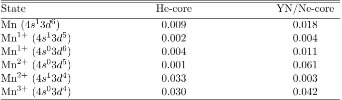
Table 4.2 Parameters of the He-core ECP for Mn, the conventional ECP representa-tion in quantum chemistry programs is used: Vl(r) =r−2PkAklrnkle−Bklr 2 37 Table 4.3 Errors (in eV) of the self-consistent excitation energies of the Mn atom for the two types of ECPs with regard to the all-electron Dirac-Fock calculation 41 Table 4.4 Energy difference ∆ = Ehs −Els between high-spin (2S + 1 = 6) and low-spin (2S + 1 = 2) states of the MnO molecule and corresponding errors quantified as the disagreement between ∆all and ∆ECP for different treatment of the cores and methods. . . 43
Table 4.5 Comparison of QMC excitation energies (eV) and the differences with re-gard to the He-core ECP and differences between the three pseudopoten-tials. In the brackets are types of trial functions which are either single reference built from DFT orbitals or in the last row, multi-reference from CI. . . 45
Table 5.1 Total energy of carbon atom (a.u) . . . 67
Table 5.2 Excitation energies of Pb atom using large core RECP[24] (eV) . . . 70
Table 5.3 Excitation energies of Pb: comparison of large core and small core RECP(eV) 70 Table 5.4 Total energy (atomic unit) of Pb ground state; c: conventional with single vp channel; s: spin sampling, 2-component vpj channels . . . 71
Table 5.5 Excitation energies of Pb atom using conventional and spin sampling QMC (eV) . . . 71
Table 5.6 Dissociation energies of PbH systems using large-core RECP(eV) . . . 73
Table 5.7 Bond lengths(re) and dissociation energies(De) of PbO . . . 74
Table 5.8 DMC total energies of ground state Pb using different spin time step . . . 75
Table 6.1 List of bond lengths[˚A], symmetries, and total energies [a.u.] from DFT(B3LYP) and DMC . . . 81
Table 6.2 Comparison of the BDEs(kcal/mol) of ThBrnfromhybrid-functional DFT(B3LYP) calculation and experiment. The two columns (78e− RECP and 60e− RECP) indicate large-core scalar-relativistic ECP and small-core 2-component relativistic ECP with spin-orbit effect of thorium atom[11]. . . 83
Table A.1 Parameters of the He-core ECP for Sc . . . 87
Table A.2 Parameters of the He-core ECP for Ti . . . 88
Table A.3 Parameters of the He-core ECP for V . . . 88
Table A.4 Parameters of the He-core ECP for Cr . . . 88
Table A.5 Parameters of the He-core ECP for Mn . . . 89
LIST OF FIGURES
Figure 3.1 Target function in the original integral . . . 12 Figure 3.2 Trial distribution in the importance sampling . . . 14 Figure 3.3 Comparison of exact wavefunction Φ0 and fixed-node solution ΦF N in
1-dimension, the error caused by fixed-node approximation is of the order of 5% of correlation energy . . . 28
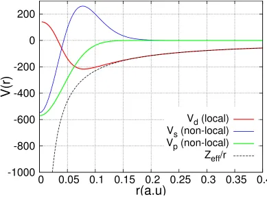
Figure 4.1 He-core pseudopotentials for the Mn atom. . . 38
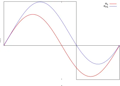
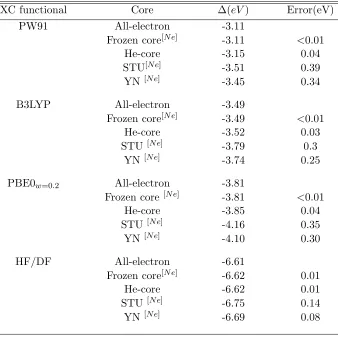
Figure 5.1 Pb atom: 1-component AREP(weighted average of RECP) and 2-component RECP (s, p channels only) [24] . . . 56 Figure 5.2 Energy Levels of group 14 elements. Plotted by I.Kim and Y.S.Lee [31]
using experimental data for C-Pb and theoretical results for Fl . . . 69
Figure 6.1 Experimental bond dissociation energies of Th-F, Th-Cl and Th-Br. Plot-ted by D. L. Hildenbrand and K. H. Lau [3, 4, 5] . . . 80 Figure 6.2 Bond dissociation energies for ThCln molecules. (Data from Shi Guo’s
Chapter 1
Introduction
For several decades, the computational simulation has become an important tool in studying fields of physics, chemistry, material science and bioscience. Theab initiocalculation starts from first principles of quantum mechanics, without implementing any empirical or semi-empirical
parameters in the calculation. With enormous development in the field of high performance computing, first principle methods now enable us to simulate large systems containing hundreds
and thousands of atoms. The electronic structure calculation of atoms, molecules and solids will
help to not only verify but also predict new properties of nanoscale materials.
The main issue of first principle calculation is how to solve the quantum mathematical
equations both efficiently and accurately as Dirac wrote with his famous equation:
“The underlying physical laws necessary for the mathematical theory of a large part
of physics and the whole chemistry are thus completely known, and the difficulty is only that the exact application of these laws leads to equations much too complicated
to be soluble.”
(Post-)Hartree-Fock, density functional theory(DFT), quantum Monte Carlo(QMC),
pseudopo-tential models and many other theories have been successfully developed to solve the
compli-cated equations. The treatment of electron-nucleus, electron-electron interaction and correla-tion is at the heart of these compuacorrela-tion methods. This dissertacorrela-tion will discuss my research
on strongly correlated systems such as transition metal and heavy element systems using high-accuracy quantum Monte Carlo methods and effective core potential models in comparsion with
traditional mean-field approaches.
1.1
Organization of This Thesis
We start by giving a brief introduction to Born-Oppenheimer Approximation, Hartree-Fock,
In Chapter 3, we discuss two typical quantum Monte Carlo methods and concept of
trial-wavefunction.
In Chapter 4, we show the study of ECP’s accuracy by comparing all-electron, He-core and
Ne-core ECPs in DFT, HF and QMC approaches applied to the MnO molecule.
In Chapter 5, we demonstrate the innovative implementation of 2-component REP in QMC which makes it possible to treat spin-orbit interaction in QMC with high accuracy.
Chapter 6 is part of my contribution (collaborated with Hu, Shuming and Guo, Shi) to the
Chapter 2
Traditional Electronic Structure
Theories
For a n-particle system, the exact solution of the many-body Schr¨odinger equations is
pro-hibitively complicated and impossible in most cases. Several popular electronic structure
the-ories and approximations for simplifying non-relativistic many-body problems are briefly re-viewed in this chapter. A comprehensive treatment of relativistic effect is given in Chapter
5.
2.1
Many-body Problem in Electronic Structure Theory
The description of the elctronic structure of matter is derived from the Schr¨odinger equation
in quantum mechanics. The many-body system consists of both heavy nuclei and light electons which interact with each other through the Coulomb interaction. The typical non-relativisic
Hamiltonian for this system is:
ˆ
H =− h
2
2me X
i
∇i2− X
i,I
ZIe2
|ri−RI| +1
2
X
i6=j e2
|ri−rj|
− h
2
2MI X
I
∇I2+ 1 2
X
I,J
ZIZJe2
|RI−RJ|
(2.1)
where mi and MI represent mass of electrons and nuclei, with coordinates ri and RI. Due to the fact that the mass of a nuclei far exceeds the mass of electron, we can assume that the motion(kinetic energy) of the nuclei is negligible compared to that of the electrons. The second
Born-Oppenheimer Approximation. The simplified hamiltonian becomes
ˆ H =−1
2
X
i
∇i2−X i,I
ZIe2
|ri−RI|+
1 2
X
i6=j e2
|ri−rj| (2.2)
where atomic unit is used hereafter. The ith eigenstate Ψi(1,2, . . . , N) of time-independent Schr¨odinger equation
HΨi(1,2, . . . , N) =EΨi(1,2, . . . , N) (2.3) is a many-body wavefunction. The general coordinates (1,2, . . . ,N) include both spin directions
and spatial coordinates. The total energy is the expectation value of the Hamiltonian,
E= hΨ| ˆ H|Ψi
hΨ|Ψi (2.4)
Of particular interest is the ground state of the system, which has the lowest eigenvalues of Eq.2.3. Although the Hamiltonian is simplified by Born-Oppenheimer Approximation, it is still
impractical to get an exact analytical solution to many-body Schr¨odinger equation even for
the system with only a few electrons. A few traditional quantum chemistry methods will be discussed below, in which various further approximations are made.
2.2
Hartree-Fock Method
The early attempt to tackle the many-body problem is known as Hartree product. In 1926, Hartree introduced the theory based on the assumption that each particle is only subjected to
the mean field created by all other electrons. The wavefunction of a non-interacting systems
which is also called Hartree product is given by:
ΨHP(1, . . . , N) =ϕ1(r1)· · ·ϕN(rN) (2.5) However, Hartree equation fails to describe correctly other important properties such as indis-tinguishability of electrons etc. To overcome this problem, Hartree-Fock method was invented
as an extension of Hartree approximation. In Hartree-Fock theory, the motion of each electron
The spin restriction(Pauli principle) forces an antisymmetric form of the wavefunction:
ΨHP(1, . . . , N) = 1 √ N!
ϕ1(r1) ϕ2(r1) · · · ϕN(r1)
ϕ1(r2) ϕ2(r2) · · · ϕN(r2)
..
. ... · · · ... ϕ1(rN) ϕ2(rN) · · · ϕN(rN)
(2.6)
which is written as a normalized slater determinant.
The expectation value of the Hamiltonian is evaluated by
EHF =X si
Z
Ψ ∗
(1, . . . , N)HΨ(1, . . . , N)dr1. . . drN (2.7)
EHF is always greater than or equal to the exact ground state energy. Therefore, the ground state is achieved by so called “Variational principle”. We can use Lagrange’s method of unde-termined multipliers to find the stationary points of the total energy with respect to variations
in the one-particle wavefunctionsδφi. This finally leads to the one-electron Hartree-Fock equa-tions:
−1
2∇
2+V
ion(r) +Vele(r)
φi(r)− X
j δsisj
Z dr0
1
|r−r0|ψ ∗ j(r0)ψ
(
ir 0)∗
ψj(r) =iψi(r) (2.8)
where si is the spin state. Vele represents the Coulomb potential of an electron in the
aver-age charge distribution and the last term on the left side is exchange term that represents
the electron–electron interactions. The advantage of Hartree-Fock theory is that the exchange energy is treated exactly. The Coulomb interaction of an electron with itself (self-interaction
error) gets cancelled by an equivalent term in the exchange part. On the other hand, the
wave-function in general can not be described accurately by just one determinant. The incomplete wavefunction leads to error or so-called correlation energy. Here and in the rest of this thesis,
the electron correlation energy is defined as the difference between Hartree-Fock energy and
the exact energy:
Ecorr =Eexact−EHF (2.9)
2.3
Post-Hartree-Fock Method
Post-Hartree-Fock or sometimes called configuration-interaction(CI) is a many-body ab initio
method in order to recover correlation energy lost in Hartree-Fock approximation. Theoretically, a full CI provides an exact solution of many-body Hamiltonian. The wavefunction is written as
a linear combination of the determinants:
|Ψi=c0|Ψ0i+
X
ar
cra|Ψrai+ X a<b,r<s
crsab|Ψrsabi
+ X
a<b<c r<s<t
crstabc|Ψrstabci+ X a<b<c<d r<s<t<u
crstuabcd|Ψrstuabcdi+· · · (2.10)
where|Ψi is a complete set of determinants including the dominant Hartree-Fock determinant
|Ψ0i, singly excitation |Ψari, doubly excitation |Ψrsabi, etc, up to N-tuply excited determinants. Given N electrons and 2K finite one-electron orbitals (occupied and unoccupied), there exist
2K N
!
different determinants. Therefore even for a small system and moderate number of
one-electron orbitals, the computation cost of full CI is difficult to be fulfilled.
Many practical CI approaches usually limit the length of the CI expansion. For example, in CISD method, only single- and double excitations of the electrons into the virtual orbitals are
considered. But the truncated CI wavefunction probably will not describe e-e correlation
cor-rectly especially for macroscopic systems such as a crystal. In order to simulate solids, millions of determinants are required to construct and be optimized. The lack of size consistency makes
typical CI only appropriate for small molecules with up to 50 electrons(if the quadruple
exci-tations are included) whereas another highly accurate many-body approach–Quantum Monte Carlo method can treat up to 1000 electrons.
2.4
Density Functional Theory
Density functional theory(DFT) is one of the most popular methods for computing properties of solids or super-molecules. The electron density ρ(r) is said to be the probability of finding an electron being present in a certain volume ofdraround the positionr. Mathematically, it is defined as [1]
n(r) =NX s1
· · ·X
sN
Z
dr2· · ·
Z
drN|Ψ(r, s1, r2, s2, . . . , rN, sN)|2 (2.11)
In 1964, Hohenberg and Kohn[2] proposed and proved two simple theorems which makes
DFT possible. The Hohenberg and Kohn theorems demonstrate that for any system of inter-acting particles, the ground state properties are uniquely determined by the density and the
ground state can be achieved by minimizing the functional Etot[n(r)]. The theorems result in the remarkable simplification in which the properties of system depend on only 3 spatial coordinates instead of 3N coordinates.
However, for an exact many-body wavefunction, Eq.2.11 still has infinite terms in the
sum-mation. In 1965, Kohn and Sham[3] made a further approximation and stated that the problem of interacting electrons can be mapped onto solving a fictitious system of non-interacting
“elec-trons”. One-electron orbitals of a non-interacting auxiliary system are introduced from which
the kinetic energy can be computed accurately, leaving only a small correction to be calculated separately. The energy of such a system is expressed as the functional of density:
Etot[n(r)] =− 1 2
N X
i=1
Z
ψ∗i(r)∇2ψi(r) + Z
n(r)Vion(r)dr
+1 2
Z Z
n(r)n(r0)
|r−r0| drdr 0+E
xc[n(r)]
(2.12)
which is composed of the kinetic energy of a non-interacting system, the Coulomb potential, the
Hatree energy and the exchange-correlation energy. The well-known Kohn-Sham equation(an effective one-particle equation) is obtained by minimizing the total energy functional until
self-consistency is achieved:
−1
2∇
2+V
ion[n(r)] +VH[n(r)] +Vxc[n(r)]
ψi(r) =iψi(r) (2.13)
where the Hartree potentialVH is
VH(r) =
Z
dr0 n(r)
|r−r0| (2.14)
and the exchange-correlation potential is
Vxc(r) = δExc[n(r)]
δn(r) (2.15)
All terms in Eq.2.13 are exact and no approximations have been made except the
exchange-correlation potential which is by no means known exactly. One of the most widely used approx-imation to exchange-correlation functional is called the local density approxapprox-imation (LDA).
or a perfect infinite crystal with uniformly distributed valence electrons and positive ions. The
approximation works very well in the case that electron density is almost uniform. But it sur-prisingly also works well for the systems that electron density varies rapidly. QMC played an
important role in finding highly accurate exchange-correlation functional[4].
However, it is common that DFT may get some properties correctly, but fail in predicting others, especially in studying strongly-correlated materials. For example, it is well known that
the LDA and generalized gradient approximation (GGA) predict incorrect equilibrium crystal
structure and electronic state for FeO. In addition, the approximate xc terms leads to a self-interaction error which is very difficult to quantify. To partially remove the impact of this error,
hybrid functional is constructed to incorporate the exact exchange by combining Hartree-Fock
and the density functional treatments of exchange. The most famous hybrid functional are B3LYP[5, 6, 7]:
ExcB3LY P =ExcLDA+a0(ExHF −ExLDA) +ax(ExGGA−ExLDA) +ac(EGGAc −EcLDA) (2.16) and PBE0 functional[8]:
REFERENCES
[1] Parr, Robert G.; Yang, Weitao (1989). Density-Functional Theory of Atoms and Molecules. New York: Oxford University Press.
[2] P. Hohenberg and W. Kohn., Phys. Rev., 136, B864(1964).
[3] W. Kohn and L. J. Sham, Phys. Rev., 140, A1133 (1965).
[4] D. M. Ceperley and B. J. Alder, Phys. Rev. Lett., 45, 566 (1980).
[5] A. D. Becke, J. Chem. Phys., 98, 1372 (1993).
[6] K. Kim and K. D. Jordan J. Phys. Chem., 98,10089 (1994).
[7] P.J. Stephens, F. J. Devlin, C. F. Chabalowski and M. J. Frisch, J. Phys. Chem., 98, 11623 (1994).
Chapter 3
Quantum Monte Carlo Methods
3.1
Introduction
In this chapter, the key idea of the Monte Carlo simulation and its application in many-body quantum mechanics will be discussed. Section 3.1 will review the principle and background of
the Monte Carlo method. Section 3.2–3.5 will introduce several popular implementations of
quantum Monte Carlo in electronic structure calculations.
3.2
Principle of Monte Carlo Methods
3.2.1 Probability Theroy
In mathematics, a probability measure is associated with an event. The probability(p) of the event is defined as the volume of its outcomes (Nk) relative to all possible outcomes(N):
pk= lim
N→∞(Nk/N) (3.1)
A function that maps outcomes of an event in the sample space into a set of real numbers is called random variable. The expectation value of a random variable is defined as
hxi=E(x) =X i
pixi (3.2)
Monte Carlo methods are based on the relation of probability and volume. In fact it uses
the identity of probability in reverse. In Monte Carlo simulation, one draws random samples from a universe of all possible outcomes and interprets the fraction of samples falling into a
given set as the probability. The estimation will converge to the exact value because of the law
The law of large number ensures that the average of independent and identical distributed
( i.i.d.) random variables tend to stabilize at the exact expectation value of the distribution. For example if we draw i.i.d. samplesx1, . . . , xm from a distribution with meanµand variance σ2. Its converge rate is defined by the Central Limit Theorem:
σ2= σ
2
f
m (3.3)
Let’s move forward a small step to integral which is important application of Monte Carlo
A simple integral can be written as
I =
Z b
a
f(x)dx (3.4)
On the other hand, the expectation value of f(x) is
E[f(x)] =
Z b
a
f(x)p(x)dx= lim m→∞
1 m
m X
i=1
f(xi) (3.5)
ifx1, . . . , xmare randomly drawn from a uniform distribution in whichp(xi) = b−a1 . The integral (Eq.3.4) will then be
ˆ
Im = lim m→∞
b−a m
m X
i=1
f(xi) (3.6)
The error of ˆIm−I in the Monte Carlo estimate is a normal distributionN(0,√σf
m).
3.2.2 Advantages of Monte Carlo Method
Many problems in physics involve the calculation of particular integrals (i.e. the Schrodinger
equation). In many cases these integrals are computed by using numerical integration, such
as the Newton-Cotes formulas and the Simpson’s rule. However, traditional numerical integral techniques fail in high dimensional space. Let us consider an integral over a d dimensional hypercube. Using a standard quadrature method such as the trapezoidal rule,with a fixed
spacing of m points per dimension, the error(standard deviation) is proportional to O(m−2/d) toO(m−4/d).
One advantage of Monte Carlo methods over other techniques is the error will still have
the form ofσf/√min all dimensions d. In electronic structure theory, the many-body problem contains N electrons which means 3N dimensional integral. The analytical or numerical solution
becomes intractable. One of the most accurate many-body approaches so far is quantum Monte Carlo method.
target function f(x,y)
-1
-0.5
0
0.5
1 X axis
-1 -0.5
0 0.5
1
Y axis 0
0.2 0.4 0.6 0.8 1
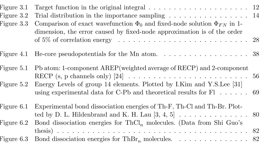
Figure 3.1: Target function in the original integral
not very competitive. However, rather than drawing uniform random points from the space, we
can optimize the simulation by using a better sampling technique such as importance sampling
described as following. The convergence rate will be improved by a significant factor.
3.2.3 Importance Sampling
An example of the efficiency of Monte Carlo simulation is given in Liu’s book[1]. The target function in the example is:
f(x, y) = 0.5e−90(x−0.5)2−45(y+0.1)4 +e−45(x+0.4)2−60(y−0.5)2 (3.7) where (x, y) ∈ [−1,1]×[−1,1], see Figure 3.1. By taking m=1000x1000 uniform grid points in the area of [−1,1]×[−1,1], the integral I = R R
f(x, y)dxdy is evaluated by deterministic algorithm:
ˆ I = 4
m h
f(1)+, . . . , f(m) i
≈
Z Z
f(x, y)dxdy (3.8)
uniformly distributed samples. However, most computation time in the numerical integration
and simple Monte Carlo simulation will be wasted on evaluating the area with zero value. Instead of such unbiased sampling methods, a much more efficient sampling technique will give
more weight to “important” outcomes and is called “importance sampling”. We can write the
integral of interest as
I =
Z
h(x)π(x)dx=Eπ[h(x)] (3.9)
To evaluate this integral, an ordinary Monte Carlo method will draw samplesx1, . . . , xm with probability density functionπ.
ˆ I = 1
m X
i
h(xi) (3.10)
Sampling from π directly is certainly an efficient method. However, in some cases(i.e. a PDE solution), it is impossible to take the samples from π because π distribution has no explicit analytical form. In importance sampling Monte Carlo, we alternatively represent I as
I =
Z
h(x)π(x)
g(x)g(x)dx=Eg
h(x)π(x) g(x)
(3.11)
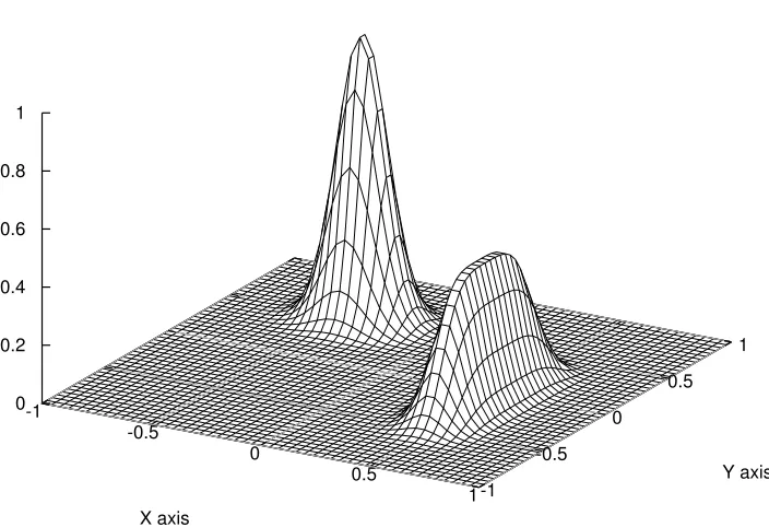
wheregis a nonnegative and normalized probability density function close toπ. The importance sampling drawsx1, . . . , xm from this trial distributiong(Figure 2). The Monte Carlo estimator
with importance sampling associated with g is then given by:
ˆ I = 1
m X
i h(xi)
π(xi)
g(xi) (3.12)
The importance weight π(xi)
g(xi) is a bias correction which can be determined exactly given any
point xi. The key factor of smaller error in estimation lies in selecting an effective importance sampling density g, which should be as ”close” in shape to h(x)π(x) as possible. In an ideal situation,h(x)π(x)/g(x) is a constant for all possiblexi and the importance sampling estimator will have zero-variance. In other cases, the better the approximation is, the smaller variance the estimator will have. In the example, instead of uniform distribution, if we choose a trial
distributiong(x, y) as
g(x, y)∝0.5e−90(x−0.5)2−10(y+0.1)2 +e−45(x+0.4)2−60(y−0.5)2 (3.13) the estimation of the integral I is 0.1259 and the standard error is 0.0005 with sample size m=2500. This is a significant improvement comparing to simple Monte Carlo algorithm in
trial distribution g(x,y)
-1
-0.5
0
0.5
1 X axis
-1 -0.5
0 0.5
1
Y axis 0
0.2 0.4 0.6 0.8 1
Figure 3.2: Trial distribution in the importance sampling
3.2.4 Metropolis Algorithm
The example in the previous example introduces a trial distributiong(x, y) in order to develop an efficient Monte Carlo algorithm. However, the trial distribution in the importance sampling
must be a normalized probability distribution function. Therefore, a normalization constant or a
partition function is required ing(x, y). In general, given any distribution Ψ(X) in configuration space X, the probability density distribution is
P(X) = |Ψ(X)|
2
R
dX|Ψ(X)|2 (3.14)
The partition function R
dX|Ψ(X)|2 is a nontrivial integral which is not easier to solve than the original integral in most cases. To avoid the additional integral, Metropolis algorithm [13]
was developed to draw a collection of samples from any unnormalized distribution function Ψ, which is proportional to the desired probability density ofP.
The Metropolis algorithm is a simulation method based on Markov chains. This algorithm
stateX0, the Metropolis algorithm will be illustrated as the following steps:
1. Propose a trial move from current stateXt toX0.X0. The probability of the transition is defined by a transition probability functionT(Xt, X0). Mathematically, it is a symmetric and ergodic function which satisfies
T(x, y) =T(y, x)
X
yT(x, y) = 1 (3.15)
2. Define the acceptance function A(Xt, X0) as the probability of accepting the trial move. At equilibrium, due to the detailed balance condition[13],A(Xt, X0) can be calculated by:
A(Xt, X0) = min
1,T(X
0, Xt)P(X0) T(Xt, X0)P(Xt)
= min
1,P(X 0) P(Xt)
(3.16)
Obviously, the norm of the target distribution function P got cancelled in the above equation.
3. Generate a random numberu∼Uniform[0,1] and updateX state by
Xt+1 =
(
X0 ifu≤A(Xt, X0)
Xt otherwise (3.17)
Given a variable or operator ˆO, the expectation value is represented by the average of the ensemble at an equilibrium state t.
<O >ˆ N= R
O(Xt)P(Xt)
R
P(Xt)dX ≈ 1 N
N X
i=1
O(Xit) (3.18)
The variance of the measurement is defined as
σ2≈ 1
N −1 N X
i=1
(O(Xit)−<O >ˆ N) (3.19)
3.3
Variational Monte Carlo
We will introduce the first QMC method, variational Monte Carlo(VMC) method in this section.
In QMC, we use the non-relativistic many-body Hamiltonian without mean-field approxima-tions. The kinetic and potential energy operators are given by
T =−1
2 Nele
X
i=1
52i (3.20)
V = Ne X i=1 Nion X A=1 ZA riA + Ne X i=1 Ne X j>i 1 rij (3.21)
VMC is based on the variational principle. Given a trial wavefunction ΨT, the expectation value of Hamiltonian is
ET = hΨT|H|ΨTi
hΨT|ΨTi
=
R
dR|ΨT(R)|2HΨΨT(R)
T(R)
R
dR|ΨT(R)|2 =
R
dR|ΨT(R)|2EL(R) R
dR|ΨT(R)|2
≥E0 (3.22)
where E0 is the exact ground state energy and ET is an upper bound of E0. The component
HΨT(R)
ΨT(R) is called local energyEL. Since|ΨT(R)|
2 is a non negative function and not necessarily
normalized, we can use the importance sampling and the Metropolis algorithm introduced in
the previous section. The trial ground state energy ET is the average of EL
ET = 1 N
N X
i=1
EL(Ri) (3.23)
with estimated variance
σ2E
T = 1 N N X i=1
[EL(Ri)−ET]2 (3.24)
R is a configuration of positions of electrons (r1, r2, . . . , rN). The trial move from R0 to R is realized by a random vector~= (∆r1,∆r2, . . . ,∆rN) which follows Gaussian distribution and
we have
R0 =R+~ (3.25)
individually instead of all together.
If the trial wavefunction ΨT is the exact solution of H,EL is a constant andσE2T = 0 (zero variance). In general, the better ΨT approximation to the ground state wavefunction is, the smaller variance will be. The next section will introduce the variational trial wavefunction used
in our calculations.
3.4
Variational Trial Wavefunction
The form of trial wavefunction is not uniquely determined. Typically, a Hatree-Fock wavefunc-tion or a more generalized multi configurawavefunc-tion CI wavefuncwavefunc-tion multiplied by the Jastrow factor
is the most commonly used trial wavefunction. In VMC, about 50-80% of the correlation energy
can be recovered by using the optimized trial wave functions. Although we have the freedom in choosing the form of wavefunction, wavefunction must satisfy several basic properties. First,
the cusp conditions at the overlap of two particles must be satisfied in order to obtain small
variance of the local energy. Second, the antisymmetric rule of ΨT under the interchange of two electrons is imposed by the property of fermonic system.
3.4.1 Cusp Conditions
The cusp conditions were raised by Kato [3] which ensure that the divergent kinetic energy
and potential cancels each other at the electron-nucleus and electron-electron overlap. With-out the cusp conditions, the local energy Hψ/ψ will be divergent. We first focus on at the electron-nucleus cusp condition. The hydrogen-like Schrodinger equation for single electron can
be presented as
d2 dr2 +
2 r
d dr +
2Z r −
l(l+ 1) r2 + 2E
ψ(r) = 0 (3.26)
where ψ(r) is the radial function of one-electron orbital. All singularity terms r−n must be canceled atriI = 0 and the cusp condition is summarized as :
1 ψ
∂ψ
∂riI =−ZI (3.27)
Similarly, the electron-electron cusp can be derived from a two-body “radial” equation:
"
2 d
2
drij2 + 2 rij
d drij
+ 2
rij
−l(l+ 1)
r2ij + 2E #
ψS(rij) = 0 (3.28)
electron-electron cusp condition: 1 ψS ∂ψS ∂rij = 1
2(l+ 1) (3.29)
For like(parallel) spins, it is,
1 ψS ∂ψS ∂rij = 1 2 (3.30)
and unlike(antiparallel) spins, it is
1 ψS ∂ψS ∂rij = 1 4 (3.31)
3.4.2 Form of Trial Wavefunction
The trial wavefunction in our QMC calculation is represented by the product of antisymmetric
wavefunctions and exponential Jastrow factors (Slater-Jastrow form):
ΨT(R) =ΨA(R) exp [Ucorr(R)] =
Ndet
X
n=1
(dnD↑nD↓n)
×exp
X
iI
χ(riI) +X i6=j
u(rij) + X i6=j,I
w(rij, riI, rjI)
(3.32)
We can write the antisymmetric function in the form of Slater determinants Dn↑ for up spins and Dn↓ for down spins. The determinant is composed of one-electron orbitalsφwhich is taken from (post-)HF or DFT calculation. Assumingφ and ΨT are real functions (we will deal with complex wavefunction in Chapter 5), it is written as the product of radial part and angular part
φk(r,Ω) =Rk(r)Ylkmk(Ω) (3.33)
The radial function is expressed as the expansion of (gaussian) basis sets or numerical
orbitals. The spherical harmonic functionsYlmare complex-valued. In most quantum chemistry packages, a unitary transformation is made in order to use real spherical harmonic functions Slm(In Chapter 5, we will show the equivalent results obtained by using these two approaches):
Sl,m Sl,−m
!
= √1
2
(−1)ml 1
−(−1)ml i !
Yl,m Yl,−m
!
(3.34)
We have already mentioned above that one-particle orbital must satisfy cusp conditions
derivative is zero at riI = 0. However, if we choose proper pseudopotentials (non-divergent at the nucleus), the orbital with zero derivative also satisfies the electron-nucleus cusp. In Chapter 4, a He-core pseudopoential we constructed will be discussed. It is designed for QMC and can
reproduce most all-electron calculation results due to its extremely small core size.
In QMC, The electron-electron cusp condition is fullfilled by the Jastrow factor. In CI cal-culation, the slow convergence of wavefunction is partly resulted from its attempt to reproduce
the correct electron-electron cusp[4]. Therefore, if we make Jastrow parameters satisfy cusp, a
more compact wavefunction could be used in the calculation. This is one of the advantages of QMC over the traditional quantum chemistry methods.
The components of Jastrow factor include one body term χ(riI) for electron-nucleus, two-body termu(rij) for electron-electron and three body termw(rij, riI, rjI) for electron-electron-nucleus. The existence of two-body term favors the global expansion of electron density and
the three-body term contributes to re-adjust the high density area near the nuclei. These
com-ponents are easily expanded in one-dimension basis sets such as:
χ(r) =X k
cenk ak(r) (3.35)
u(r) =X k
ceekbk(r) (3.36)
w(rij, riI, rjI) =X klm
ceenklm[ak(riI)al(rjI) +ak(rjIal(riI)]bm(rij) (3.37)
whose specific forms may vary. The most commonly used Jastrow functions are Pade-Jastrow[5]
and Boys-Handy functions[6] [7]. The basis functions we employed in our program are listed in Ref.[8]:
fcusp(x, γ) =C( x−x
2+x3/3
1 +γ(x−x2+x3/3)−
1
γ+ 3) (3.38)
fpoly−P ade(x, β) = 1−x
2(6−8x+ 3x2)
1 +βx2(6−8x+ 3x2) (3.39)
Using this form of Jastrow factor, we have obtained excellent trial wavefunctions for atomic systems(C–Si)[9][10], molecules [11][12] and solids [13]. In the optimization procedure, the
co-efficients and parameters of these basis functions are optimized to satisfy the cusp conditions
and also make the total energy as low as possible. Furthermore, since electron-electron corre-lation effects are incorporated in the Jastrow functions, it is not necessary to re-optimize the
coefficients of determinants. The correlation energy recovered in QMC depends on the number
our VMC calculation with three-body Jastrow function.
The main purpose of Jastrow factor is to help reduce statistical variance in QMC calculation which will save a large amount of CPU time. Although the Jastrow recovers part of the cusp
conditions, two-body and three-body correlation, it does not change the nodal surface of the
wavefunction. An accurate nodal surface is the key factor of Diffusion Monte Carlo(DMC) calculations. For large systems, multi-determinant wave functions are still necessary to describe
accurate nodal surfaces. We will discuss DMC and its fixed-node approximation in the last
section.
3.5
Optimization of Wavefunction
Typical optimization methods in QMC include variance minimization, energy minimization
and mixture of both. In our calculation, the variational parameters and coefficients in the cusp
(Eq.3.38) and poly-pade functions (Eq.3.39) are optimized while the antisymmetric wavefunc-tions ΨA and configurations are fixed. The observable in VMC is estimated as
hOˆi=
R
dRΨ†T(R) ˆOΨT(R) R
dR|ΨT(R)|2 =hOLiΨ2
T
≡O¯ (3.40)
whereOL=HΨT/ΨT. Variance and energy are the most common observables to be minimized . Gradients (denoted ash·ii) and Hessians (denoted ash·iij) with respect to a set of parameters and coefficients{ci}in Jastrow factors are also calculated so that optimization procedures such as quasi-Newton or Levenberg-Marquardt method can be applied.
3.5.1 Variance Minimization
Although energy minimization is straightforward, variance minimization is more efficient to get an optimized wavefunction[5]. The reason is that variance of the observable is bounded from
below by zero and energy has no lower bounder (the estimation of energy on a finite set is
possible getting lower while the true energy actually increased). The variance of the energy is defined as
σ2c =
R
dRΨ2c(EL−E¯)2
R dRΨ2
c
=h(EL−E¯)2iΨ2
c (3.41)
where c is the set of parameters. The gradient of the variance with respect toci parameter is
(σ2)i = 2
hEL,i(EL−E¯)i+h Ψi
ΨE
2
Li − h Ψi
ΨihE
2
Li −2 ¯Eh Ψi
Ψ(EL− ¯ E)i
Here we take the derivative of each component in Eq.3.41. Since we use the fixed set of
config-urations and correlated sampling as mentioned in [5], the change of Ψ can be ignored,
(σ2)i=2hEL,i(EL−E¯)i
=2h(EL,i−E¯i)(EL−E¯)i (3.43)
Using similar approximation, the gradient of Eq.3.43 is calculated by
(σ2)ij = 2h(EL,i−Ei¯ )(EL,j−E¯)i (3.44) which is a symmetric and positive-definite Hessian matrix.
There are several drawbacks to using variance-minimization in QMC. First, although it
is very efficient in optimizing Jastrow parameters, it becomes less effective in optimizing the determinantal coefficients of the orbitals[14][15][16]. Second, it has been demonstrated that
energy-optimized wavefunctions usually provide better estimates of non-energy-related
observ-ables than variance-optimized ones[17].
3.5.2 Energy Minimization
In this section, we will briefly summarize an energy-minimization method following the approach
of Umrigar and Filippi[16]. The gradient of energy(Eq.3.22) is
¯ Ei =h
Ψi ΨEL+
HΨi Ψ −2 ¯E
Ψi
Ψi (3.45)
=2hΨi
Ψ(EL−E¯)i (3.46)
The expression of gradient(Eq.3.46) which is simplified by Hermicity has zero-fluctuation in
the limit of Ψ being an exact eigenfunction. This is a very important stationary condition for
optimization methods such as Newton method. The straightforward estimator of the energy Hessian is given by
¯ Eij =2
h(Ψij
Ψ +
ΨiΨj
Ψ2 )(EL−E¯)i
− hΨi
ΨiEj¯ − h Ψj
ΨiEi¯ +h Ψi
Umrigar and Fillippi[16] suggested a rearrangement of last term in the Hessian so that the
fluctuation is much less than straightforward Heissian.
¯ Eij =2
h(Ψij
Ψ +
ΨiΨj
Ψ2 )(EL−E¯)i − h
Ψi
ΨiE¯j− h Ψj
ΨiE¯i
+hΨi
ΨEL,ji − h Ψi
ΨEL,ji+h Ψj
ΨEL,ii − h Ψj
ΨEL,ii (3.48)
This symmetric estimator has the same zero-expectation value as Eq.3.47 in the infinite sam-pling but no-zero value and large fluctuation cancelled in finite samsam-pling. As mentioned above,
most of our optimization are performed on Jastrow part only(recent works reveal that non-linear parameters such as the configuration interaction coefficients and orbital parameters can
be optimized by the energy fluctuation potential(EPP) method[18][19]). Therefore a special
rearrangement is applied to Eq.3.48[20][21]
¯ Eij =2
(Ψij
Ψ −
ΨiΨj
Ψ2 )(EL−E¯)
+ 4
(Ψi Ψ − h
Ψi Ψi)(
Ψj Ψ − h
Ψi Ψi)
(EL−E¯)
+hΨi
ΨEL,ji − h Ψi
ΨEL,ji+h Ψj
ΨEL,ii − h Ψj
ΨEL,ii (3.49)
The first line of Eq.3.49 gets cancelled if we only optimize exponential Jastrow parameters. Thus the expensive calculation of Hessian of wavefunction is avoided.
Analytical forms of the first and second derivatives of the energy and variance are given
above. Sometimes the mixture of two schemes yields better trial-wavefunction because it will decrease the fluctuations in the Hessian. The general form of the cost function is then written
as
C(p) =xE¯(p) + (1−x)hσ(p)2i (3.50) where p is the set of parameters to be optimized.
3.5.3 Newton Method and Beyond
Newton methods has been used to find the local minima of cost function for a long time. How-ever, our expressions of the Hessian (Eq.3.44 and Eq.3.49) avoids expensive direct calculations.
In fact, Hessian matrix is obtained from the gradient vectors g instead. The Newton method becomes quasi-Newton method:
1) calculate the (quasi-)Newton direction
∆p=−Hk−1g (3.51)
2) find the step size γ by performing line search and go to a new position
pk+1 =pk+γ∆p (3.52)
3) calculate new gradient gk+1 and Hessian matrix Hk+1. Go back to step 1.
A positive constant adiag is necessary to be adjusted and added to Hessian matrix if it is not positive definite. Other improvement to Newton methods is to combine with the steepest descent method because Newton methods is less effective at the point far from the minimum.
This is so-called Levenberg-Marquardt method[21][22]. When the current position is far from
the minimum, the algorithm behaves like steepest descent; when we are close to the minimum, Newton method will take effect. The new step direction in the parameter space is modified
according to
(Hk+µkI)∆pk=−gk (3.53)
whereI is identity matrices andµ is the positive damping parameter. The above optimization methods are not only applied to QMC calculation, but also implemented in the construction of pseudopotential of transition metal elements(see Chapter 4).
3.6
Diffusion Monte Carlo
Diffusion Monte Carlo (DMC) is developed on the concept of projection and Green’s function formalism in the diffusion process. One of the major advantages of DMC over VMC is that it
projects out the ground state from a set of eigenstates in the trial wavefunction and about 95%
correlation energy can be recovered by DMC.
3.6.1 Time Dependent Green’s Function
The imaginary time many-body Schrodinger equation is given by:
−∂Ψ(R, τ)
∂t =−(H −ET)Ψ(R, τ) (3.54)
where ET is an energy offset and τ is a real variabule under a Wick rotation t→iτ. To solve Ψ(R, τ) by iteration, Eq.3.54 can be transformed into a form of integral
Ψ(R, τ) =
Z
To obtain the expression of Green’s function G(R, τ,R0, τ0), we can operate on both sides of Eq.3.55
(H −ET)Ψ(R, τ0) =
Z
(H −ET)G(R, τ,R0, τ0)Ψ(R, τ)dR0 (3.56) and
− ∂
∂τ0Ψ(R, τ 0) =−
Z
∂G(R, τ,R0, τ0) ∂τ0 Ψ(R
0, τ)dR0 (3.57)
Due of Eq. 3.54, the right sides of Eq.3.56 and Eq.3.57 are equivalent, which leads to a relation
− ∂
∂τG(R, τ,R 0
, τ0) = (H −ET)G(R, τ,R0, τ0) (3.58) There is also an initial condition that implies
G(R, τ,R0, τ) =δ(R−R0) (3.59)
By diffusion algorithm, it follows that
G(R, τ,R0, τ0) =hR|e−(H−ET)(τ−τ0)|R0i
= ∞ X
i
exp(δt(En−ET))φi(R)φi(R0) (3.60)
A complete set of eigenstatesφiis inserted to Eq.3.60. Then rewrite Eq.3.55 for its first iteration
Ψ(R, δt) =
Z ∞ X
i
e−(E−ET)δtφi(R)φi(R0)·X
k
hφk|Ψ(R0,0)idR0
= ∞ X
k=0
hφk|Ψ(R0,0)iφk(R)e−(Ek−ET)δt (3.61)
And for nth iteration, we have
Ψ(R, nδτ) = ∞ X
k=0
hφk|Ψ(R,0)iφk(R) exp[−(Ek−ET)nδτ] (3.62)
In the limit τ → ∞, only the ground state will be projected out from an arbitrary trial wave-function Ψ because all other states are damped exponentially in the evolution as
lim
3.6.2 Short-time Approximation
However, the exact form of Green’s function has yet been solved since neither the eigenstate
nor eigenvalues is known in the function. To obtain the analytic Green’s function, a
short-time approximation is made. We can map the probelm onto solving a diffusion equation. In a short-time approximation, Green’s function is approximated by Trotter-Suzuki formula
hR|exp[−(H−ET)τ]|R0i=hR|exp[−( ˆT+ ˆV −ET)τ]|R0i ≈ hR|e−Tˆe−( ˆV−ET)τ]|R0i
≡Gdif fGB (3.64)
Please note that ˆT and ˆV do not actually commute and the correction is given by
G−Gdif fGB= 1 2[V, T]τ
2+O(τ3) (3.65)
The approximation of Eq.3.64 is only valid for smallτ which makes it called short-time approx-imation. Gdif f and GB are gaussian functions expanding in time. The first term
Gdif f = ( 1 2πτ)
−3N/2exp
−(R−R
0)2
2τ
(3.66)
is a Green’s function which satisfies a diffusion equation in 3N-dimensional space
− ∂
∂τG(R, τ,R
0,0) = 1 2
N X
i=1
∇2iG(R, τ,R0,0) (3.67)
GB is a branching term
GB(R, τ,R0,0) = exp
h
−τ
2(V(R) +V(R 0
)−2ET)
i
(3.68)
which satisfies the rate equation
− ∂
∂τG(R, τ,R
0,0) = (E
3.6.3 Importance Sampling and Outline of DMC
Based on Green’s function Monte Carlo, an improved and more efficient method called diffusion
Monte Carlo is developed to reduce the statistical error during the calculation. The singularity
and significant variance of the potential ˆV in the presence of GB lead to inefficiency of the simple algorithm. In order to reduce the fluctuation in the sampling, we can implement an
importance sampling technique [23][24] with a mixed distributionf(R, τ) = ΨT(R)Ψ(R, τ) in which ΨT is a trial wavefunction.
Rearrange the diffusion equation in terms of f, we find
∂f(R, τ) ∂τ =−
1 2∇
2f(R, τ) +∇ ·[v
D(R)f(R, τ)] + [EL(R)−ET]f(R, τ) (3.70) where the local energy is EL≡HΨ/Ψ andvD =∇ln|ΨT(R)|2 = 2∇ΨT/ΨT. In fact, the new “drift” term “vD” will displace each walker by an additional effective velocity. The new diffusion and branching Green’s functions become
˜
Gdif f = ( 1 2πτ)
−3N/2exp
−(R−R
0−τ v
D(R0))2 2τ
(3.71)
and
˜
GB(R, τ,R0,0) = exp h
−τ
2(EL(R) +EL(R
0)−2E T)
i
(3.72)
The drift velocity inGdif f will drive walkers towards the regions where|Ψ|2 is large. The local energy in GB is used to reduce the fluctuations and avoid singularity from potential V(R ). The transformation also satisfies zero-variance property of importance sampling. When Ψ is the exact wavefunction, EL(R) =E0.
However, the detailed balance condition of Metropolis algorithm is no longer fulfilled because
the Green’s Function with drift term is not symmetric on
˜
Gdif f(R, τ,R0, τ0)= ˜6 Gdif f(R0, τ,R, τ0) (3.73)
In order to achieve the equilibrium, the acceptance of the movement from R’ to R will be
A(R←R0) = min
1, Gdif f(R→R 0)|Ψ
T(R)|2 Gdif f(R←R0)|ΨT(R0)|2
Using the mixed estimator, the DMC energy is estimated as
EDM C = lim τ→∞
he−τ HΨT|H|ΨTi
he−τ HΨ T|ΨTi
= lim τ→∞
R
Ψ∗(R, τ)HΨT(R)dR R
Ψ∗(R, τ)Ψ
T(R)dR
≈ 1
M X
m
EL(Rm) (3.75)
Here Rm is set of samples of electron configurations with importance function f(R, τ) = lim
τ→∞Ψ(R, τ)ΨT(R).
3.6.4 Fixed-Node Approximation
There is a requirement in choosing any function Φ(R) as the distribution of walkers: Φ must be positive everywhere so that it can be interpreted as the probability density function. For bosonic particles, their wavefunction is symmetric under the exchange of any two electrons
ΦB(r1, . . . , ri, . . . , rj, . . . , rN) = ΦB(r1, . . . , rj, . . . , ri, . . . , rN) (3.76)
The symmetric property indicates it is positive all over the space and can be easily used as prob-ability density function. However, the antisymmetric rule for many-fermion systems requires the
change of sign when exchanging two sermonic particles
ΦF(r1, . . . , ri, . . . , rj, . . . , rN) =−ΦF(r1, . . . , rj, . . . , ri, . . . , rN) (3.77)
which means there exists positive and negative regions. Therefore, ΦF can not be used as distribution directly. In order to solve this fermion-sign problem, we represent the wavefunction Φ(R) as the difference of two positive functions: Φ+ and Φ−
ΦF = Φ+−Φ− (3.78)
Φ+ and Φ− are separated by the nodal surface where Φ = 0. They can be imagined as the distribution of walker in positive and negative regions. The nodal structure of a N-particle
system is a 3N −1 dimensional hypersurface since the wavefunction is continuous. Then the problem becomes finding an accurate nodal surface (Φ = 0). But since we do not know the analytical form of exact ground state wavefunction Φ, we will not be able to know the exact
Φ
(r)
r
Φ0
ΦFN
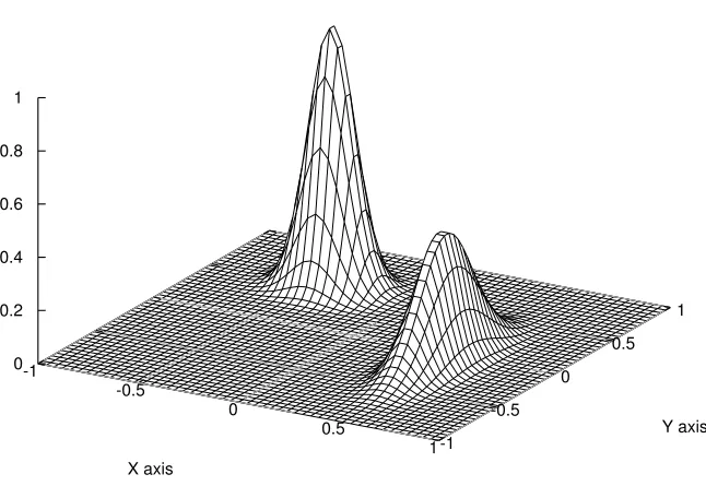
Figure 3.3: Comparison of exact wavefunction Φ0and fixed-node solution ΦF N in 1-dimension, the error caused by fixed-node approximation is of the order of 5% of correlation energy
The practical implementation of the DMC method requires the so-called fixed-node ap-proximation which makes the nodes of the solution ΦF N identical to the nodes of ΨT avoiding thus the fermion sign problem. In an importance sampling DMC formalism, the distribution of
walkers is not the ground state wavefunction Φ but a mixed functionf(R,∞) = Φ(R)ΨT(R). The fixed-node approximation is naturally made by choosing ΨT’s boundary condition as the approximation of exact node. The nonnegative restriction is easily solved so that
f(R, τ)>0 (3.79)
In fact, the drift term vD will push the walker away from the nodes because vD is divergent at f(R) = 0. But it is still possible that the walker can cross the node, although the probability is low. The diffusion vector is proportional to√∆τ. If the drift fails to push away the walker from the nodes because the diffusion move is sufficient large, the walker will cross the nodes and sign
99%. In release-node diffusion Monte Carlo, gaps are opened in the original nodal surface and
walkers can now pass through different nodal pockets[25][26].
In Figure 3, we plot the comparison of an exact wavefunction and fixed-node solution ΦF N in one-dimension. Clearly, there is a fixed-node error in this approximation. The next question is
how fixed-node error affects the result of DMC. It has been shown that fixed-node energy is an upper-bound of the true ground state energy and nodal defect is in the second-order correction
[27] . Furthermore, the fixed-node DMC error is about an order of magnitude smaller than the
VMC error. DMC calculation typically recovers 90–95% of the correlation energy.
Apart from the fixed-node approximation for real wavefunction, it can be extended to
complex-valued wavefunction. We will discuss the fixed-phase approximation in Chapter 5.
3.7
Summary
In this chapter, we have reviewed several applications of Monte Carlo method to quantum
mechanical many-body systems. With modern supercomputers, it is possible to perform QMC calculation on systems up to 1000 particles. On a sufficient large set of samples, VMC is
ca-pable of computing about 80% correlation energy and for DMC, this accuracy could reach
95%. The optimization of Jastrow parameters will reduce the statistical error and save lots of computing time in DMC. Although the most accurate ground state energies can be obtained
by DMC, the nodal surface of trial wavefunction will significantly affect the accuracy. We will
REFERENCES
[1] J. S. Liu, (2001) Monte Carlo Strategies in Scientific Computing Page 31-37, Springer [2] N. Metropolis, A. W. Rosenbluth, M. N. Rosenbluth, A. H. Teller, and E. Teller, J. Chem.
Phys. 21, 1087 (1953)
[3] T. Kato. Commun. Pure Appl. Math, 10, 151 (1957)
[4] B. Klahn and J.D. Morgan III, J. Chem. Phys. 81, 410 (1984).
[5] C. J. Umrigar , K. G. Wilson and J. W. Wilkins , Phys. Rev. Lett. 60, 1719 (1988)
[6] K. E. Schmidt and J. W. Moskowitz, J. Chem. Phys. 97 3382 (1992)
[7] P. J. Reynolds, D. M. Ceperley, B. J. Alder and W. A. Lester, Jr, J. Chem. Phys. 77 5593 (1982)
[8] Michal Bajdich thesisGeneralized Pairing Wave Functions and Nodal Properties for Elec-tronic Structure Quantum Monte Carlo, Appendix A, NCSU, March 2007
[9] Kevin Rasch, Shuming Hu and Lubos Mitas, Unpublished.
[10] K.M.Rasch and L.Mitas, Chemical Physics Letter, 525, 59, (2012)
[11] Shi Guo, Michal Bajdich, Lubos Mitas, Peter J. Reynolds, arXiv:1301.1723 (2013)
[12] Minyi Zhu and Lubos Mitas, Chemical Physics Letters, 572, 136 (2013)
[13] Jindrich Kolorenc and Lubos Mitas, Physical Review B, 75, 235118 (2007)
[14] C. J. Umrigar and Claudia Filippi, J. Chem. Phys. 105, 213 (1996)
[15] Chien-Jung Huang, C. J. Umrigar, and M. P. Nightingale, J. Chem. Phys. 107, 3007 (1997)
[16] C. J. Umrigar and Claudia Filippi, Phys. Rev. Lett. 94, 150201 (2005)
[17] Martin Snajdr and Stuart M. Rothstein, J. Chem. Phys. 112, 11 (2000)
[18] Friedemann Schautz and Stephen Fahy, J. Chem. Phys. 116, 3533 (2002)
[19] Friedemann Schautz and Claudia Filippi, J. Chem. Phys. 120, 10931 (2004)
[20] Xi Lin, Hongkai Zhang, and Andrew M. Rappe, J. Chem. Phys. 112, 2650 (2000)
[21] Michal Bajdich thesisGeneralized Pairing Wave Functions and Nodal Properties for Elec-tronic Structure Quantum Monte Carlo, Page 27-28, NCSU, March 2007
[23] P. J. Reynolds, D. M. Ceperley, B. J. Alder, and W. A. Lester Jr., J. Chem. Phys. 77, 5593 (1982)
[24] R. C. Grimm and R. G. Storer, Journal of Computational Physics 7, 134 (1971).
[25] D. M. Ceperley and B. J. Alder., Phys. Rev. Lett., 45, 566 (1980)
[26] Xin Li, Jindrich Kolorenc and Lubos Mitas, Physical Review A , 84, 023615 (2011)
Chapter 4
Study of Ne-core and He-core
Pseudopotential Errors in the MnO
Molecule
sections of this chapter also appeared in
Study of Ne-core and He-core pseudopotential errors in the MnO molecule: Quantum Monte Carlo benchmark
Minyi Zhu, Lubos Mitas
In this chapter, accuracy of effective core potential (ECP) is studied for two sizes of cores
by Density Functional Theory, Hartree-Fock and quantum Monte Carlo (QMC) methods using the MnO molecule as a test system. We compare the energy differences between high-spin and
low-spin states that were previously found to be problematic for transition metal oxide solids
calculations with ECPs. In order to disentangle errors caused by ECPs and by subsequent methods used in calculations, we construct a scalar-relativistic He-core ECP for Mn atom. We
find that within high quality correlated calculations both Ne-core and He-core ECPs provide
energy differences with comparable, high accuracy. The rest of chapter is organized as follows. After the introduction, a brief summary of relevant methodology is presented in Sec. II, including
the construction of the He-core ECP and its implementation in QMC calculations. In Sec. III, we
show the performance of the constructed ECP and primary results of DFT and QMC methods. We then discuss further aspects of ECPs and electronic structure methods for similar systems.
4.1
Introduction
For several decades transition metal oxide systems have been one of the most challenging
focal topics in chemical and condensed matter physics. Mainstream approaches such as density
functional theory (DFT) and Hartree-Fock (HF) have been applied to these systems quite extensively, however, many of obtained results are mixed at best. For example, it is well-known
that traditional DFT approaches underestimate the band gap of transition metal oxides very
significantly and even fail to predict correct ground states such as insulating antiferromagnets for FeO, CoO and other systems.
Several post-DFT approaches, such as hybrid functionals, on site Coulomb repulsion
correc-tion (LDA+U) or GW approximacorrec-tion have been applied in order to better capture the physics of these strongly correlated systems. Performance of some of these approaches for transition
metal oxide systems have been benchmarked for properties such as band structures, equations of
state and magnetic moments, see, for example, Ref. [1]. Although these more advanced DFT ap-proaches showed marked improvements, significant uncertainties are still present, for example,
in the prediction of pressure induced structural phase transitions [1, 2] and other properties. Of
particular interest are, for example, phase transitions related to the collapse of local magnetic moments such as the one observed in MnO [1, 2]. Similar importance of high-spin vs low-spin
state energy differences can be found in physics and chemistry of molecular (nano) systems
with potential use in spintronics or other applications [3, 4].
The electronic structure calculations for transition metal oxides are often carried out with
the frozen core or with effective core potentials (pseudopotentials) (ECPs). It is assumed that such modification of the original Hamiltonian does not affect the valence properties within the
small and the corresponding ECPs are accurate enough. For 3d elements the Ne-core is con-sidered to be deep and compact enough so that ECPs with 3s,3p,3d,4s states in the valence space faithfully capture the essential physics of all valence properties.
Unfortunately, for some approaches the proper treatment of calculations with ECPs is less
straightforward than one would expect and wish. We illustrate this issue by mentioning a few results of our recent study of MnO solid. In Table 4.1 [2] we show errors for the differnce
between the nonmagnetic (NM) and antiferromagnetic (AFM) states of MnO as obtained from
all-electron and ECP calculations.
Although highly accurate small Ne-core pseudopotentials [5, 6] were used, significant
dis-agreements with all-electron calculation were found ranging from +0.57 eV in generalized
gra-dient DFT to -0.55 eV in HF.
In this work we show that these ”pseudopotential errors” originate in biases gen-erated by the application of approximate methods such as DFT or HF to bonded systems. Assuming that the valence space is sufficiently large, the net contribution of the ECPs to such errors is marginal when compared to errors generated by the approximate
ap-proaches applied to many-body systems with bonds. In this work we explicitly demonstrate that
deep cores have much smaller effect on the basic valence properties than the results from such approximate calculations might suggest. The fact that the approximate theories can generate
additional errors for ECP Hamiltonians has been known in the DFT context for a long time. For example, the nonlinear core corrections for the DFT pseudopotentials have been devised
just for this purpose, ie, to remove the differences between all-electron and pseudopotential
cal-culations [8]. This has been originally justified by the DFT pseudopotential construction which is burdened by the nonlinearity of exchange-correlation functionals so that the core-valence
partitioning is difficult when these two densities overlap appreciably [8]. Very recently, these
types of corrections have been suggested not only for transition elements but also forspsystems in order to decrease the related errors [10]. However, the most accurate ECPs are generated
from Dirac-Fock atomic calculations in energy-adjusted framework (ie, by reproducing not only
one-particle norm conserving properties but also excitation energies) and are designed to repro-duce the physical ion in a true ab initio sense, ie, for use in calculations which can reach nearly
exact eigenstates. Therefore any nonlinearity-like corrections are unusable in many-body wave
function methods. Of the key importance is the genuine many-body accuracy of the (effective)
Table 4.1: The discrepancies between all-electron and Ne-core pseudopotential for the energy difference (eV) between antiferromagnetic and nonmagnetic states in the MnO solid[2].
HF B3LYP PW91

![Figure 5.1:Pb atom: 1-component AREP(weighted average of RECP) and 2-component RECP(s, p channels only) [24]](https://thumb-us.123doks.com/thumbv2/123dok_us/1557322.1191244/67.612.98.464.98.608/figure-component-arep-weighted-average-recp-component-channels.webp)
