A unified tabu search algorithm for vehicle routing problems with soft time windows

(1)

www.palgrave-journals.com/jors

A unified tabu search algorithm for vehicle routing

problems with soft time windows

Z Fu1∗, R Eglese2and LYO Li3

1_{Central South University, Changsha, P.R. China;}2_{Lancaster University Management School, Lancaster,} UK; and3The Hong Kong Polytechnic University, Hong Kong, P.R. China

The different ways of allowing time window violations lead to different types of the vehicle routing problems with soft time windows (VRPSTW). In this paper, different types of VRPSTW are analysed. A unified penalty function and a unified tabu search algorithm for the main types of VRPSTW are presented, with which different types of VRPSTW can be solved by simply changing the values of corresponding parameters in the penalty function. Computational results on benchmark problems are provided and compared with other methods in the literature. Some best known solutions for the benchmark problems in the literature have been improved with the proposed algorithm.

Journal of the Operational Research Society(2008)59,663 – 673. doi:10.1057/palgrave.jors.2602371 Published online 7 February 2007

Keywords:distribution; vehicle routing; soft time windows; heuristics; tabu search

Introduction

The basic vehicle routing problem (VRP) calls for the determination of a set of minimum-cost routes to be performed by a fleet of vehicles to serve a given set of customers with known demands, where each route originates and terminates at a single depot. The total cost consists of two parts, which are the objectives to be minimized: (1) the total number of routes (vehicles) required to serve all customers and (2) the total vehicle travel distance of all routes. It is assumed that the capital cost of an additional vehicle will always exceed any travelling cost that could be saved by its use. Therefore, the priority is given to the first objective. Each customer must be assigned to only one vehicle and the total demand of all customers assigned to a vehicle does not exceed its capacity. The vehicle routing problem with time windows (VRPTW) is an extension of the basic VRP in which vehicle capacity constraints are imposed and each customer i is associated with a time interval [ai,bi], called a time window, during which service must begin. In any vehicle route, the vehicle may not arrive at customer iafter bi to begin service. If a vehicle arrives before ai, it waits. When the time window requirements are strictly enforced, the problem is also called a VRP with hard time windows (VRPHTW). The problem may arise in a variety of applications, including retail distribution, school bus routing, bank deliveries, mail and newspaper deliv-eries, municipal waste collection, fuel oil delivdeliv-eries, and more.

∗_{Correspondence: Z Fu, School of Traffic and Transportation Engineering,}

Central South University at Railway Campus, Changsha, Hunan 410075, P.R. China.

E-mail: [email protected]

The time windows are designed to handle issues such as availability of personnel to load or unload the vehicle, traffic regulations, and customer preferences. For example, a store may only accept deliveries before it opens for business at 9:00 a.m. For VRPHTW, research has flourished over the last two decades. The interested reader will find excellent surveys in Cordeauet al(2002).

The vehicle routing problem with soft time windows (VRPSTW) is an extension of VRPHTW in which some or all customer time window requirements are not strictly enforced and can be violated by paying appropriate penalties. For each customeri, we can define penalty functions to calculate the penalty payable if the vehicle arrives beforeai or after bi. If a certain customer’s time window cannot be violated, that is, it is hard, the penalty payable to that customer for any violation is set to infinity. In that respect, the VRPHTW is a special case of the VRPSTW in which no violations are allowed. There are many good reasons for allowing the time windows to be soft, as stated in Koskosidis et al (1992), Balakrishnan (1993), Taillardet al(1997), Fagerholt (2001), and Chiang and Russell (2004), including:

(1) Many applications do not require a time window that is precise to exact points of time. Therefore, time windows are usually soft by nature.

(2) It is usually impossible to determine accurate vehicle travel times in practice.

(3) Setting the time windows to be soft may allow significant savings in the number of vehicles required and/or the total vehicle travel distance of all routes to be achieved. (4) The VRPSTW model is more general and includes

(2)

extended to solve the VRPHTW by appropriately raising the penalty coefficients.

(5) VRPSTW can always generate feasible solutions in instances where a hard time window approach would have failed. Problems with hard time windows and a small fleet might not have a solution satisfying all customers. In this case, the VRPSTW model would yield usable solutions where some of the customers would not be serviced within the desired time windows.

(6) The VRPSTW model can be used to find a good trade-off between fleet size and service quality to customers.

Note that the objectives to be minimized for the VRPSTW become three: (1) the total number of routes (vehicles) required to serve all customers, (2) the total penalty of time window violations, and (3) the total vehicle travel distance of all routes.

The VRPSTW has received some attention over the last decade. Koskosidis et al (1992) presented an optimization-based heuristic to solve the problem. Balakrishnan (1993) described three simple heuristics for the VRPSTW, which were based on nearest neighbour, Clarke–Wright savings, and space-time rules, respectively. Besides these classical heuris-tics, Taillardet al(1997) designed a tabu search (TS) heuristic for a special case of the VRPSTW, in which the total number of vehicles required was given and fixed. This meant that the fleet size was not a decision variable. Therefore, the objective (1) mentioned above did not need to be minimized. Fagerholt (2001) described a real ship scheduling problem with soft time windows and proposed an optimization-based approach based on a set partitioning formulation to solve the problem. Recently, Chiang and Russell (2004) developed a TS solution method for the type of VRPSTW that Balakrishnan (1993) studied.

In this paper, we present a unified penalty function and a unified TS algorithm for the different types of VRPSTW. Experimental results are reported and compared with other approaches.

Notation and problem representation

Let G = (V,E) be a given undirected network, whereV= {0, . . . ,n}is the vertex set andEis the edge set. Vertices i=1, . . . ,n correspond to the customers, whereas vertex 0 corresponds to the depot.

A non-negative cost, ci j, is associated with each edge (i,j) ∈ E and represents the travel time (distance) spent from vertex i to vertex j. If vehicle k travels directly from vertex i to vertex j, then xi j k = 1, otherwise xi j k =0. A complete network is assumed. If any edges between vertices are missing in the original graph, then they are replaced by edges with an artificially high cost.

Each customeri(i=1, . . . ,n)is associated with a known non-negative demand,di, to be delivered or picked up. A set of identical vehicles, each with capacityC, is available at the

depot. To ensure feasibility, we assume thatdiC for each

i=1, . . . ,n. Each vehicle may serve at most one route. Each vehicle route must start and end at the depot.

Furthermore, each customeri(i=1, . . . ,n) is associated with a time window [ai,bi] during which service should ideally begin and a service timesifor unloading or loading the goods. The depot has a service times0=0, and a time window [a0,b0]. Normally, a0=0. The start time of each vehicle route is greater than or equal toa0. Moreover, observe that the time window requirements induce an implicit orientation of each route even if the original matrices are symmetric, and an implicit route length constraint (ie a latest time instant to complete the route) where the maximum route lengthL=b0. Each route length consists of the vehicle travel time, waiting time at some customers, and time to serve all customers on the route. Therefore, the length of routekis

n

i=0 n

j=0

ci jxi j k+

i∈Nk wi+

i∈Nk si

wherewi is the waiting time at customeriand Nkis the set of customers assigned to routek.

In the hard time window case, a vehicle is not allowed to arrive at customeriafterbi to begin service. If a vehicle arrives beforeai, it waits. However, in the soft time window case, each customer time window can be violated by paying an appropriate penalty. Letti denote the arrival time instant at customeri; the penalty payable P(ti) can be represented as a linear function of the amount of time window violation. For customeri, penalty coefficients i andi are defined to denote the penalty payable for each time unit of service begin-ning before ai and after bi, respectively. In practice, these coefficients could represent the costs of lost sales, goodwill, etc, due to the customer inconvenience for not meeting the time windows, and are therefore often called inconvenience costs. It is not necessary for i and i to be equal, or for these penalty coefficients to be equal across customers. For some important customers or customers whose time window requirements are very strict, the value of i and i can be greater, even set to infinity which, in effect, converts this time window to a hard time window.

The different ways of allowing time window violations lead to different types of VRPSTW.

Type 1: If a vehicle arrives beforeai, it waits, as in the hard time window case. But a vehicle is allowed to arrive at customer i after bi to begin service by paying an appropriate penalty, see Figure 1(a). Taillard et al (1997) proposed a TS heuristic for this type of problem.

(3)

ai bi ai bi ai-Pmax-Wmaxai-Pmax ai bi bi+Pmax

a b c

d e f

[image:3.612.119.476.66.170.2]

ai bi bi+Pmax ai-Pmax ai bi bi+Pmax ai-Pmax ai bi bi+Pmax

Figure 1 Main types of VRPSTW. In each diagram, the horizontal axis represents time and the vertical axis represents the penalty cost.

Type 3: Assume the maximum allowable violation of the time windows to bePmax. Then theouter time windowof each customerimay be enlarged to[ai−Pmax,bi+

Pmax]. Furthermore, assume that the maximum waiting time allowed before the outer time window is

Wmax(see Figure 1(c)). This is the type of the prob-lem that Balakrishnan (1993) and Chiang and Russell (2004) studied. Balakrishnan (1993) described three simple heuristics for it. Chiang and Russell (2004) developed a TS solution method for the problem.

Type 4: Based on Type 1, definePmaxas the maximum allow-able lateness at customer locations, see Figure 1(d).

Type 5: Based on Type 2, definePmaxas the maximum allow-able violation of the time windows. Then theouter time windowof each customerimay be enlarged to

[ai−Pmax,bi+Pmax], see Figure 1(e). The time for the start of service at customerimust be within the outer time window[ai−Pmax,bi+Pmax]and prefer-ably within theinner time window[ai,bi]. The case study by Fagerholt (2001) belongs to this type of problem, in which an optimization-based approach based on a set partitioning formulation was proposed to solve the problem.

Type 6: Based on Type 3, remove the limitation of the max-imum allowable waiting timeWmax, see Figure 1(f).

Some other variants can be defined on the base of the above main types of VRPSTW. If we let Emax and Lmaxrepresent the maximum allowable violation of time windows before

ai and after bi, respectively, instead of Pmax, then a unified penalty function for the above main types of VRPSTW can be defined as

P(ti)=                 

∞(infeasible) ifti<ai−Emax−Wmax iEmax ifai−Emax−Wmaxti

<ai−Emax i(ai−ti) ifai−Emaxti<ai

0 ifaitibi

i(ti−bi) ifbi<tibi+Lmax ∞(infeasible) ifti>bi+Lmax

wherei andi are the penalty coefficients.P(ti)can repre-sent the penalty function for different types of VRPSTW

as different values are assigned to Wmax, Emax, and Lmax. WhenWmax= ∞,Emax=0, andLmax= ∞, it is for Type 1. WhenWmax=0, Emax= ∞, andLmax= ∞, it is for Type 2. When 0<WmaxandEmax,Lmax<∞, it is for Type 3. When Wmax= ∞, Emax=0, and 0<Lmax<∞, it is for Type 4. WhenWmax=0, 0<Emax, and Lmax<∞, it is for Type 5. WhenWmax= ∞, 0<Emax, andLmax<∞, it is for Type 6. Furthermore, whenWmax= ∞and Emax=Lmax=0, it is for the VRPHTW.

As mentioned in the Introduction, the VRPSTW has three objectives to be minimized. Wishing to find a good trade-off between cost and service quality to customers, like Balakrishnan (1993), we judge the quality of the solution obtained using the following criteria in decreasing order of importance: (1) the total number of vehicles used, (2) the total deviation of time window to start service, and (3) the total vehicle travel distance. Therefore, a feasible solution with a certain number of vehicles always dominates over any other feasible solutions requiring more vehicles. This in fact introduces a hierarchical objective function: first, minimize objective (1) and then, for the same number of vehicles, minimize objectives (2) and (3). The objective function can be expressed in pre-emptive goal-programming notation as

Minz=P1K+P2  n

i=1

P(ti)+ n

i=0 n

j=0 K

k=1 ci jxi j k

 

whereK represents the total number of vehicles used, and

P1andP2denote priority levels(P1> >P2). Since objective (2), as stated above, is more important than objective (3), then the level of the importance can be adjusted by the penalty (weight) coefficientsi andi.

The tabu search algorithm

(4)

We developed an effective TS heuristic for the open vehicle routing problem (OVRP) in a previous work (Fuet al, 2005, 2006). The full details of the algorithm were given in the referenced paper and so only the outline of the algorithm and the changes that have been made to apply it to the VRPSTW are described here.

Initial solution

An initial solution is required for any TS algorithm to start the local search process. With respect to the TS metaheuristic for the VRP, some researchers, such as Van Breedam (2001) and Brand˜ao (2004), claimed that the performance of the TS heuristic was highly dependent on the quality of the initial solutions. However, in our previous work (Fu et al, 2005), it was shown that the initial solution did not have a large influence on the final solutions in the proposed TS heuristic. In this paper, therefore, the initial solution is generated by building up successive routes where the next customer is chosen at random and added to the end of the route unless this violates the capacity or route length constraints; in that case the route is completed back to the depot and a new route starts.

Neighbourhood structure

Some discussion of different neighbourhood structures for VRP was presented in Fuet al (2005), including proposals from Pureza and Franc¸a (1991), Osman (1993), Gendreauet al

(1994), Duhamelet al(1997), Cordeauet al(2001), Brand˜ao (2004) and Taillardet al(1997).

The TS algorithm presented in this paper uses the same mixed neighbourhood structure as was introduced in Fuet al

(2005), but some necessary modification is made for the VRPSTW where each vehicle route must start and end at the depot. There are four different types of move that may be used in this mixed neighbourhood structure, and the algo-rithm selects a type of move randomly at each iteration. The four different types of move are based on the 2-interchange mechanism, but differ in the details of the moves that are implemented. The four different types of move are referred to as vertex reassignment, vertex swap, 2-opt and ‘tails’ swap. Some of the possible transformations are described in the following paragraphs.

A solution of the problem can be denoted by a permuta-tion (0,i1,i2,i3,0,i4, . . . ,0,in−1,in,0) of (0, . . . ,n). Only 0 is allowed to appear more than once, each time for a new route. The first 0 and the following vertices before the second 0 consist of the first delivery route, the second 0 and the following vertices before the third 0 consist of the second delivery route, and so on. In consideration of feasibility, the first as well as the last item of a solution must be 0. If one 0 is adjacent to another, that means one route contains no customer, so it can be eliminated.

Select two different vertices (customer or depot, within the same route or different ones) randomly. Examples are shown

underlined below. Perform one of the following four moves randomly.

(a) Vertex reassignment: Remove the first selected vertex from its current position on the route and insert it into the position after the second selected vertex, that is,

X1 = (0135604790280) → X2 = (0156047902830), X1=(0135064709280)→X2=(0135647092800). (b) Vertex swap: Exchange the positions of two

selected vertices, that is, X1 = (0135064790280) → X2 = (0135460790280), X1 = (0135604790280) → X2=(0135004796280).

(c) 2-opt: Reverse the order of all elements between two selected vertices like the standard 2-opt move in TSP, if two selected vertices are within the same route, that is, X1=(0135640790280) → X2=(0146530790280),

X1=(0135604790280)→X2=(0135697400280). (d) ‘Tails’ swap: Exchange the ‘tails’ after two selected

vertices (from the selected vertex to the end of the route; both vertices must be customers), if two selected vertices are in different routes, that is,X1=(0135604790280)→

X2=(0137904560280).

The first and the last 0 of a solution are not allowed to be selected and removed during this 2-interchange process. Note that some moves only make small changes to the current solution and carry on the search within a restricted part of the solution space, facilitating the algorithm to converge; some moves make larger changes to the current solution and guide the search to different areas of the solution space.

(a)–(c) are the moves that can possibly reduce the number of routes. The ‘tails’ swap or move (d) was originally intro-duced because of the structure of the OVRP, where we wished to preserve the ‘tails’ or final parts of routes which would typically include customers far from the depot, while allowing the set of customers included in the early part of the route to be changed. However, this type of move has been retained for the VRPSTW since it allows changes while preserving the sequence of customers in the earlier and later parts of routes, a feature that may be beneficial when time window require-ments are an important feature.

To test the influence of the neighbourhood structure and the search strategy on the performance of the algorithm, we compared the following three cases:

(a) Single type of neighbourhood structure (that is, with only one type of move).

(b) Mixed neighbourhood structure with the above four types of move, and performall of the four moves one by one for the selected two different vertices.

(c) Mixed neighbourhood structure with the above four types of move, but performoneof the four moves randomly for the selected two different vertices.

(5)

structure and the search strategy in which the current move is randomly selected among the four moves are adopted in this TS algorithm.

Evaluation of solutions

To facilitate the exploration of the search space, a move is allowed even if it results in an infeasible solution in terms of the vehicle capacity or route length. The extent of infeasibility can be measured by incorporating the vehicle capacity and maximum route length constraints into the objective func-tion by adding a penalty if the constraints are broken. So a solution can be evaluated by the following objective function

Minz=P1K+P2 _n

i=1 P(ti)+

K

k=1 

n i=0

n

j=0

ci jxi j k+ p(Ec(k)+Et(k))     

where Ec(k) and Et(k) are the excess of load and dura-tion in route k, respectively, andp is the infeasible penalty coefficient. Ec(k) and Et(k)are equal to zero for all routes if a solution is feasible. p ∈ [0.00001,200000] is initially equal to 1 and weighted by a self-adjusting parameter: every 10 iterations, it is divided by 2 if all 10 previous solutions were feasible or multiplied by 2 if all were infeasible. This mechanism was also used in Fuet al(2005), and is based on the method used by Gendreauet al(1994) in the Tabu route algorithm for the VRP.

Tabu list and stopping criterion

The tabu list and stopping criterion also follow the method described in Fu et al (2005). The tabu list contains the move attributes of solutions during the last 5–10 (selected randomly) iterations. The search is terminated if either a specified number of iterations have elapsed in total or since the last best solution was found.

TS algorithm

The following variables are used in the description of the TS algorithm:

iter current number of iterations;

max iter maximum number of iterations;

cons iter current number of consecutive iterations without any improvement to the best solu-tion so far;

max cons iter maximum number of consecutive iterations without any improvement to the best solu-tion so far;

cand list current number of candidate moves on the list;

max cand list maximum number of candidate moves on the list.

The unified TS algorithm for VRPSTW is described below. SetWmax,Emax,Lmax,i andi to the corresponding value according to the type of VRPSTW to be solved and the level of importance between objectives (2) and (3).

Generate an initial feasible solution randomly, and set this solution as the current solution and the best solution so far;

Setiterandcons iterto 0;

While(iter max iter) and (cons iter max cons iter)

do Begin

While(cand list max cand list)do

begin

Select two vertices randomly;

Perform one of the four types of neighbourhood move randomly;

Add the solution produced by the selected move to the candidate list;

end;

Select the best solution in the candidate list if it is not tabu, or it produces a solution strictly

better than the best solution so far;

Set the new solution as the current solution, update the tabu list and incrementiter;

If the new solution improves the best solution so far, update the best solution so far, and set

cons iterto 0; Otherwise, incrementcons iter; End.

This style of TS algorithm was found to be effective for the OVRP in Fuet al(2005), which is why it has been used as the basis for solving the VRPSTW in this paper. Its simple but powerful mixed neighbourhood structure and the stochastic elements in the method allow effective diversification within a local search framework.

Computational results and comparison

This unified TS algorithm was coded in Delphi 7.0 and implemented on a Pentium-II PC running on 600 MHz with 184 MB RAM. To show the computational performance of the algorithm, it was tested on the 56 benchmark prob-lems generated by Solomon (1987) (can be downloaded from: http://w.cba.neu.edu/∼msolomon/problems.htm) and the results were compared with others in the literature.

(6)

in problem sets RC1 and RC2. In problem sets R1, C1 and RC1, the time window is narrow at the central depot so that only a few customers can be served on each route. The time window is wider for problem sets R2, C2, and RC2 so that many customers can be visited on each route and only a few vehicles are required.

Our unified TS algorithm for three of the six main types of VRPSTW that were previously defined (Type 1, Type 2, and Type 3) was tested on the benchmark problems in the liter-ature. The best solutions produced by the algorithm during the course of multiple experiments were compared with those produced by other approaches in the literature, using the criteria of judging the quality of the solution in decreasing order of importance: (1) the total number of vehicles used, (2) the total deviation of time window to start service, and (3) the total vehicle travel distance.

The results were produced with the following bounds:

max cand list=350, max cons iter =5000, and max iter =15000.

Comparison of the results on Type 1 of VRPSTW

Taillard et al (1997) designed a TS heuristic for Type 1 of VRPSTW and tested it on the 56 benchmark problems. The results reported were feasible solutions to the VRPHTW in each case, that is, the percentage of non-violated time windows was 100%, and the number of routes was set to the best solution reported in the literature for each problem, not minimized by the algorithm.

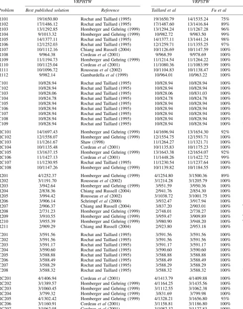
As in Taillardet al(1997), we suppose thati=0,i=100 for alli. The real Euclidean distances between customers are used during the computations, whereas the final results are rounded to the second decimal. The best solutions produced by our unified TS algorithm during the course of multiple experiments are reported in Table 1 for all 56 test prob-lems, using the format: number of routes/total travel distance, percentage of non-violated time windows. In the table, our best solutions are compared with those produced by Taillard

et al(1997) for the VRPSTW and other algorithms reported in the literature for the VRPHTW, respectively, using the format: number of routes/total travel distance. In the table, a double asterisk∗∗indicates that our algorithm has improved the best known solution (lower number of routes required or shorter total travel distance) and a single asterisk∗ means a tie with the best solution produced by Taillardet al(1997). When the percentage of non-violated time windows is 100%, they are compared with those for the VRPHTW as well. An ‘H’ after∗∗ indicates that our algorithm has improved the best published solution and after∗means a tie with the best published solu-tion for the VRPHTW. Overall, our algorithm has improved 25 solutions (12 cases with lower number of routes required, 13 cases with shorter total distance for the same number of routes required and non-violated time windows) and tied 16 solutions on the 56 test problems produced by Taillardet al

(1997) for the VRPSTW, and improved three solutions and

tied 16 best known solutions for the VRPHTW. Note that the method used by Taillard et al (1997) used the best known solution at that time for the number of vehicle routes and did not attempt to minimize the number of routes. The results from our algorithm also show that setting the time windows to be soft does obtain significant savings in the number of vehicles required and/or the total vehicle travelling distance for some routes.

The computation time in seconds for different sets of prob-lems is shown in Table 2.

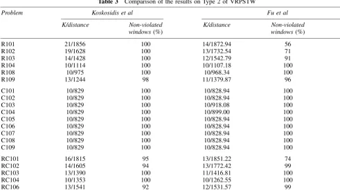
Koskosidis et al (1992) developed an optimization-based heuristic for Type 2 of VRPSTW and tested it on the five sets of randomly generated problems and 21 instances of 56 Solomon’s benchmark problems. The heuristic started with low penalty coefficients, which were gradually increased. In our algorithm, we suppose the penalty coefficients i=i=100 for alliand run it for the 21 instances listed. The comparison of the results is shown in Table 3, using the format: number of routes/total travel distance, percentage of non-violated time windows. The comparison of the CPU time in seconds is in Table 4.

Our algorithm has improved 12 and tied seven solutions on the 21 instances listed, indicated by∗∗and∗, respectively. Among the 12 improved solutions, eight of them require a lower number of vehicle routes and four are of shorter total travel distance (for the same number of routes required and non-violated time windows). For the problem sets of C1, comparing with the heuristic of Koskosidis et al(1992) as well as our algorithm for Type 1 of VRPSTW, our algorithm for Type 2 of VRPSTW takes much more CPU time to find the same best known solutions, and cannot obtain the best known solutions in two instances.

For Type 3 of VRPSTW, Balakrishnan (1993) described three simple heuristics, Chiang and Russell (2004) developed a TS solution method. The eight problems based on the R1 and RC1 sets of the Solomon benchmark problems were used to test the algorithms. The hard time windows in the orig-inal benchmark data were converted to soft time windows by allowing a certain percentage of time window violation,

(7)

[image:7.612.54.545.83.706.2]

Table 1 Comparison of the results on Type 1 of VRPSTW

VRPHTW VRPSTW

Problem Best published solution Reference Taillard et al Fu et al

R101 19/1650.80 Rochat and Taillard (1995) 19/1650.79 14/1535.24 75% ∗∗

R103 13/1292.85 Homberger and Gehring (1999) 13/1294.24 11/1267.28 96% ∗∗

R107 10/1112.16 Chiang and Russell (2004) 10/1126.69 10/1147.59 100%

R108 9/964.38 Cordeauet al(2001) 9/968.59 9/978.69 100%

R109 11/1194.73 Homberger and Gehring (1999) 11/1214.54 11/1264.22 100%

R110 10/1125.04 Cordeauet al(2001) 11/1080.36 11/1083.99 100%

R111 10/1096.72 Rousseauet al(2002) 10/1104.83 10/1138.47 100%

R112 9/982.14 Gambardellaet al(1999) 10/964.01 10/963.22 100% ∗∗

C101 10/828.94 Rochat and Taillard (1995) 10/828.94 10/828.94 100% ∗H

C103 10/828.06 Rochat and Taillard (1995) 10/828.06 10/831.03 100%

RC101 14/1697.43 Homberger and Gehring (1999) 14/1696.94 13/1654.30 92% ∗∗

RC102 12/1558.07 Homberger and Gehring (1999) 12/1554.75 12/1593.71 100%

RC103 11/1261.67 Shaw (1998) 11/1264.27 11/1321.71 100%

RC104 10/1135.48 Cordeauet al(2001) 10/1135.83 10/1175.23 100%

RC106 11/1427.13 Cordeauet al(2001) 11/1448.26 11/1422.72 99%

RC107 11/1230.95 Rochat and Taillard (1995) 11/1230.54 11/1237.64 100%

RC108 10/1147.26 Homberger and Gehring (1999) 10/1139.82 10/1184.55 100%

R202 3/1191.70 Rousseauet al(2002) 3/1214.28 3/1205.79 100% ∗∗

R204 2/838.36 Chiang and Russell (2004) 2/941.76 2/854.30 100% ∗∗

R205 3/994.42 Rousseauet al(2002) 3/1038.72 3/1001.75 100% ∗∗

R206 3/906.14 Schrimpfet al(2000) 3/932.47 3/917.94 100% ∗∗

R207 2/906.37 Chiang and Russell (2004) 3/837.20 2/903.01 100% ∗∗H

R209 3/910.55 Homberger and Gehring (1999) 3/959.47 3/909.89 100% ∗∗H

R210 3/955.39 Homberger and Gehring (1999) 3/980.90 3/948.20 100% ∗∗H

R211 2/909.29 Chiang and Russell (2004) 2/923.80 2/953.18 100%

RC201 4/1406.94 Cordeauet al(2001) 4/1413.79 4/1409.88 100% ∗∗

RC206 3/1160.91 Cordeauet al(2001) 3/1158.81 3/1186.80 100%

RC207 3/1062.05 Cordeauet al(2001) 3/1082.32 3/1127.83 100%

(8)

[image:8.612.48.287.168.252.2]

The computational results of our unified TS algorithm (UTS) and the comparison with the best solution found by Balakrishnan’s simple heuristics (SIM) and Chiang and Russell’s TS with advanced recovery (AR) are presented in Tables 5 and 6. Our algorithm solved all problem instances

Table 2 CPU time on Type 1 of VRPSTW

Problem sets CPU time in second Average

R1 313.08–1203.26 786.34

C1 18.68–238.92 68.41

RC1 190.65–1130.75 697.25

R2 140.77–897.37 528.3

C2 25.37–133.47 56.97

[image:8.612.49.541.301.576.2]

RC2 295.66–882.21 548.73

Problem Koskosidis et al Fu et al

K/distance Non-violated K/distance Non-violated

windows(%) windows(%)

R101 21/1856 100 14/1872.94 56 ∗∗

R102 19/1628 100 13/1732.54 71 ∗∗

R103 14/1428 100 12/1542.79 91 ∗∗

R104 10/1114 100 10/1107.18 100 ∗∗

R108 10/975 100 10/968.34 100 ∗∗

R109 13/1244 98 11/1379.87 96 ∗∗

C101 10/829 100 10/828.94 100 ∗

C102 10/829 100 10/828.94 100 ∗

C103 10/829 100 10/918.08 100

C104 10/829 100 10/899.00 100

C105 10/829 100 10/828.94 100 ∗

C106 10/829 100 10/828.94 100 ∗

C107 10/829 100 10/828.94 100 ∗

C108 10/829 100 10/828.94 100 ∗

C109 10/829 100 10/828.94 100 ∗

RC101 16/1815 95 13/1851.22 74 ∗∗

RC102 14/1605 94 13/1772.42 99 ∗∗

RC103 13/1390 100 11/1416.81 100 ∗∗

RC104 10/1353 100 10/1262.55 100 ∗∗

RC106 13/1541 92 12/1531.57 99 ∗∗

[image:8.612.49.546.625.716.2]

RC108 11/1315 99 11/1224.72 100 ∗∗

Table 4 Comparison of CPU time on Type 2 of VRPSTW

Algorithm Problem sets CPU time in seconds Average Computer

Koskosidiset al R1 209.1–903.3 560.9

C1 2.9–3.3 3.0 IBM3081/VM370

RC1 570.0–834.7 689.4

Fuet al R1 634.8–1357.3 993.1 600 MHz Pentium-II

C1 188.5–472.1 315.1 PC with 184 MB RAM

RC1 453.8–1224.5 810.5

(9)

ZF

u

et

al

—

Ta

bu

search

algorithm

671

Problem Wmax: 0 5 10 0 5

Pmax(Emax, Lmax): 0 0 0 5 5

SIM AR UTS SIM AR UTS SIM AR UTS SIM AR UTS SIM AR UTS

R101 Number of vehicles used 22 19 19 20 19 19 19 16 14 15 17 14 14

Total route distance 2439 2043 1808 1757 1915 1692 1695 1917 1483 1628 1903 1392 1456

% Non-violated windows 100 100 100 100 100 100 100 55 25 42 72 29 37∗

R102 Number of vehicles used 19 19 19 17 17 19 17 17 14 12 12 15 12 12

Total route distance 1958 1685∗∗ 1877 1600 1470∗∗ 1890 1511 1490∗∗ 1754 1364 1389 1693 1259 1348

% Non-violated windows 100 100 100 100 100 100 100 100 69 39 61∗ 80 44 60∗

R103 Number of vehicles used 14 14 13 14 13 14 13 11 11 13 10 11

Total route distance 1475 1381∗∗ 1370 1234 1304 1109 1436 1126 1189 1530 1134 1232

% Non-violated windows 100 100 100 100 100 100 77 60 78∗ 84 60 81

R109 Number of vehicles used 13 12 12 13 12 12 13 12 12 12 11 11 12 11 11

Total route distance 1567 1219 1206∗∗ 1482 1172 1159∗∗ 1492 1165 1158∗∗ 1383 1123 1158 1363 1093 1140

% Non-violated windows 100 100 100 100 100 100 100 100 100 73 62 82∗ 80 58 82∗

Problem Wmax: 10 0 5 10

Pmax(Emax, Lmax): 5 10 10 10

SIM AR UTS SIM AR UTS SIM AR UTS SIM AR UTS

Total route distance 1885 1370 1438 1737 1266 1399 1832 1216 1364 1832 1212 1376

% Non-violated windows 72 24 45∗ 44 14 33∗ 62 11 37∗ 62 8 31∗

% Non-violated windows 83 47 61∗ 63 35 55∗ 78 39 56∗ 81 33 51

% Non-violated windows 86 59 73∗ 68 57 76∗ 82 56 75∗ 83 58 76∗

[image:9.612.77.738.129.474.2]

(10)

Journal

of

the

Operational

Re

search

Society

Vol.

59

,No.

[image:10.612.76.742.125.475.2]

5

Problem Wmax: 0 5 10 0 5

Pmax(Emax,Lmax): 0 0 0 5 5

SIM AR UTS SIM AR UTS SIM AR UTS SIM AR UTS SIM AR UTS

RC101 Number of vehicles used 16 5 16 16 15 15 16 15 15 14 12 13 15 13 13

Total route distance 2200 1764 1913 2012 1643 1704 2012 1651 1685 1835 1522 1594 1972 1425 1554

% Non-violated windows 100 100 100 100 100 100 100 100 100 68 47 72 94 44 72∗

RC102 Number of vehicles used 14 14 14 13 14 14 13 14 13 12 12 14 11 11

Total route distance 1627 1675 1807 1560 1617 1808 1530 1502 1679 1368 1523 1776 1357 1475

% Non-violated windows 100 100 100 100 100 100 100 100 84 60 79∗ 93 61 74∗

RC103 Number of vehicles used 13 11 12 12 11 12 12 11 12 12 10 11 13 10 11

Total route distance 1885 1362 1428 1676 1296 1358 1679 1284 1331 1605 1229 1265 1680 1186 1251

% Non-violated windows 100 100 100 100 100 100 100 100 100 88 79 90 97 69 89

RC106 Number of vehicles used 13 12 13 12 12 12 12 13 11 11 13 11 11

Total route distance 1664 1424 1492 1409 1420 1409 1414 1620 1269 1329 1699 1233 1325

% Non-violated windows 100 100 100 100 100 100 100 95 71 82∗ 98 58 77∗

Problem Wmax: 10 0 5 10

Pmax(Emax,Lmax): 5 10 10 10

SIM AR UTS SIM AR UTS SIM AR UTS SIM AR UTS

RC101 Number of vehicles used 14 13 13 14 11 12 14 11 12 15 11 12

% Non-violated windows 56 39 64∗ 60 25 59 61 36 59 62 27 54

% Non-violated windows 88 58 81 97 55 69∗ 83 56 78∗ 81 56 74∗

% Non-violated windows 82 69 86 92 65 86∗ 92 63 87 83 65 90

(11)

[image:11.612.47.287.76.182.2]

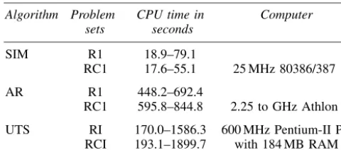
Table 7 Comparison of CPU time on Type 3 of VRPSTW

Algorithm Problem CPU time in Computer

sets seconds

SIM R1 18.9–79.1

RC1 17.6–55.1 25 MHz 80386/387

AR R1 448.2–692.4

RC1 595.8–844.8 2.25 to GHz Athlon

UTS RI 170.0–1586.3 600 MHz Pentium-II PC

RCI 193.1–1899.7 with 184 MB RAM

The computational requirements for TS are greater than the simple heuristics, as shown in Table 7.

Conclusions

The VRPSTW is an extension of the basic VRP and may arise in a variety of applications. The different forms of time window violation allowed lead to different types of VRPSTW. The existing approaches in the literature are usually designed for a special type of VRPSTW. In this paper, the differences and relationships between six main types of VRPSTW are discussed. Then a unified penalty function and a unified TS algorithm for these main types of VRPSTW is proposed, with which a given type of VRPSTW can be solved by simply setting appropriate values for the corresponding parameters in the penalty function. The distinctive features of this TS algo-rithm are the use of a mixed neighbourhood structure based on the 2-interchange generation mechanism, the allowance of the search process to examine solutions that may be infea-sible with respect to the capacity and duration constraints, and the use of stochastic diversification in the selection of the neighbourhood moves and the tabu length. Finally, to test the computational performance of the algorithm, we ran it on the benchmark problems and compared the results with other methods for three types of VRPSTW in the literature. It showed that our algorithm has improved many best known solutions for the benchmark problems.

Acknowledgements—We are grateful to the anonymous referees for their useful comments and suggestions that helped us to improve the presen-tation of this paper. This research was supported by the National Natural Science Foundation of China (NSFC, 70071003, 70671108).

References

Balakrishnan N (1993). Simple heuristic for the vehicle routing problem with soft time windows.J Opl Res Soc44: 279–287. Brand˜ao J (2004). A tabu search algorithm for the open vehicle routing

problem.Eur J Opl Res157: 552–564.

Chiang W-C and Russell RA (2004). A metaheuristic for the vehicle-routing problem with soft time windows. J Opl Res Soc 55: 1298–1310.

Cordeau J-F, Laporte G and Mercier A (2001). A unified tabu search heuristic for vehicle routing problems with time windows.J Opl Res Soc52: 928–936.

Cordeau J-F, Desaulniers G, Desrosiers J, Solomon MM and Soumis F (2002). VRP with time windows. In: Toth P and Vigo D (eds). The Vehicle Routing Problem. SIAM Monographs on Discrete Mathematics and Applications. SIAM: Philadelphia PA, pp 157–194.

Duhamel C, Potvin JY and Rousseau JM (1997). A tabu search heuristic for the vehicle routing problem with backhauls and time windows.Transport Sci31: 49–59.

Fagerholt K (2001). Ship scheduling with soft time windows: An optimisation based approach.Eur J Opl Res131: 559–571. Fu Z, Eglese R and Li LYO (2005). A new tabu search heuristic for

the open vehicle routing problem.J Opl Res Soc56: 267–274. Fu Z, Eglese R and Li LYO (2006). Corrigendum: A new tabu search

heuristic for the open vehicle routing problem.J Opl Res Soc57: 1018–1018.

Gambardella LM, Taillard E and Agazzi G (1999). MACS-VRPTW: A multiple ant colony system for vehicle routing problems with time windows. In: Corne D, Dorigo M and Glover F (eds).New Ideas in Optimization. McGraw-Hill: London, pp 63–76. Gendreau M, Hertz A and Laporte G (1994). A tabu search heuristic

for the vehicle routing problem.Mngt Sci40: 1276–1290. Glover F and Laguna M (1997). Tabu Search. Kluwer Academic

Publishers: Norwell, MA.

Homberger J and Gehring H (1999). Two evolutionary metaheuristics for the vehicle routing problem with time windows.INFOR 37: 297–318.

Koskosidis YA, Powell WB and Solomon MM (1992). An optimization-based heuristic for vehicle routing and scheduling with soft time windows constraints.Transport Sci26: 69–85. Osman IH (1993). Metastrategy simulated annealing and tabu search

algorithms for the vehicle routing problem. Ann Opns Res 41: 421–451.

Pureza VM and Franc¸a PM (1991). Vehicle routing problems via tabu search metaheuristic. Technical Report CRT-347, Centre for Research on Transportation, Montreal, Canada.

Rochat Y and Taillard ED (1995). Probabilistic diversification and intensification in local search for vehicle routing.J Heuristics1: 147–167.

Rousseau LM, Gendreau M and Pesant G (2002). Using constraint-based operators to solve the vehicle routing problem with time windows.J Heuristics1: 43–58.

Schrimpf G, Schneider J, Stamm-Wilbrandt H and Dueck G (2000). Record breaking optimization results using the ruin and recreate principle.J Comput Phys159: 139–171.

Shaw P (1998). Using constraint programming and local search methods to solve vehicle routing problems. In: Maher M and Puget J-F (eds). Principles and Practice of Constraint Programming-CP98, Lecture Notes in Computer Science. Springer-Verlag: New York, pp 417–431.

Solomon MM (1987). Algorithms for the vehicle routing and scheduling problems with time window constraints.Opns Res35: 254–265.

Taillard E, Badeau P, Gendreau M, Guertin F and Potvin JY (1997). A tabu search heuristic for the vehicle routing problem with soft time windows.Transport Sci31: 170–186.

Van Breedam A (2001). Comparing descent heuristics and metaheuristics for the vehicle routing problem.Comput Opns Res 28: 289–315.