Centre Rules the Markets

(1)

Munich Personal RePEc Archive

Centre Rules the Markets

Alves, Paulo and Ferreira, Miguel

2008

Online at

https://mpra.ub.uni-muenchen.de/52779/

(2)

Centre Rules the Markets

Paulo Alves

CMVM

Comissão do Mercado de Valores Mobiliários Rua Dr. Alfredo Magalhães, 8, 5º

4000-061 Porto [email protected]

and

Miguel Ferreira

ISCTE Escola de Gestão Av. Prof. Aníbal de Bettencourt

1600-189 Lisboa

(3)

Abstract

(4)

1. Introduction

With the creation of the Economic and Monetary Union (EMU), European monetary

policy has converged, and consequently a similar price for similar stocks in all EMU

stock markets was an expected outcome. Since there exist a series of doubts regarding

such evidence, it is important to identify and to analyse which markets are benefiting

the most from the EMU. The suspicion that the larger markets in the EMU, such as

Germany and France, are becoming centralised, since they are prime receptors of

capital, whilst the others, particularly the smaller markets - such as Austria, Belgium

and Portugal - are becoming peripheral, is the primary concern of this research paper.

Consequently, firms of smaller markets will have an incentive to quote their stocks in

large markets, since the cost of capital will be lower, benefiting from market integration

(see for example, Karolyi (1998) and Errunza and Miller (2000)).

In order to test the hypothesis we compare the capital asset pricing model

(CAPM) of Sharpe (1964) and Lintner (1965) with the Fama and French (1993) model

(FFM) results, following the procedures of Griffin (2002), in order to evaluate the EMU

financial integration, as well as to assess which model is more advisable for

practitioners.

Despite there being many reasons for local capital markets from the EMU to be

integrated, among them – macroeconomic convergence, fiscal policy rules, regulation

and the emergence of the single currency – there also exist many impediments to

financial integration. For example, the existence in Europe of many stock exchanges, as

well as different central securities depositaries, which duplicate instructions and require

a continuing development in banking financial services, makes the cost of cross border

(5)

of investment in domestic assets in comparison to the value of the local market - is also

arguably a source of market segmentation.1

CAPM has been the main model to evaluate financial assets since the 1960s (see

for example, Brunner et al (1998), and Graham and Harvey (2001)), although with

different approaches. Despite it having been created to calculate the cost of equity in a

segmented market context, at the end of the 1980s, portfolio managers not only looked

to the US capital market, but also to other capital markets. During a short period,

specifically at the end of 1980s, the market capitalisation of the Tokyo Stock Exchange

overtook the NYSE. Henceforth, excess stock return could be explained not only by the

covariance of its return with the local market return, but also by the covariance of its

return with the return of world market portfolio. In the last three decades asset pricing

took into consideration those changes. Thus, emerged the debate between segmented,

partially segmented, and integrated markets (see for example, Solnik (1974), Stehle

(1977), Errunza and Losq (1985), and Jorion and Schwartz (1986)) and the econometric

developments, arising from the discussion between the CAPM based on conditional or

unconditional information (see for example, Harvey (1991, 1995), and Bekaert and

Harvey (1995)).

During the 1970s and especially in the 1980s a meaningful number of papers

enumerated many misspecifications of CAPM. Basu (1977) finds a positive relationship

1

(6)

between expected stock returns and earnings to price ratio. Banz (1981) concludes that

small firms have, on average, higher risk adjusted return than large firms. Bhandari

(1988) shows a positive relationship between debt to equity and expected stock returns,

even controlling some variables like the systematic risk, the firm size and the January

effect. Also Chan et al (1991) analysing the relationship between expected stock returns

and different fundamental variables, find a significantly positive impact on expected

returns by market-to-book and cash flow yield. In this context, Fama and French (1993),

developed an asset pricing model (FFM), where the stock excess return is not only

explained by market excess return, but also by two other two variables, size (measured

by market capitalisation) and book-to-market ratio. Thus, we have two portfolios: Small

minus Big (SMB) portfolio and a High minus Low (HML) portfolio, depending

respectively on market capitalisation and book-to-market. While book-to-market is

related to financial distress problems, size is associated to profitability. Smaller stocks

lead to lower earnings than larger stocks, and consequently to a higher expected return,

after controlling for book-to-market. On the other hand, book-to-market is related to

financial distress problems. Firms with high book-to-market systematically present

lower earnings on book equity, demonstrating signals of some financial distress

problems. Nonetheless, the two factors have been criticised since the mid 1990s. For

example, Berk (1995) concludes that size is not a problem of misspecification of

CAPM, but is only a consequence of economic risk. If two firms have the same size at

time t and consequently the same expected cash-flows at time t+1, the firm at most risk

will have lower market value in that period; Lakonishok et al (1994) explain that high

book-to-market stocks (or value stocks) do not present higher average returns than

(7)

mispricing of naive investors, that tend to extrapolate past earnings growth into the

future, leads to an under-pricing of value stocks and over-pricing of growth stocks.

Fama and French (1998) extend the debate between growth and value stocks to

thirteen major capital markets around the world. They find that for twelve markets -

Italy is the exception - there exists a value premium; moreover, they confirm that value

stocks present higher returns than growth stocks and conclude that the world CAPM

does not capture the referred premium, reasserting the CAPM misspecification. Still in

the international field, Griffin (2002), resorting to the three factor model of Fama and

French (1993), compares that model using country factors and global factors, and

concludes that the former explains with more accuracy excess stock returns.

The impact of EMU on local capital markets has been abundantly studied by

academics, and the results are not completely conclusive. Rouwenhorst (1999), using

correlation coefficients shows that the differences on stock returns between European

stock markets remain, after the Maastricht Treaty of 1992. Fratzcher (2001) and

Hardouvelis et al (2001) study the impact of EMU on European stock market

integration. Both conclude that the probability of each currency joining EMU, during

the 1990s, had a decisive importance on European stock market integration. Adjouté

and Danthine (2003) also analyse the European financial integration, and they point out

that the current stock exchange fragmentation is one possible source of market

segmentation; that is, firms with similar characteristics, but listed in a different stock

exchange, are not uniformly priced. Hardouvelis et al (2004) conclude that there exists

evidence of convergence in the cost of equity of industries across EMU countries,

(8)

Moerman (2005) using a similar approach to the one adopted in this research,

but using monthly returns, concludes that the Local FFM outperforms the EMU FFM. It

must be highlighted however that there exist many differences between both research

papers. Whilst we debate the use of CAPM and FFM, he focuses solely on FFM.

Although he compares industry with country FFM, we put more emphasis on the

applications, namely in matter of forecasting errors.

Results of this research can be summarised as follows. First, regressions based

on national and international factors are better than those determined by EMU factors.

These results are in line with Griffin (2002) and Moerman (2005). Second, there are

signs of different levels of market integration among EMU capital markets: the largest

are integrating amongst themselves and the smallest are becoming segmented. In fact,

after the single currency the role of international factors began to play a more decisive

role in the biggest stock markets. Our results are in line with Griffin (2002), who

concludes that the choice of a local or international FFM has a significant impact on the

cost-of-equity estimates, and with Fama and French (1997), who find meaningful

differences in the cost-of-equity of many firms, whether the local CAPM or FFM is

used. Finally, we show that the use of local FFM seems to be more advisable for

portfolio analysis, particularly for portfolios of small and high book-to-market firms,

than for individual stocks. International FFM, on the other hand, does not produce better

forecasts than the local FFM, namely for individual stocks.

This paper proceeds as follows. Section 2 describes the methodology and the

data. Section 3 presents the results, that is to say, the regressions of portfolio and firm

excess returns. Section 4 extends the analysis to two applications: we estimate and

(9)

forecast firm and portfolio excess returns, compared to the effective excess return.

Section 5 concludes.

2. Methodology and Data

2.1. Methodology

In this paper the three-factor model of Fama and French (1993) is used, with the

adjustments adopted by Griffin (2002). The main objective is to clarify whether the

local or the global factors are the forces that might best explain the stock returns. In

other words, some tests are implemented in order to show how the dichotomy between

market integration and market segmentation has been developing across the single

currency members since the beginning of nineties.

Basically, FFM is built using the following procedure: i) The market excess

return (MER) is obtained through the difference between the stock market return and

the risk free asset. Datastream (DS) stock market indices, German Deutschmarks

denominated, are used as a proxy of local market return. DS indices were chosen

because they represent, in general, more than 99% of local market value. Germany Euro

one-month interest rate is used as risk free asset; ii) Stocks were classified by market

capitalisation in June of year t, using the sample median value, dividing them across Big

(B) and Small (S) portfolios;2 iii) Independently of 2, the sample is divided into three

groups of stocks (using the 30% and 70% percentiles), according to their book-to

market, using the preceding values of December (year t-1) for that ratio, creating the

high (H), medium (M), and low (L) book-to-market portfolios; iv) Portfolios are

value-weighted and we have 6 portfolios, SL, SM, SH, BL, BM, and BH; v) Size premium is

(10)

obtained, controlling the firm’s book-to-market, from the difference between S

((SL+SM+SH)/3) and B ((BL+BM+BH)/3), resulting in portfolio SMB (small minus

big); vi) Distress premium is obtained, controlling the firm’s size, through the

difference between H ((SH+BH)/2) and L ((SL+BL)/2), resulting in portfolio HML

(high minus low).

Next, following Griffin (2002), different functional forms of FFM, using either

global or local factors or both, are reported. First, a model based on EMU factors is

presented in German Deutschmarks:

ri,t = i+ bi (EMERt) + s i(ESMBt) + hi(EHMLt) + εi,t (1)

where ri,t is the weekly excess stock return, bi, si, and hi are the unconditional

sensitivities of asset i to the factors, and EMERt, ESMBt, and EHMLt represent the

EMU factors. They are calculated considering the countries’ weight in the EMU

portfolio, where EMERt = wDt-1DMERt+ wFt-1FMERt. wDt-1and wFt-1are respectively

the weight of local and foreign portfolios in the EMU portfolio in the week t-1. The

same procedures for the size and distress premium are used.

This research also considers an international model, based on local and

international sensitivities:

ri,t = i+ b Di(wDt-1DMERt) + sD i(wDt-1DSMBt) + h Di(wDt-1DHMLt)

+ b Fi(wFt-1FMERt) + sF i(wFt-1FSMBt) + h Fi(wFt-1FHMLt) + εi,t (2)

where DMER, DSMB, DHML, FMER, FSMB, and FHML are respectively local and

(11)

Finally, a local model is exhibited, where the international factors do not play

any role:

ri,t = i + b Di(wDt-1DMERt) + sD i(wDt-1DSMBt) + h Di(wDt-1DHMLt) + εi,t (3)

Thus, if model (2) does not add any explanatory power to model (3), there are signs that

suggest the excess return is fundamentally explained by local factors and that financial

segmentation continues to exist after the introduction of single currency.

2.2. Data

Data was downloaded from Datastream (DS) and includes a significant number of firms

from the following EMU members: Austria, Belgium, Finland, France, Germany,

Ireland, Italy, the Netherlands, Portugal, and Spain. Luxembourg, a founding member,

is excluded as result of its small capital market. Greece was also not included because it

only adopted the Euro currency at the beginning of 2001. Additionally, the following

were also excluded (1) firms from the financial sector, since they have some capital

requirements which offer them special features, and (2) firms whose book-to-market is

negative, pointing out some financial distress problems.

This analysis focuses on the period from 1990 to 2003, divided into three

sub-periods: 1990-1995; 1996-1998; and 1999-2003. The first period was characterised by a

preliminary discussion of single currency. After 1996, there were a series of economic

policies implemented by local countries in order to assimilate a position on the single

currency. There is a suspicion that this was the higher cycle of integration across

(12)

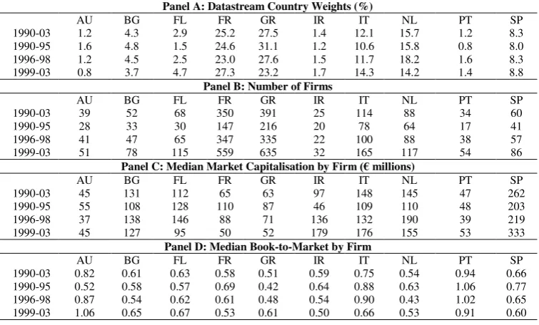
Panel A of Table 1 reveals a stable market share among countries during

1990-2003. France and Germany are the biggest markets with more than a half of the EMU

market capitalisation, regardless of the period. Italy, the Netherlands, and Spain are

median size markets. Their market shares vary from 8% to 18%, depending on the

period being considered. Austria, Belgium, Finland, Ireland, and Portugal are the

smallest markets. All of them present less than 5% of weight in the EMU portfolio at

any point in time. Austria, Ireland, and Portugal with less than 2% are particularly

small.

The number of sample firms used to calculate the size and book-to-market

premiums increases from 1990 to 2003 (see Panel B). The average number of firms

increases from 674 in the first period to 1,892 at the end. This movement has German

and French capital markets as its main representatives. The number of firms from the

biggest markets, contrary to the remaining markets, increase their weight in our sample

- 54% in the first period (363/674) and 63% (1,194/1,892) in the last one. It seems that

this can be explained by the reaction to the development of some new markets,

particularly the Neuer Market and the Nouveau Marché, the German and French

regulated platforms, created respectively in 1997 and in 1996, whose target focuses on

young, small, and high growth stocks (e.g., technology, biotechnology, media and

financial services stocks). The remaining countries also created secondary markets with

the same objective, although without the same success. However, in absolute terms, as it

can be seen in Panel B, the number of firms of each market has been increasing since

the mid 1990s. For example, the number of Portuguese firms increased from 17 to 54.

The reduced interest rates, the development of European capital markets, the economic

growth in the second half of 1990s and the bullish trend, created the ideal atmosphere to

(13)

Panel C shows the median market capitalisation by firm during each sub-period.

The large number of new firms in French and German stock markets caused a decrease

in the median size of firms. On the contrary, Spanish firms experienced an increase in

their market capitalisation, as a result of a comparatively lower increase in the number

of firms. Austrian and Portuguese stock markets, more than the others, are characterised

by a large number of small firms.

Book-to-market by firm is exhibited in Panel D. Austrian and Portuguese stocks

present the highest median value for the book-to-market ratio. As a matter of fact, the

median book-to-market ratio of Austrian stocks shows a tendency to increase - from

0.52 to 1.06. There is also a small decrease in market-to-book of French, Irish, Italian,

and Spanish firms. All other countries manifest no tendency in terms of book-to-market.

3. Empirical Results

The analysis debates the results of CAPM versus FFM, using either the portfolios

(High, Low, Small, and Big) or stocks. The absolute value of the intercept or Jensen’s

alpha, meaning the pricing error, and the adjusted R², which represents the explanatory

power of a model, are used to evaluate the robustness of each model. Sample data is

divided into three sub-periods: 1990-1995, 1996-1998, and 1999-2003. The discussion

is carried out based on the following procedures: First, market excess return, size, and

distress risk premiums, which are used in the local FFM application, are presented;

Second, the results obtained for local, international, and EMU CAPM models, using

High, Low, Small, and Big portfolios, ranked by quintiles, are confronted; Third,

previous results are compared to those obtained with the FFM, in order to: assess how

accurate models based on EMU factors are; evaluate how local size and distress

(14)

and finally, to evaluate international factors, comparing international to local FFM.

Finally, this research compares the robustness of different asset pricing models - local

CAPM, local FFM and international FFM. Models based on EMU factors are excluded

since they reveal poor explanatory power. These results are similar to those found by

Griffin (2002) and Moerman (2005), who concluded that global factors explain to a

lesser extent time-series variation in return and generally have higher pricing errors than

local model.

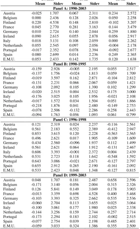
3.1. EMU Local Premiums

Table 2 shows the weekly local market risk premium or domestic market excess return

(DMER), size (DSMB), and distress risk premium (DHML) by country from 1990 to

2003, considering also the following three sub-periods: 1990-95, 1996-98, and

1999-2003.

During 1990-2003 all local market risk premiums followed the same trend.

While market risk premium in the first and the third period were characterised by a

negative return in the majority of European markets, the opposite occurred in the second

period. In the first period, particularly at the beggining, the future Eurozone experienced

a period characterised by high interest rates, as a result of tight monetary policies, and

economic uncertainty about world economic growth and the uncertain result of the

Maastricht Treaty. The last period denotes a correction, after the high-tech bubble in all

stock markets around the world. In contrast, the period from 1996 to 1998 is

(15)

economic perspectives and the investor overreaction, explain the stock market

behaviour.

Analysing the DMER by country, with exception to Finland with 12.08% of

annual risk premium in the whole sample period, the remaining countries present weak

results. Some of the smallest stock markets present the poorest performance. Austria,

Belgium, and Portugal, present an annual DMER of -1.31%, 0.01%, and -0.90%

respectively. However, their performance has been different throughout time. Although

Austria presents, comparatively with the two other countries, a weaker performance in

the first two sub-periods, the poorest results for the two other small markets were in the

first and the third sub-period. Concerning the biggest and median stock markets, the

equity risk premium varies from 0.52% (Germany) to 4.22% (Spain), on an annual

basis. These figures are abnormally low, when compared to the traditional results for

equity risk premium, however, the facts previously reffered to, offer a valuable

explanation for this.3

Size premium (DSMB) reveals, in line with DMER, a uniform behaviour across

European countries. In fact, it is possible to observe signs regarding the existence of that

type of premium whatever the sub-period might be. There are only two countries in the

first and in the second period where the size premium is negative (Belgium and Spain in

the first and Germany and Portugal in the second period). Thus, there are some signs of

size premium on the majority of European markets. Size premium is particulalrly high

in Finland, France and Germany. For example, in the French case, the difference

between Small and Big portfolios excess return is 15.73%, on an annual basis, for all

the sample.

(16)

Concerning book-to-market premium (DHML), our results are less

homogeneous than those obtained by Fama and French (1998). They find a

book-to-market premium in 11 of 12 stock book-to-markets of its own sample, while we only find the

book-to-market premium in 6 - Austria, Belgium, France, Germany, Ireland, and Spain -

of 10 stock markets analysed. However, we can also observe a similar performance

around the sample. For all the sample, there are only two stock markets where the

distress premium is notoriously negative (Finland and Portugal). These results must be

attributed to the second sub-period. From 1996 to 1998 the book-to-market premium is

negative for the majority of countries - Austria, Belgium, France, Germany, Ireland, and

Spain. However, in the remaining sub-periods, particularly in the last one, signs of

financial distress premium are more homogeneous. In fact, with the exception of

Portugal, all stock markets present a financial distress premium in such period.

Previous findings are a result of institutional and economic changes that

European capital markets witness after the single currency. In fact, the single currency

and consequently the lower interest rates, as well as the high-tech euphoria during the

second half of 1990s, could explain the stock price behaviour of growth firms.

Probably, asset managers did not use the more advisable figures for the cost of equity of

growth firms. They estimated a lower cost of equity for growth stocks, substantially

increasing their market prices; that is, asset managers used a lower estimate for

cost-of-equity, creating the ideal conditions for stock prices to overreact. That should explain

what happened after 1999, a sustainable correction of stock market throughout this

(17)

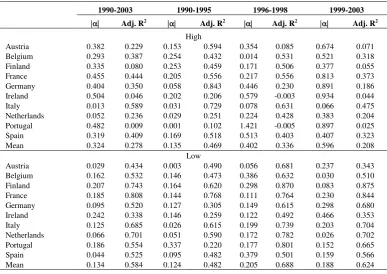
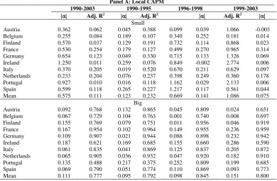
3.2. Local, International, and EMU CAPM: Country Analysis

Table 3, Panels A-C, show the results of regressions for excess return of High and Low

portfolios. Top and bottom quintiles are used as the dependent variable. Local CAPM,

represented by a local factor, international CAPM, defined by a local and international

factor, and EMU CAPM, by an EMU factor, are the three specifications considered in

Table 3. Table 4 presents an identical analysis, although it considers the excess return of

Small and Big portfolios, as the dependent variable.

Analysing the whole period, the primary result regards to the lower performance

of the EMU CAPM. Indeed, we observe in both Table 3 and 4 a higher absolute

Jensen’s alpha and lower adjusted R² in comparison with Local and International

CAPM. For example, for Low portfolios (see Table 3, Panels A, B, and C) the Jensen’s

alpha is, on average, 0.134%, 0.132%, and 0.153%, respectively for local, international,

and EMU CAPM, and the adjusted R² is 58.4%, 59.4%, and 40.4%. For Big portfolios

(see Table 4, Panels A, B, and C), the Jensen’s alpha is, on average 0.111%, 0.111%,

and 0.130%, and the adjusted R² is 77.7%, 78.0%, and 48.7%. These results are, in

general, similar in the sub-periods. Comparing either EMU CAPM to local FFM or

EMU CAPM with international FFM it is possible to show that the former is less

accurate than local and international CAPM. On average, considering 120 portfolios (10

countries; 3 periods; 4 categories of portfolios), the following Jensen’s alpha were

obtained: 0.344% for EMU model, 0.322% for international model, and 0.323% for

local model (see Table 7, Panel A). The difference between Jensen’s alpha of EMU

model and international model (0.022% (1.15% on an annual basis)) presented in Panel

(18)

Jensen’s alpha of EMU model and local model also shows that the difference between

both means (0.021%) is also statistically insignificant (p-value = 0.69).

Panels A-C of Tables 3 and 4 show the absolute intercept for a variety of models

and portfolios. The tendency reaches a steep decrease in the realm of pricing accuracy

during the sample. In fact, there are signs that the intercept increased since the

beginning of 1990s. For example, Jensen’s alpha for High portfolios, considering the

local CAPM, increased from 0.135% in the first period, to 0.596% after 1999 (see Table

3, Panel A); for Big portfolios, the intercept of local CAPM increased from 0.095% to

0.151% (see Table 4, Panel A). The specific risk, measured by the absolute intercept,

has had a more decisive role in matter of pricing in comparison with systematic risk.

The singularity, the small size and the financial structure of new firms can be plausible

explanations for such result. Results are more evident for High and Small portfolios (see

Tabels 3 and 4). For example, considering the international CAPM, whilst the intercept

of Low portfolios changes, on average, from 0.126% to 0.186%, the High portfolio

changes from 0.114% to 0.601% (see Table 3, Panel B). The results for adjusted R² are

in line with Jensen’s alpha. Inversely, for example, the average adjusted R² for High

portfolios, taking into consideration the international CAPM, decreases from 47.5% to

21.9%, the Low portfolios increases from 48.4% to 62.6% (see Panel B, Table 3).

Comparing the local and the international CAPM (see Tables 3 and 4) a slight

difference is observed in the explanatory power between both models. The adjusted R²

of the International CAPM is higher, on average, than that obtained for local CAPM

(0.45%).4 The use of foreign factor produces an increase in adjusted R², which varies,

on average, from 0.1% (80.1%-80.0%), in the case of Big portfolio in the third period,

(19)

to 1.5% (24.7%-23.2%), in the case of Small portfolio and in the first period.

Additionally, a country comparison does not show supremacy of international CAPM.

For example, Panel A, shows adjusted R² of Austrian High portfolio being reduced in

the first period, after foreign factor had been introduced - 59.4% in comparison to

59.3% (see Table 3, Panels A and B).

3.3. Local, International and EMU FFM: Country Analysis

Panels A-C of Tables 5 and 6 show the regressions of High, Low, Small and Big

portfolios excess returns using local, international and EMU FFM.

The first result that must be highlighted for the EMU FFM, as for the EMU

CAPM, concerns its poor results. In fact, the mean alpha of Jensen for 120 portfolios

(10 countries; 3 periods; 4 categories of portfolios) is 0.276%, 0.208%, and 0.225%

respectively for EMU FFM, international FFM, and local FFM (see Panel A, Table 7).

According to Panel B, Table 7 the difference between the mean alpha of Jensen using

EMU and international FFM (0.068%) is statistically significant (p-value = 0.07).

However, the same can not be witnessed when comparing the mean difference of

Jensen’s alphas of EMU FFM and local FFM (0.051%, but p-value = 0.19), as well as

when the results of international and local FFM are confronted (0.018% and p-value =

0.57). Although results not always present statistical significance there are signs that

regressions of local and international FFM present higher explanatory power (higher

adjusted R²) and accuracy (lower absolute intercept) than those obtained using EMU

(20)

intercept (adjusted R²) of 0.212% (48.4%), 0.190% (50.0%), and 0.239% (25.8%),

respectively for local, international, and EMU FFM (see Table 5).

As for the CAPM, the debate seems to be concerned to the local and

international FFM. Therefore, the question is whether the introduction of foreign factors

produces better portfolio excess return estimates. If Jensen’s alpha of international FFM

experienced a recent decrease, then we should conclude that there are some signs of

market integration in EMU stock markets. In order to evaluate the impact of different

factors, (i) local FFM results are compared to those obtained for local CAPM, as a

means of assessing local factors (DSMB and SHML), and (ii) international FFM

compares with local FFM, showing how valuable international factors (FMER, FSMB,

and FSMB) are.

The results of local FFM and local CAPM show that there exist some benefits in

employing the first model. In fact, if all country portfolios and sub-periods exhibited in

Tables 3-6, Panels A and B are considered - 120 portfolios (10 countries; 4 portfolios; 3

periods) –the mean Jensen’s alpha for the local CAPM is higher than that obtained for

the local FFM (0.323% and 0.225% respectively). In fact, the difference between both

means (0.097%) is statistically significant (p-value = 0.03), that is, the introduction of

local factors increases model’s accuracy (see panel B, Table 7). This result can also be

extended to explanatory power. The mean adjusted R2 of the local CAPM and FFM for

different portfolios and periods is 47.44% and 61.21% respectively. Thus, the

introduction of size and financial distress premiums seem to be important to produce

more accurate results, or in other words, as a means of reducing the asset pricing errors.

However, the benefit of using both premiums is not similar for all portfolios. While for

(21)

errors, the opposite occurs when analyses refer to H and S. Hence, the difference on

mean’s asset pricing error of portfolios H, L, S, and B – estimates are based on periods

and countries, that is 30 observations by category of portfolio – of using local FFM

instead of local FFM is -0.163% (p-value = 0.02), -0.014% (p-value = 0.62), -0.250%

(p-value = 0.07), and 0.038% (p-value = 0.12) respectively (see Panel B, Table 7). Thus,

there are signs to indicate that local FFM is more useful when someone is evaluating a

portfolio of small and high book-to-market firms.

Concerning local and international FFM, the results show that there is a slight

increase in terms of explanatory power and accuracy. The average adjusted R² of the

120 portfolios is 62.17% and 61.21%, respectively for international and local FFM. The

adjusted R² difference between the international and local FFM is 0.96%

(62.17%-61.21%), on average, as a result of the inclusion of the three international factors, while

the difference between the local FFM and local CAPM is 13.77% (61.21%-47.44%).

However, the difference between the mean Jensen’s alpha of both models (-0.018%) is

statistically insignificant (p-value = 0.57). Contrarily to the comparison between local

FFM and local CAPM there is no difference between the mean Jensen’s alpha for

different categories of portfolios. The difference on mean of Jensen’s alpha for

portfolios H, L, S, and B is -0.035%, -0.008%, -0.021%, and -0.006% respectively (see

Panel D, Table 7).

Summing up, whilst the role of International FFM seems to be less relevant than

would be expected, local FFM produces better expected portfolio excess returns

estimates than local CAPM.

Although the impact of foreign factors in portfolio excess return is reduced, it is

(22)

each stock market. For that purpose we use the difference between the mean Jensen’s

alpha of international and local FFM as dependent variable, and the average market

capitalisation share of each market relative to each sub-period, as the independent

variable.

Figure 1 shows that the difference between mean of Jensen’s alpha of

international and local FFM increases with the stock market capitalisation share,

regardless of the period being considered. That is, the larger the stock market is the

higher difference on mean Jensen’s alpha of international and local FFM is. The market

share coefficient is statistical significant at the 10% level (t-statistic = -1.73). However,

the impact of size is higher in the last sub-period (see Figure 2). That is, the use of

international FFM produces lower asset pricing errors in last sub-period for large capital

markets. In fact, the market share coefficient, on one hand, is statistically significant in

the last sub-period (t-statistic = -2.09), and on the other hand, size has more impact on

changing in asset pricing errors (-0.157 in all period compared to -0.488). Thus, there

are some signs of financial integration in large capital markets from EMU, in

comparison to small capital markets, particularly after the introduction of single

currency. In fact, results from using foreign factors in large capital markets outperform

the smallest ones.

3.4. Individual Stock Analysis: Local CAPM and Local and International FFM

Table 8 displays the results for individual stock excess returns using the local CAPM,

local FFM, and international FFM. The main objective of comparing local CAPM and

(23)

comparison between local and international FFM claims to evaluate the level of

integration in firms with different characteristics. For a firm to be included in the

sample it is necessary to have significant data, at least, during one sub-period. Hence,

there are data for 486 stocks during the sample period and 533, 846, and 1,408 for each

sub-period.

Table 8 demonstrates how size and book-to-market premium are valuable in

order to explain excess stock return, comparing local FFM to local CAPM. Regressions

for the 1990-2003 period show a 3.2% (16.3%-13.1%) increase on adjusted R², on

average, and a 0.006% (0.142%-0.148%) decreases in the absolute intercept.5

Comparing the local and international FFM results we can observe a slight increase in

explanatory power (1% = 17.3%-16.3%), and a similar absolute intercept (0.142%).

Thus, either for portfolio, or for stocks, particularly to the former, the introduction of

local premiums improves the modelling accuracy and explanatory power, contrarily to

foreign premiums, whose value is ambiguous.

In the first sub-period, local FFM regressions present an explanatory power on

average 5.1% (24.3%-19.2%) higher than local CAPM regressions, as well as a lower

absolute intercept (-0.001% = 0.171%-0.172%). In the second sub-period, the adjusted

R² increases 3.8% (19.6%-15.8%) and an intercept decrease of 0.031%

(0.296%-0.327%) if local factors were included. Finally from 1999 to 2003, explanatory power

changes 3.1% (11.4%-8.3%) increase in explanatory power and accuracy 0.028%

(0.288%-0.316%).

The inclusion of international factors, on average, and in comparison with local

FFM, produces a reduced impact on the regression explanatory power, 0.7%

5

(24)

24.3%), 1% (20.6%-19.6%) and 1.1% (12.5%-11.4%), respectively in the first, second

and the third sub-periods. In regard to intercept, the introduction of international factors

produces the average following variation, 0.009% (0.180%-0.171%), 0.030%

(0.326%-0.296%) and 0.016% (0.304%-0.288%). Thus, the use of international FFM to estimate

stock excess return seems inappropriate since asset pricing errors increase with the

inclusion of foreign factors. The inclusion of new firms in our sample, some of them

with non-synchronous trading, explains why intercept increases, on average, throughout

the sample.

4. Out-of-Sample Analysis: Firm and Portfolio Analysis

In this section, the results obtained through local CAPM and local and international

FFM are used to evaluate if there are differences when portfolio and firm expected

returns are being forecasted.

EMU FFM is not considered in this section because prior results, in the line of

those obtained by Griffin (2002) and Moerman (2005), show that EMU FFM

underperform all specifications in terms of pricing error and explanatory power.

1.4.1. Expected Cost of Capital

Table 9 presents estimates for the cost of equity by firm. Annual estimates for a firm’s

cost of equity are obtained using weekly average returns from 1990 to 2003. Following

assumptions are applied: (1) only firms whose systematic risk is statistically significant

(25)

local annual risk premium is on the interval {E[RPannual]  1.5 annualRP}; (3) intercept

terms are excluded because estimates of cost of equity are more accurate under such

circumstance (see Fama and French (1997)). Thus, on average, the sample considers

estimates for cost of equity in 578 firms. France and Ireland are the countries most and

least represented in the sample with 156 and 11 firms respectively.

Table 9 shows that the expected stock excess return in some small stock markets

underperforms those obtained for large stock markets, namely in Austria, Belgium and

Portugal. The results vary from 4.55% to 6.55%, on average. In the opposite extreme of

our sample are Finland, Ireland, and Netherlands whose estimates are always higher

than 9.25%, whatever the specification used. Contrarily to expected, the cost-of capital

is smaller for firms of small countries because the sample of those countries include

comparatively a large percentage of big firms.

The difference obtained for local CAPM and FFM estimates are relatively

comparable with Fama and French (1997). In their research, comparing local CAPM

and FFM, they find a 2% difference in the cost of equity for seventeen industries. In our

research, estimates for both models are different in 1.03% (9.30%-8.27%), in average.

Although there are countries where such difference is higher than 2.5%, on average,

such as is the case in Finland and Netherlands, there are also countries where there is no

difference in the estimates for cost of equity, namely for Italy. However, those results

must be analysed with caution, because they are dependent of the sample of firms. For

example, if a large firm is selected, a lower cost of equity using FFM is expected since

it will have a size discount.

The comparison between estimates for cost of equity, using local and

(26)

((10.07%-9.30%)/9.30%). However, the results are not similar around the sample.

While in Germany a 0.22% difference ((9.20%-9.22%)/9.22%) between estimates for

both models is identified, in Italy a 27.87% difference is observed.

Summing up, our results are in line with the conclusion of Griffin (2002), who

concludes that the choice of a local or international FFM has a significant impact on the

cost of equity estimates.

1.4.2. Out-of-Sample Analysis: Firm and Portfolio Analysis

In this section the sample of firms and assumptions presented in 1.4.1 is used. Its main

objective is to forecast errors of stock and portfolio excess returns. That is, the

difference between weekly average return and the weekly expected return of a stock (or

a portfolio), during a year. Errors are forecasted based on weekly mean estimates of a

year, during 1991 to 2004. Expected average return of a stock or a portfolio, during a

year, is calculated based on estimates obtained for different specifications (local CAPM,

local FFM, and international FFM) in the year before forecasting a error. For example,

to forecast an error of stock excess return in 1991 it is necessary to estimate different

specifications during 1990.

Panel A of Table 10 presents forecasted errors of stock excess returns. For that

purpose the following expression is used:



 

 T

t n

i

it it E r

r N

T 1 1

) ( 1

1

(27)

where r_i_tis the weekly average return of a stock i in year t and E(r_it) is the expected

stock return for the same period, using the previous models, as well as prior

assumptions. N is the number of stocks.

On the other hand, in Panel B are presented forecasted errors of portfolio excess

return, in value weighted-basis, considering the stocks used in Panel A:



 



T

i n

i

it it

it T

t n

i it

r E r MV

MV 1 1

1 1

) ( (

1

(1.5)

where MVi is the average market capitalisation of a firm i in year t.

Analysing the forecasted errors, size and distress risk premium seem to be more

advisable factors to evaluate portfolio than stock excess returns. In fact, the introduction

of those two factors produces more accurate estimates for portfolios, because while the

use of local FFM in comparison with local CAPM produces, on average, a decrease of

8.82% for stocks - ((0.74%-0.68%)/0.68%) - in terms of accuracy, for portfolios we

observe an increase of 5.66% - ((0.50%-0.53%)/0.53%).

On the other hand, comparing local and the international FFM there is a small

difference in terms of forecasting power, although international FFM presents poorer

results. In fact, the introduction of the three new factors increases the amplitude of

forecasted errors. Forecasted errors change, on average, from 0.74% to 0.77% and from

0.50% to 0.51%, respectively in case of excess stock returns and excess portfolio

(28)

1.5. Conclusion

The main objective of this research is to evaluate whether the biggest stock markets of

EMU are becoming centralised and the smallest peripheral. For that purpose, different

alternative CAPM and FFM specifications are compared, which consider different local

and foreign factors.

In line with Griffin (2002) and Moerman (2005), this research shows that models

based on global factors are less accurate than models based on local and foreign factors.

There are also important signs to illustrate that international factors produce

more accurate estimates in larger capital markets, particularly after the introduction of

single currency. Thus, it seems that the largest firms are becoming integrated between

themselves, and the smallest are becoming segmented.

This paper also shows that the choice of model’s specification has a significant

impact on the cost-of-equity estimates, as Fama and French (1997) and Griffin (2002)

conclude.

Finally, results reveal that the use of domestic size and book-to-market risk seem

to be more advisable factors to consider for portfolio than for firm. International factors,

on the other hand, seem to be inadequate to estimate either portfolio or stock excess

(29)

References

Adjaouté, K., and J. Danthine, 2003, European financial integration and equity returns: A theory-based assessment, Working Paper, International Center for Financial Asset Management and Engineering.

Bhandari, L., 1988, Debt/Equity Ratio and Expected Common Stock Returns: Empirical Evidence, Journal of Finance, 1988, 43, 507-528

Banz, R., 1981, The relation between return and market value of common stocks, Journal of Financial Economics 9, 3-18.

Basu, S., 1977, Investment performance of common stocks in relation to their price-earnings: A test of the efficient market hypothesis, Journal of Finance 32, 663-682.

Bekaert, G., and C. Harvey, 1995, Time-varying world market integration, Journal of Finance 32, 663-682.

Berk, J., 1995, A critique of size-related anomalies, Review of Financial Studies 8, 275-286.

Brunner, R., K. Eades, R. Harris, and R. Higgins, 1998, Best practices in estimating the cost of capital: Survey and synthesis, Financial Practice and Education 8, 13-28.

Carvalho, C., 2004, Cross-border securities clearing and settlement infrastructure in the European Union as a prerequisite to financial markets integration: Challenges and perspectives, Working Paper, Hamburg Institute of International Economics.

Chan, L., Y. Hamao, and J. Lakonishok, 1991, Fundamentals and stock returns in Japan, Journal of Finance 46, 1739-1764.

Dahlquist, M., L. Pinkowitz, R. Stulz, and R. Wlliamson, 2003, Corporate governance and the home bias, Journal of Financial and Quantitative Analysis 38, 87-110.

Damodaran, A., 1992, Investment valuation (John Wiley).

Errunza, V., and D. Miller, 2000, Market segmentation and the cost of capital in international equity markets, Journal of Financial and Quantitative Analysis 35, 577-600.

Errunza, V., and E. Losq, 1985, International asset pricing under mild segmentation: Theory and test, Journal of Finance 40, 105-124.

Fama, E., and K. French, 1993, Common risk factors in the returns on stocks and bonds, Journal of Financial Economics 33, 3-56.

(30)

Fama, E., and K. French, 1998, Value versus growth: The international evidence, Journal of Finance 53, 1975-1999.

Fratzscher. M., 2001, Financial market integration in Europe: On the effects of EMU on stock markets, Working Paper, European Central Bank.

Graham, J., and C. Harvey, 2001, The theory and practice of corporate finance: Evidence from the field, Journal of Financial Economics 60, 187-243.

Griffin, J., 2002, Are the Fama and French factors global or country specific?, Review of Financial Studies 15, 187-243.

Grinblatt, M., and M. Keloharju, 2001, How distance, language, and culture influence stock-holdings and trades, Journal of Finance 56, 1053-1073.

Hardouvelis, G., D. Malliaropulos, and R. Priestley, 2001, EMU and European stock market integration, http://ssrn.com/abstract=280775.

Hardouvelis, G., D. Malliaropulos, and R. Priestley, 2004, The impact of globalization on the equity cost of capital, Working Paper, Center for Economic and Policy Research.

Harvey, C., 1991, The world price of covariance risk, Journal of Finance 46, 111-157.

Harvey, C., 1995, Predictable risk and returns in emerging markets, Review of Financial Studies 8, 773-816.

Jorion, P., and E. Schwartz, 1986, Integration vs segmentation in the Canadian stock market, Journal of Finance 41, 603-614.

Kang, J., and R. Stulz, 1997, Why there is a home bias? An analysis of foreign portfolio equity ownership in Japan, Journal of Financial Economics 46, 3-28.

Karolyi, G., 1998, Why do companies list shares abroad?: A survey of the evidence and its managerial implications, Financial Markets, Institutions & Instruments 7, Number 1.

Lakonishok, J., A. Shleifer, and R. Vishny, 1994, Contrarian investment, extrapolation, and Risk, Journal of Finance 49, 1541-1578.

Lintner, J., 1965, The valuation of risk assets and the selection of risky investments in stock portfolios and capital budgets, Review of Economics and Statistics 47, 13-37.

Moerman, G., 2005, How domestic is the Fama and French three-factor model? An application to the Euro area, Working Paper, Erasmus Research Institute of Management.

Newey, W., and K. West, 1987, A simple, positive semi-definite, heteroskedasticity and autocorrelation consistent covariance matrix, Econometrica 55, 703-708.

(31)

Sharpe, W., 1964, Capital asset prices: A theory of capital market equilibrium under conditions of risk, Journal of Finance 19, 425-442.

Solnik, B., 1974, The international pricing of risk: An empirical investigation of the world capital market structure, Journal of Finance 29, 365-378.

Stehle, R., 1977, An empirical test of the alternative hypothesis of national and international pricing of risky assets, Journal of Finance 32, 365-378.

(32)

[image:32.595.122.500.143.371.2]

Table 1: Sample Description by Countries

AU, BG, FL, FR, GR, IR, IT, NL, PT, and SP are respectively Austria, Belgium, Finland, France, Germany, Ireland, Italy, the Netherlands, Portugal, and Spain. Panel A shows Datastream country weights in the EMU portfolio. Panel B indicates annual average number of firms by period used to build the size and the distress risk premiums. Panel C indicates the median size of firms in Panel B. Panels D indicates the median book-to-market of firms in Panel B.

Panel A: Datastream Country Weights (%)

AU BG FL FR GR IR IT NL PT SP

1990-03 1.2 4.3 2.9 25.2 27.5 1.4 12.1 15.7 1.2 8.3 1990-95 1.6 4.8 1.5 24.6 31.1 1.2 10.6 15.8 0.8 8.0 1996-98 1.2 4.5 2.5 23.0 27.6 1.5 11.7 18.2 1.6 8.3 1999-03 0.8 3.7 4.7 27.3 23.2 1.7 14.3 14.2 1.4 8.8

Panel B: Number of Firms

1990-03 39 52 68 350 391 25 114 88 34 60

1990-95 28 33 30 147 216 20 78 64 17 41

1996-98 41 47 65 347 335 22 100 88 38 57 1999-03 51 78 115 559 635 32 165 117 54 86

Panel C: Median Market Capitalisation by Firm (€ millions)

1990-03 45 131 112 65 63 97 148 145 47 262 1990-95 55 108 128 110 87 46 109 110 48 203 1996-98 37 138 146 88 71 136 132 190 39 219 1999-03 45 127 95 50 52 179 176 155 53 333

Panel D: Median Book-to-Market by Firm

(33)

[image:33.595.165.446.154.613.2]

Table 2: Descriptive Statistics of Variables

Domestic market excess return (DMER) is obtained, considering a DS country indices and Germany Euro-mark one month, as proxies for market return and risk-free-asset. Small minus big (DSMB) is the return difference between S (small firms) and B (big firms) domestic portfolios. High minus low (DHML) is the return difference between H (high book-to-market firms) and L (low book-to-market firms) domestic portfolios. EMU results are value-weighted. Variables are weekly means, calculated on a value-weighted basis, for the following four periods: 1990-1995; 1996-1998; 1999-2003; and 1990-2003. Results are a weekly percentage.

DMER SMB HML

Mean Stdev Mean Stdev Mean Stdev Panel A: 1990-2003

Austria -0.025 1.707 0.067 2.311 0.234 2.572 Belgium 0.000 2.436 0.128 2.026 0.050 2.258 Finland 0.220 4.538 0.148 2.810 -0.102 3.207 France 0.045 2.770 0.281 3.163 0.144 3.479 Germany 0.010 2.724 0.140 2.044 0.259 1.880 Ireland 0.090 2.615 0.055 2.878 0.056 2.917 Italy 0.018 3.131 0.108 2.059 0.000 2.262 Netherlands 0.055 2.545 0.097 2.056 -0.004 2.178 Portugal -0.017 2.352 0.078 2.394 -0.092 2.677 Spain 0.080 2.699 0.014 2.236 0.249 2.365 E.M.U. 0.053 2.433 0.142 1.735 0.120 1.638

Panel B: 1990-1995

Austria -0.159 2.926 -0.005 2.195 0.055 2.517 Belgium -0.137 1.756 -0.024 1.813 0.059 1.709 Finland -0.019 3.597 0.162 2.871 -0.104 2.812 France -0.131 2.231 0.066 2.067 0.059 1.421 Germany -0.108 2.092 0.105 1.390 0.102 1.299 Ireland -0.020 2.515 0.004 2.532 0.175 3.000 Italy -0.176 3.025 0.105 1.956 -0.021 2.108 Netherlands -0.017 1.572 0.034 1.504 0.051 1.866 Portugal -0.218 1.876 0.041 2.480 -0.149 2.753 Spain -0.078 2.506 -0.132 2.286 0.258 2.443 E.M.U. -0.094 1.763 0.056 1.093 0.061 0.799

Panel C: 1996-1998

Austria 0.121 2.319 0.024 2.237 -0.116 2.561 Belgium 0.561 2.183 0.552 2.389 -0.412 2.947 Finland 0.853 3.615 0.120 2.228 -0.563 2.565 France 0.496 2.621 0.017 1.905 -0.109 1.609 Germany 0.434 2.560 -0.096 1.937 0.112 1.499 Ireland 0.561 2.621 0.064 1.912 -0.131 2.467 Italy 0.606 3.393 -0.001 2.372 0.004 2.439 Netherlands 0.531 2.723 0.118 1.642 -0.548 1.592 Portugal 0.643 3.086 -0.021 2.671 -0.127 2.797 Spain 0.655 2.912 0.265 2.190 -0.161 2.092 E.M.U. 0.533 2.423 0.048 1.348 -0.127 0.815

Panel D: 1999-2003

(34)

[image:34.595.130.518.217.491.2]

Table 3: Excess Returns of High and Low Portfolios using CAPM

High and Low portfolios excess returns are dependent variables. They represent the top and bottom quintile. Variables are value-weighted, calculated on a weekly basis for the following periods: 1990-1995; 1996-1998; 1999-2003, and 1990-2003. DS country indices are used as local market proxy. Germany Euro-Mark one-month is the risk-free asset proxy. The method of estimation is ordinary least squares, using the Newey and West (1987) covariance estimator that is consistent in the presence of both heteroskedasticity and autocorrelation of unknown form. Domestic Model is a result of regression ri,t= i + b Di(wDt-1DMERt) + εi,t,

where ri,t is the portfolio (High or Low) excess return in period t, DMER is the domestic excess return, and 

is a constant. wDt-1is the weight of a local portfolio in EMU. b Diis the unconditional sensitivity of asset i to

the factor. EMU Model is a result of regression: ri,t = i+ bi(EMERt) + εi,t, where EMERt represents the EMU

factor. It is also calculated using a value-weighted basis. EMERt= wDt-1DMERt+ wFt-1FMERt, where wDt-1 and

wFt-1are respectively the weight of local and foreign portfolios in the EMU portfolio in the week t-1.

International Model is the result of regression: ri,t= i+ b Di(wDt-1 DMERt) + b Fi (wFt-1FMERt) + εi,t.

Panel A: Local CAPM

1990-2003 1990-1995 1996-1998 1999-2003  Adj. R2 _ _{Adj. R}2 _ _{Adj. R}2 _ _{Adj. R}2

High

Austria 0.382 0.229 0.153 0.594 0.354 0.085 0.674 0.071 Belgium 0.293 0.387 0.254 0.432 0.014 0.531 0.521 0.318 Finland 0.335 0.080 0.253 0.459 0.171 0.506 0.377 0.055 France 0.455 0.444 0.205 0.556 0.217 0.556 0.813 0.373 Germany 0.404 0.350 0.058 0.843 0.446 0.230 0.891 0.186 Ireland 0.504 0.046 0.202 0.206 0.579 -0.003 0.934 0.044 Italy 0.013 0.589 0.031 0.729 0.078 0.631 0.066 0.475 Netherlands 0.052 0.236 0.029 0.251 0.224 0.428 0.383 0.204 Portugal 0.482 0.009 0.001 0.102 1.421 -0.005 0.897 0.025 Spain 0.319 0.409 0.169 0.518 0.513 0.403 0.407 0.323 Mean 0.324 0.278 0.135 0.469 0.402 0.336 0.596 0.208

Low

(35)

Panel B: International CAPM

1990-2003 1990-1995 1996-1998 1999-2003  Adj. R2  Adj. R2  Adj. R2  Adj. R2

High

Low

Austria 0.034 0.436 0.000 0.489 0.061 0.679 0.247 0.347 Belgium 0.163 0.532 0.145 0.474 0.382 0.632 0.022 0.513 Finland 0.215 0.750 0.158 0.619 0.321 0.876 0.057 0.877 France 0.185 0.808 0.145 0.769 0.141 0.770 0.226 0.844 Germany 0.073 0.548 0.125 0.309 0.110 0.621 0.297 0.679 Ireland 0.245 0.382 0.157 0.260 0.103 0.495 0.469 0.354 Italy 0.120 0.688 0.030 0.618 0.163 0.744 0.206 0.703 Netherlands 0.067 0.701 0.067 0.601 0.164 0.782 0.033 0.702 Portugal 0.182 0.564 0.341 0.224 0.148 0.803 0.144 0.672 Spain 0.040 0.530 0.095 0.481 0.375 0.499 0.158 0.572 Mean 0.132 0.594 0.126 0.484 0.197 0.690 0.186 0.626

Panel C: EMU CAPM High

Low

(36)

[image:36.595.140.531.207.462.2]

Table 4: Excess Returns of Small and Big Portfolios using CAPM

Small and Big portfolios excess returns are dependent variables. They represent the top and bottom quintile. Variables are value-weighted, calculated on a weekly basis for the following periods: 1990-1995; 1996-1998; 1999-2003, and 1990-2003. DS country indices are used as local market proxy. Germany Euro-Mark one-month is the risk-free asset proxy. The method of estimation is ordinary least squares, using the Newey and West (1987) covariance estimator that is consistent in the presence of both heteroskedasticity and autocorrelation of unknown form. Domestic Model is a result of regression ri,t = i+ b Di(wDt-1DMERt) + εi,t, where ri,t is the portfolio (High or Low) excess

return in period t, DMER is the domestic excess return, and  is a constant. wDt-1is the weight of a local portfolio in

EMU. b Diis the unconditional sensitivity of asset i to the factor. EMU Model is a result of regression: ri,t = i+ bi

(EMERt) + εi,t, where EMERt represents the EMU factor. It is also calculated using a value-weighted basis. EMERt=

wDt-1DMERt+ wFt-1FMERt, where wDt-1and wFt-1are respectively the weight of local and foreign portfolios in the

EMU portfolio in the week t-1. International Model is the result of regression: ri,t = i + b Di(wDt-1DMERt) + b Fi(wFt-1

FMERt) + εi,t.

Panel A: Local CAPM

1990-2003 1990-1995 1996-1998 1999-2003  Adj. R2 _ _{Adj. R}2 _ _{Adj. R}2 _

Small

Austria 0.362 0.062 0.045 0.388 0.099 0.039 1.066 -0.003 Belgium 0.255 0.084 0.189 0.107 0.349 0.252 0.181 0.014 Finland 0.570 0.037 0.129 0.191 0.732 0.114 0.868 0.023 France 0.530 0.254 0.179 0.127 0.499 0.270 0.965 0.314 Germany 0.654 0.123 0.049 0.330 0.715 0.133 1.326 0.069 Ireland 1.250 0.011 0.259 0.076 0.849 -0.002 2.774 0.006 Italy 0.370 0.205 0.019 0.520 0.670 0.211 0.629 0.097 Netherlands 0.233 0.204 0.076 0.237 0.398 0.249 0.360 0.178 Portugal 0.927 0.010 0.016 0.118 1.162 0.029 2.133 0.006 Spain 0.599 0.118 0.265 0.227 1.217 0.117 0.561 0.044 Mean 0.575 0.111 0.123 0.232 0.669 0.141 1.086 0.075

Big

(37)

Panel B: International CAPM

1990-2003 1990-1995 1996-1998 1999-2003  Adj. R2 _ _{Adj. R}2 _a _{Adj. R}2 _a _{Adj. R}2

Small

Austria 0.363 0.061 0.042 0.387 0.108 0.033 1.073 -0.007 Belgium 0.252 0.085 0.187 0.112 0.347 0.248 0.178 0.011 Finland 0.581 0.062 0.143 0.191 0.696 0.139 0.919 0.037 France 0.522 0.271 0.187 0.193 0.472 0.284 0.974 0.315 Germany 0.653 0.122 0.052 0.350 0.693 0.130 1.328 0.068 Ireland 1.252 0.011 0.269 0.074 0.905 0.002 2.776 0.007 Italy 0.368 0.204 0.027 0.530 0.669 0.206 0.624 0.095 Netherlands 0.240 0.218 0.081 0.236 0.385 0.249 0.319 0.211 Portugal 0.919 0.013 0.031 0.160 1.139 0.024 2.117 0.004 Spain 0.603 0.119 0.292 0.236 1.175 0.129 0.561 0.041 Mean 0.575 0.116 0.131 0.247 0.659 0.144 1.087 0.078

Big

Panel C: EMU CAPM Small

Austria 0.335 0.010 0.072 0.173 0.067 0.015 1.081 -0.003 Belgium 0.243 0.064 0.170 0.092 0.407 0.193 0.170 0.011 Finland 0.596 0.060 0.218 0.051 0.726 0.138 0.933 0.040 France 0.520 0.269 0.188 0.194 0.468 0.283 0.986 0.311 Germany 0.642 0.106 0.049 0.333 0.673 0.127 1.321 0.055 Ireland 1.270 0.009 0.308 0.030 0.959 -0.006 2.768 0.010 Italy 0.353 0.146 0.002 0.325 0.665 0.136 0.605 0.090 Netherlands 0.249 0.210 0.111 0.163 0.391 0.232 0.326 0.213 Portugal 0.930 0.011 0.045 0.106 1.171 0.016 2.028 0.003 Spain 0.631 0.095 0.321 0.184 1.229 0.127 0.558 0.036 Mean 0.577 0.098 0.148 0.165 0.676 0.126 1.078 0.077

Big

(38)

[image:38.595.132.504.279.545.2]

Table 5: Excess Returns of High and Low Portfolios using FFM

High and Low portfolios excess returns are dependent variables. They represent the top and bottom quintile. Variables are value-weighted, calculated on a weekly basis for the following periods: 1990-1995; 1996-1998; 1999-2003, and 1990-2003. DS country indices are used as local market proxy. Germany Euro-Mark one-month is the risk-free asset proxy. The method of estimation is ordinary least squares, using the Newey and West (1987) covariance estimator that is consistent in the presence of both heteroskedasticity and autocorrelation of unknown form. Domestic Model is a result of regression ri,t = i+ b Di(wDt-1DMERt) + sD i(wDt-1DSMBt) + h Di(wD t-1DHMLt) + εi,t, where ri,t is the portfolio (High or Low) excess return in period t, DMER is the domestic excess

return, DSMB is the return difference between S (local small firms) and B (logal big firms), DHML is the return difference between H (high book-to-market firms) and L (low book-to-market firms), and  is a constant. wDt-1is

the weight of a local portfolio in EMU. b Di, sDi,, and h Di are the unconditional sensitivities of asset i to the factors. EMU Model is a result of regression: ri,t = i+ bi(EMERt) + si(ESMBt) + hi(EHMLt) + εi,t, where

EMERt ESMB, and EHML represent EMU factors. They are calculated considering the countries weight in the EMU portfolio. Thus, we have, for example, EMERt= wDt-1DMERt+ wFt-1FMERt, where wDt-1and wFt-1are

respectively the weight of local and foreign portfolios in the EMU portfolio in the week t-1. International Model is the result of regression: ri,t = i+ b Di(wDt-1DMERt) + sD i(wDt-1DSMBt) + h Di(wDt-1DHMLt) + b Fi(wFt-1

FMERt) + sF i(wFt-1FSMBt) + h Fi(wFt-1FHMLt) + εi,t.

Panel A: Local FFM

1990-2003 1990-1995 1996-1998 1999-2003  Adj. R2 _ _{Adj. R}2 _ _{Adj. R}2 _ _{Adj. R}2

High

Low