Tariff Policy, Increasing Returns and Endogenous Fluctuations

Munich Personal RePEc Archive

Tariff Policy, Increasing Returns and

Endogenous Fluctuations

Chen, Yan and Zhang, Yan

Shandong University, Shanghai Jiaotong University and New York

University

17 August 2008

Online at

https://mpra.ub.uni-muenchen.de/10061/

Tari¤ Policy, Increasing Returns and Endogenous

Fluctuations

Chen Yany

Shandong University

Zhang Yanz

Shanghai Jiao-Tong University

August 17, 2008

Preliminary draft, please don’t quote without the authors’ permission. We wish to thank Wen Yi for helpful comments and Kevin Lansing for his criticisms on the old version of this paper. We especially thank Prof. Jess Benhabib for encouraging us to write this paper. All the remaining errors are ours.

y_{Center for Economic Research, Shandong University, 27 Shanda Nanlu, Jinan, Shandong, China,}

250100. Tel: 86-531-88369046. E-mail: [email protected].

z_{Assistant Professor, Economics Department, School of Economics, Antai College of Economics &}

Running Title: Tari¤ Policy and Endogenous Fluctuations

Abstract: We study the e¤ects of government tari¤ policy in a one-sector small open economy RBC model with a productive externality that generates social increasing returns to scale. Various forms of endogenous ‡uctuations, including stable 2-, 4-, 8-, and 15-cycles, quasiperiodic orbits and chaos can be identi…ed in this model if we introduce a constant tari¤ or subsidy (applied to the imported production factor) into the laissez-faire economy that exhibits local indeterminacy. In a somewhat di¤erent model, Guo and Lansing (2002) show that a constant capital tax or subsidy can give rise to similar dynamics in a closed-economy one sector model with a productive externality. From this perspective, factor income taxes and tari¤s are equivalent to generate endogenous ‡uctuations in those economies with social increasing returns to scale. We further show that in our model, the local determinacy can coexist with the global indeterminacy for a plausible range of tari¤ rates, which brings our attention to the use of local steady state analysis to make conclusions about the global dynamics of the nonlinear models.

Key Words: Tari¤ Policy, Global Indeterminacy, Chaos.

1. Introduction

It is well understood by now that those economies with incomplete markets, imperfect competition or externalities can be easily pushed into the instability, exhibiting

endoge-nous cycles, indeterminacy or chaos1. The government usually uses monetary and …scal

policies to address those issues related to the aggregate instability. We show that in a standard one sector small open economy Ramsey model with a productive externality, if the government wants to use the tari¤ policy to close the gap between the social and private marginal products of imported energy (which is created by the productive ex-ternality), it can give rise to various forms of endogenous dynamics, such as bifurcations and chaos.

Our framework is a discrete-time version of the one-sector small open economy growth model, recently developed by Wen and Aguiar-Conraria (2005, 2006 and 2007 henceforth WAC) [based on Benhabib and Farmer (1994)]. WAC show that in the small open economy with the imported energy as a third production factor, as long as the positive production externality is strong enough, the model can exhibit “local indeterminacy” around the single interior steady state.

We start our project by solving for a benchmark tari¤ policy that closes the gap be-tween the social and private marginal products of imported energy in the WAC struc-ture. The benchmark policy involves constant subsidy (negative tari¤) rates applied to imported energy incomes. We show that the tari¤ rate applied to imported energy incomes is a key bifurcation parameter for the model’s dynamics. In a laissez-faire econ-omy that exhibits local indeterminacy, the dynamical system will undergo a supercritical Hopf bifurcation as the tari¤ rate becomes su¢ciently negative (representing a subsidy) and a supercritical ‡ip bifurcation as the tari¤ rate becomes su¢ciently positive. An attracting closed orbit or cycle emerges as the tari¤ rate passes those critical values.

Pushing the tari¤ rate beyond the critical value ( f lip _{) in either direction may give}

way to chaos.

For the numerical calibration, the ‡ip bifurcation occurs at the tari¤ rate of 26.33 percent. As the tari¤ rate is further increased beyond the ‡ip bifurcation value, the model exhibits a series of period-doubling bifurcations–a typical route to chaos. This

means that stable 2-, 4-, and 8- cycles, even chaos may appear as varies. The economic

region of parameter space, the substitution e¤ect generated by expected movements in the after-tax interest rate overcomes the corresponding income e¤ect by an amount that is su¢cient to induce cycling in agents’ optimal saving decisions...".

For tari¤ rates beyond the ‡ip-bifurcation value, the equilibrium is saddle-path sta-ble. However, the local determinacy of equilibrium near the steady state coexists with global indeterminacy, which means that in regions away from the steady state, a stable n-period cycle or a chaotic attractor can arise as the equilibrium paths.

The Hopf bifurcation occurs at the energy subsidy rate of 51.14 percent. If the gov-ernment wants to encourage energy imports by setting the subsidy at or more than 51.14 percent, it will destabilize the steady state and allow for Hopf bifurcations and regular 15-cycles. As the subsidy rate is increased beyond the Hopf-bifurcation value of 51.14 percent, an attracting closed orbit will surround the steady state and quasi-periodic oscillations arise. Further increases in the subsidy rate may make the orbit break up into a regular 15-cycle. The economic explanation can also be found in the paper of Guo and Lansing (2002, page 635), "...The high-subsidy region is characterized by large intermittent spikes in hours worked which re‡ect a “bunching e¤ect” in production as agents’ decisions internalize more of the increasing returns...".

Before solving the model and doing the quantitative simulations, we brie‡y mention some other papers that are closely related to the contributions of ours. Some of those papers are Cazzavillan (1996), Guo and Lansing (2002) and Coury and Wen (2008). All of the above papers are concerned with indeterminacy issues near a single interior steady state. In the spirit, our paper is very close to Guo and Lansing (2002)’s work because both analyze the …scal policy under the framework with social increasing returns to scale.

The remainder of the paper is organized as follows. Section 2 introduces tari¤ policy into the WAC model. Section 3 studies the model’s dynamics with constant subsidy/tari¤ rates. Section 4 discusses some extensions. Section 5 concludes.

2. The Basic Model

externality for the ease of interpretation.

2.1. Households

The in…nitely-lived representative household, endowed with one unit of time, maximizes a discounted stream of utilities over her lifetime by choosing sequences of consumption

fctg1t=0, hours to work fntg1t=0, and the stock of capitalfkt+1g1t=0:

max

1

X

t=0

t_(logc t B

n1+_t

1 + ),B >0, (1)

where 2(0;1)is the discount factor and 0denotes the inverse of the intertemporal

elasticity of substitution in labor supply. We assume that no intrinsic uncertainties are present in the economy.

The household’s budget constraint is

ct+it=rtkt+wtnt+Tt, (2)

where it is investment, kt is the household’s stock of physical capital, rt is the capital

rental rate, wt denotes the real wage and Tt is the lump-sum transfer/tax, i.e., Tt can

be negative. The household receives income by supplying capital and labor services

to …rms. Fiscal policy parameters in our model include: (1) the variable Tt, which

represents the lump-sum tari¤ transfer to the agent; and (2) the implicit …scal policy

parameter – the tari¤ or subsidy rate imposed on the imported energy (say oil). Under this framework, negative tari¤ rates represent energy subsidies and a negative value of

Tt represents a lump-sum tax received by the government. The household views rt,wt

and Tt as being exogenously given.

Investment follows the law of motion of capital,

kt+1= (1 )kt+it,k0 given, (3)

The …rst-order conditions for the household’s optimization problem are given by

Bn_t = wt

ct

, (4)

1

ct

=

ct+1

(rt+1+ 1 ), (5)

and the transversality condition is

lim

t!1 tkt+1

ct

= 0. (6)

Equation (4) requires that the household’s marginal rate of substitution between consumption and leisure be equal. Equation (5) is the consumption Euler equation.

2.2. Firms

The representative …rm produces a homogenous …nal good using the following constant returns to scale technology:

yt=ztktakn an t o

ao

t , (7)

whereytis the …rm’s output,otis the third factor, say imported oil andak+an+ao = 1,

i.e., constant returns to scale at the …rm level. zt is the state of technology or the

production externality that the …rm takes as given. Each …rm chooses fkt; nt; otg to

maximize pro…ts by solving

= max

kt;nt;otyt rtkt wtnt p o_{(1 +}

t)ot, (8)

subject to equation (7), where t is the tari¤ rate imposed on the imported oil. We

assume that factor markets are perfectly competitive. The pro…t maximization implies

rt = ak yt kt

, (9)

wt = an yt nt

, (10)

po(1 + t) = ao yt ot

From equation (11), we have po_o

t=aoyt=(1 + t).

In contrast to a standard RBC model, the state of technology or the production

externalityzt, is given by

zt= (KtakN an t O

ao

t ) , 0, (12)

where Kt, Ht and Ot are the economy-wide average input levels. In the (symmetric)

equilibrium, all …rms act in the same way such that Kt = kt, Ht = ht and Ot = ot.

Hence, the social technology is given by

yt=ktkntnoto, (13)

where k ak(1 + ), n an(1 + ) and o ao(1 + ). The social technology

exhibits increasing returns to scale ( k+ n+ o >1) for >0.2

Assuming that the foreign input is perfectly elastically supplied, then the factor

price, po_{, is independent of the factor demand for o. Thus, we have o}

t = _po₍₁₊aoyt t).

Substituting this formula into the production function, we can obtain the following reduced-form production function:

yt=Ak k 1 o t n

n 1 o

t , (14)

whereA= ao

po_{(1 +} t)

o 1 o

acts as the technology coe¢cient in a neoclassical growth

model, which is inversely related to the foreign factor price. In the reduced-form

pro-duction function, the e¤ective returns to scale is measured by k+ n

1 o , which exceeds the

real returns to scale,

k+ n

1 o

>( k+ n+ o)

2.3. Government

We assume that there is no government spending and the government transfers the tari¤ revenue to the households. The government balances the budget in each period:

Tt= tpoot= ao t

Using equations (2), (3), (9), (10) and po_o

t = aoyt=(1 + ), we obtain the following

aggregate resource constraint equation:

kt+1= (1 )kt+yt 1 ao

1 + t

ct. (15)

3. Dynamics with Constant Tari¤/Subsidy Rates

As in Guo and Lansing (2002), the increasing-returns technology (13) introduces a nonconvexity into the constraint set of the social planner’s problem, which makes the

Kuhn-Tucker su¢ciency theorem not applicable to our …scal policy analysis3. As an

alternative to computing the optimal tari¤ policy, we consider the following benchmark tari¤ policy that closes the gap between the social and private marginal products of the imported energy.

Proposition 1. The wedge between the social and private marginal products of the imported energy is eliminated when t= ₁₊1 1 for all t,Tt= ao ytfor all t.

Proof. The social marginal products from equation (13) is @yt_@ot = oyt=ot. The

after-tari¤ private marginal product is (1 + t) 1ao@yt_@ot. With t = ₁₊1 1 < 0, (1 +

t) 1ao@yt_@ot = oyt=ot. The lump-sum tari¤ revenue follows directly from equation

Tt= tpoot= ₁₊ao t_tyt= ao yt.

The benchmark policy involves constant subsidy rates that are only governed by the externality parameter . A similar result is also obtained in Guo and Lansing’s model. In the following analysis, we assume the tari¤ rate is constant, which implies that the government income is endogenous.

3.1. Calibration (Quantitative Experiments)

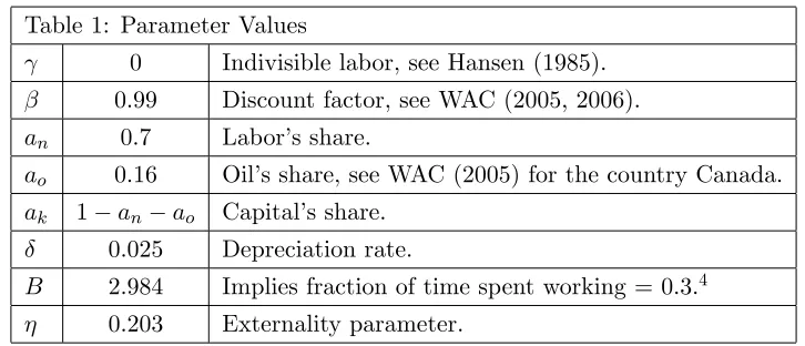
According to the existing RBC literature, we calibrate the structural parameters for a quarterly model. Following WAC (2005, 2006 and 2007), table 1 summarizes the baseline parameter values.

Table 1: Parameter Values

0 Indivisible labor, see Hansen (1985).

0:99 Discount factor, see WAC (2005, 2006).

an 0:7 Labor’s share.

ao 0:16 Oil’s share, see WAC (2005) for the country Canada.

ak 1 an ao Capital’s share.

0:025 Depreciation rate.

B 2:984 Implies fraction of time spent working = 0.3.4

0:203 Externality parameter.

The baseline parameter values are commonly used in real business cycle models

except the externality parameter 5_{. The degree of returns to scale in the model is1+ .}

WAC (2005) note that minimal returns to scale needed to generate local indeterminacy can vary dramatically depending on the degree of energy dependence of that speci…c country.

Given our baseline parameter values, it requires returns to scale at least 1.198 to

exhibit local indeterminacy. We let = 0:203for our quantitative experiments, which

implies returns to scale around 1.203 and the benchmark …scal policy parameter b ₌

1

1+ 1 = 0:16874. This experiment makes the laissez-faire economy exhibit local

3.2. Log-Linearized Dynamics

In the appendix, we show that the equilibrium conditions in our model can be described by the following log-linear system:

"

ln kt+1=k

ln (ct+1=c)

#

=

2

4 _{1 3}1 2

4

1 2 3 4

3

5

| {z }

J

"

ln kt=k

ln (ct=c)

#

,k0 given, (16)

wherekand care steady-state values of capital and consumption andJ_{denotes a2 2}

Jacobian matrix of partial derivatives evaluated at the steady-state solution for the

original dynamic system. The elements of J _{can be represented by four constants, i,}

i= 1,2,3,4, which expressions can be found in the appendix. ( i can be represented

by the model parameters B, ak, an, ao, , , and .) The two eigenvalues of J will

determine the stability of the log-linear system. The oil price po _{does not appear in}

J _{and thus will not a¤ect the model’s local stability properties. Equations (4) and}

(5) show that not only a¤ects the tradeo¤ between consumption and leisure at a

given date (it can be seen from (4)) but also a¤ects the tradeo¤ between consumption goods at di¤erent dates (it can be seen from (5)). As Guo and Lansing (2002, page 641) pointed out, "...the intertemporal tradeo¤ is the crucial mechanism for generating multiple equilibria because agents’ expectations of future returns must become self-ful…lling...".

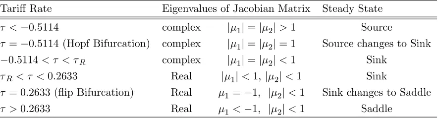
Table 2 summarizes the model’s local stability properties as we allow the tari¤ rate

to vary from 1 to+1.

Tari¤ Rate Eigenvalues of Jacobian Matrix Steady State

< 0:5114 complex j ₁j=j ₂j>1 Source

= 0:5114(Hopf Bifurcation) complex j ₁j=j ₂j= 1 Source changes to Sink

0:5114< < R complex j 1j=j 2j<1 Sink

R< <0:2633 Real j 1j<1,j 2j<1 Sink

= 0:2633(‡ip Bifurcation) Real ₁= 1, j ₂j<1 Sink changes to Saddle

>0:2633 Real ₁< 1, j ₂j<1 Saddle

3.3. Local Indeterminacy

Figure 1 plots the combinations of (the externality parameter) and (the tari¤ rate)

that allow for di¤erent equilibrium dynamics. Local indeterminacy requires that both

eigenvalues of J _{lie inside the unit circle. We know that the degree of returns to scale}

in the model is 1 + . When = 0 (CRS), the model is saddle point stable for all

values of . The …gure shows that >0:1976is needed for the steady state to become

locally indeterminate. Given > 0:1976, decreases in eventually makes the steady

state become a source while increases in eventually make the steady state become

a saddle point. We set to be 0.203 in the calibration and the local indeterminacy

occurs for tari¤ rates in the range 0:5114 < < 0:2633. When > 0:2633, the

model exhibits a locally unique equilibrium (a saddle point). Hence, if the government wants to stabilize the economy against sunspot ‡uctuations near the steady state by imposing a su¢ciently high tari¤ rate on the imports, instead such a policy may make the economy susceptible to other forms of endogenous ‡uctuations, such as bifurcations and/or chaos.

Insert Figure 1 here

3.4. Flip Bifurcation

For the numerical experiment, the dynamical system undergoes a ‡ip bifurcation as

is increased past the value f lip _{= 0:2633. We …rst prove that the ‡ip bifurcation point}

is supercritical. This means that, within a small open neighborhood of f lip (in our

case f lip_{+"), and as increases, the steady state goes from being a sink to being a}

saddle surrounded by an attracting period–2 cycle6. At the bifurcation point, we have

det(J) +tr(J) = 1(see Guo and Lansing (2002)). Using the expressions fordet(J)and

tr(J_{) derived in the appendix, we can get the following bifurcation value}7_:

f lip ₌ aoH1( + )

H1( + ) +ak(H2 H1)

1, (17)

where 1= 1 is the household’s rate of time preference. In this model, we use

numerical simulations to establish that the ‡ip bifurcation is supercritical8_{. The}

converge to the steady state. The two-cycle is an attractor and in this case, the global indeterminacy coexists with local determinacy because the steady state is a saddle point

for >0:2633. If we set >0:2633in oder to eliminate sunspot ‡uctuations near the

steady state, it can make the economy susceptible to sunspots, cycles, or even chaos, in regions away from the steady state.

3.5. Hopf Bifurcation

For the numerical calibration, the dynamic system undergoes a Hopf bifurcation as

is decreased past the value Hopf _{= 0:5114}9_{. At the Hopf bifurcation point, we have}

det(J_{) = 1(see Guo and Lansing (2002)). Using the expression fordet(}J_{)derived in the}

appendix, we get the following bifurcation value10:

Hopf ₌ aoM4( + )

M4( + ) ak[ +M1 ( + )]

1. (18)

We use numerical simulations to establish that the Hopf bifurcation in our model is

supercritical. In the supercritical Hopf bifurcation, an attracting closed orbit emerges

on the side of Hopf where the steady state is unstable (in our case a source), that is,

in the small neighborhood Hopf _".

The supercritical Hopf bifurcation makes our model exhibit deterministic, quasiperi-odic oscillations that won’t converge to the steady state. Because the invariant closed orbit is an attractor, there exists a continuum of equilibrium paths each leading to the closed orbit. This is a case of global indeterminacy.

3.6. Nonlinear Dynamics

The model’s perfect foresight dynamics follow the nonlinear map: (see the appendix)

ct+1

2

6 4akAk

k+ o 1 1 o t+1

0

@anA

B k

k 1 o t+1

ct+1

1

A

n (1+ )(1 o) n

+ 1

3

7 5= _c1

t

, (19)

kt+1 = 1

ao

1 + Ak

k 1 o t

0

@anA

B k k 1 o t ct 1 A n (1+ )(1 o) n

To simulate the global dynamics, we iterate the above map for a range of values of . Following Guo and Lansing (2002), the iteration proceeds as follows. We disturb the

steady state by an arbitrary amount and set our initial values (k0, c0), then we solve

equation (20) fork1. Substituting the value of k1 into equation (19) yields a nonlinear

equation that can be used to solvec1. We can repeat the procedure to compute(k2,c2)

and so on.

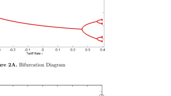
Figure 2 plots the bifurcation diagram and the largest Lyapunov exponent over

the range 0:51172 0:39780. Figure 3 and 4 show the details near Hopf _and

f lip_{. The bifurcation diagram gives us the long-run behavior of the model by plotting}

the last 250 points of a long simulation. The …gures show that setting the tari¤ rate

beyond f lip _{eventually leads to chaos. Since as increases, a signi…cantly positive}

Lyapunov exponent occurs, which is an indicator of "sensitive dependence on initial

conditions"—one of the characteristics of chaos11_{. The transition to chaos takes place}

via a "period-doubling" route in the high-tari¤ rate region ( > f lip_).

Insert Figures 2, 3 and 4 here

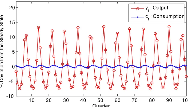
Figures 5 to 9 show us various forms of endogenous ‡uctuations as varies. Figures

5 and 6 show that the Hopf bifurcation is supercritical since the invariant closed orbit is

attracting. As = Hopf 2:1E 4, rational expectations equilibrium paths eventually

converge to the invariant closed orbit for arbitrary starting points either inside or outside the circle. Figure 7 shows that the invariant closed orbit starts to break up into a regular

15-cycle when the tari¤ rate is decreased to some point in the left hand side of Hopf_.

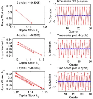
In the small neighborhood of the ‡ip bifurcation point, the model exhibits stable 2- and

4- and 8-cycles for tari¤ rates in the range of f lip _{< < 0:39780. Figure 8 depicts}

these three kinds of cycles and their corresponding time-series simulated data. When we

increase the value of the tari¤ rate to = 0:39775, a type of chaotic attractors emerges

as shown in …gure 9.

Changes in have e¤ect on the amplitude of the cycles or oscillations. In the high–

the stable n-cycle as a kind of rational expectations equilibria can be explained in the similar way like Guo and Lansing (2002, page 652)"...the substitution e¤ect generated by expected movements in the after-tari¤ interest rate overcomes the corresponding income e¤ect by an amount that is su¢cient to induce cycling in agents’ optimal saving decisions...".

The time series plots in …gures 5 through 9 give us a picture about the percentage changes in model output and consumption. These …gures indicate that the consump-tion is quite smooth, while the output is quite volatile. The ‡uctuaconsump-tion amplitudes of output is much larger than those observed in the real Canada economy at business-cycle frequencies. It can be due to the presence of strong increasing returns.

Insert Figures 5, 6, 7, 8 and 9 here

4. Extension: Local Control—Adjustment Costs

In this section, similar to Guo and Lansing (2002), we describe some policy mechanisms which are used to eliminate sunspot ‡uctuations near the steady state.

It is well known that explicit adjustment costs for capital investment can be used to select a locally unique equilibrium. We then consider an economy where the household budget constraint (2) is described by the following new equation:

ct+it

2

6 6 6

41 + 2

kt+1

kt

1

2

| {z }

t( )

3

7 7 7

5=rtkt+wtnt; (21)

the adjustment cost parameter can be used as the bifurcation parameter. Given other

parameter values in our baseline model, the dynamical system undergoes a supercritical

‡ip bifurcation as is increased past the value0:1781.

5. Conclusion

In this paper, we introduce a constant tari¤ or subsidy rate (applied to the imported energy) into the WAC (2005, 2006 and 2007) model. In this setting, our dynamical equilibrium is described by a two-dimensional di¤erence equations system with one preditermined variable (capital). And we …nd that a rich set of endogenous ‡uctuations including bifurcations and/or chaos can arise in this setup. The dynamical system undergoes a supercritical Hopf bifurcation as the tari¤ rate becomes su¢ciently negative, and a supercritical ‡ip bifurcation as the tari¤ rate becomes su¢ciently positive. The model’s equilibrium dynamics exhibit stable 2-, 4-, 8-, and 15-cycles, quasi-periodic closed orbits, and chaos. In a somewhat di¤erent model, Guo and Lansing (2002) show that a constant capital tax or subsidy can give rise to similar dynamics in a closed-economy one sector model with a productive externality. From this perspective, factor income taxes and tari¤s are equivalent to generate endogenous ‡uctuations.

Notes:

1. See Benhabib and Farmer (1999) for an excellent survey of the literature.

2. We only consider the case k <1, which says that the externality is not strong

enough to generate sustained endogenous growth.

3. As Guo and Lansing (2002) pointed out, the nonconvexity will make it hard for us to compute the …rst-best allocations and …nd the optimal …scal policy which implements the …rst-best as a competitive equilibrium.

4. Since our calibration exercise is a numerical experiment, we simply set the implied faction of time spent on working to be 0.3, which is used in Guo and Lansing (2002). Though 0.3 may not be exactly the one of Canada, we say our results will be robust for reasonable parameter selection. Usually, people work 8 hours per day.

5. We should mention that our results are robust to the parameterpo_{. In our case,}

we setpo _{= 0:1.}

6. See Guckenheimer and Holmes (1983).

7. ForH1 and H2, see our appendix.

8. For the analytical calculation, see Guckenheimer and Holmes (1983). 9. For the analytical calculation, see Guckenheimer and Holmes (1983).

10. ForM1 and M4, see our appendix.

ex-ponents according to the procedure described by Alligood et. al. (1997). Since

equa-tion (19) cannot be solved explicitly for ct+1, the required derivatives @ct+1=@kt and

@ct+1=@ct are computed numerically by log-linearizing equation (19) around each

suc-cessive point of the trajectory generated by the nonlinear map. This introduces some approximation error into our computation so that values of the Lyapunov exponent that are only slightly above zero are not reliable indicators of chaos."

References

[1] Alligood, K.T., T.D. Sauer, and J.A. Yorke (1997). Chaos: An Introduction to Dynamical Systems. New York: Springer-Verlag.

[2] Benhabib, J. and R.E. Farmer (1994). Indeterminacy and increasing returns. Jour-nal of Economic Theory 63, 19–41.

[3] Benhabib, J. and R.E. Farmer (1999). Indeterminacy and sunspots in macroeco-nomics. In: Taylor, J.B., Woodford, M. (Eds.), Handbook of Macroeconomics, vol. 1A. North-Holland, New York, pp. 387–448.

[4] Cazzavillan, G. (1996). Public Spending, Endogenous Growth, and Endogenous Fluctuations, Journal of Economic Theory, 71, 394-415.

[5] Coury, T. and Y. Wen (2008), Global Indeterminacy in Locally Determinate RBC Models, FORTHCOMING: International Journal of Economic Theory.

[6] Guckenheimer, J. and P. Holmes. (1983). Nonlinear Oscillations, Dynamical Sys-tems, and Bifurcations of Vector Fields. New York: Springer-Verlag.

[7] Guo, J.T. and K.J. Lansing (2002). Fiscal policy, increasing returns and endogeous ‡uctuations. Macroeconomic Dynamics 6, 633-664.

[8] Hansen, G.D. (1985). Indivisible Labor and the Business Cycle, Journal of Mone-tary Economics, 16, 309-327.

[10] Wen, Y. and L. Aguiai-Conraria. (2006). Oil dependence and economic instability, Federal Reserve bank of St. Louis, 2006.

Appendix:

This part gives us the equations used to study the model’s equilibrium dynamics in section 3.

The equilibrium conditions can be seen from the following four equations:

yt = Ak k 1 o t n

n 1 o

t , whereA=

ao po_{(1 + )}

o 1 o

, (E-1)

Bn1+_t = an yt ct , (E-2) 1 ct =

ct+1

ak yt+1

kt+1

+ 1 , (E-3)

ct+kt+1 = (1 )kt+yt 1 ao

1 + . (E-4)

For the parameter values in Table 1, we can see that there is a unique interior steady state in this economy. Equations (E.1) and (E.2) imply:

nt =

0

@anA

B k k 1 o t ct 1 A 1 o (1+ )(1 o) n

= anA

B

1 o (1+ )(1 o) n

k

k (1+ )(1 o) n

t c

1 o (1+ )(1 o) n

t .

which can be used to substitute nt in equations (E.3) and (E.4). Thus, we can imply

equations (19) and (20).

In the small neighborhood of the steady state, equations (19) and (20) can be ap-proximated by the log-linearization method and we have:

"

ln kt+1=k

ln (ct+1=c)

#

=

2

4 _{1 3}1 2

4

1 2 3 4

3

5

| {z }

J

"

ln kt=k

ln (ct=c)

#

,k0 given,

where the four main elements are: 1 = M4+1 +M4

c

M3 = (1+ )(_{(1+ )(1}k+ o_o)1)+_nn and M4 = _{(1+ )(1}k(1+ )_{o) n}. The steady state capital/labor

ratio c

k =

+

ak 1 ao

1+ . 1= 1is the household’s rate of time preference.

The determinant and trace of J are:

det(J) = 1

4

, (E-5)

trace(J) = 1+

1 2 3 4

. (E-6)

At the Hopf bifurcation point, we havedet(J) = 1, and at the ‡ip bifurcation point,

we havedet(J) +trace(J) = 1.

At the Hopf bifurcation point,det(J) = 1, say,

M4 +

ak

1 ao

1 + = M4 M1 ( + ),

Hopf ₌ aoM4( + )

M4( + ) ak[ +M1 ( + )]

1.

At the ‡ip bifurcation point,det(J) +trace(J) = 1, say,

2 M1 ( + )

= M4+ 1 +M4

c

k [2 +M1 ( + )]

h

M1+ (1 +M1)

c k

i

M3 ( + ).

RHS = c

kf2M4+ ( + ) [M1(M4 M3) M3]g+ 2 M4+ 2 (1 )

+ ( + ) [M1M4 +M1 M1 M1M3 ];

c

kf2M4+ ( + ) [M1(M4 M3) M3]g

= 4 2 + 2 M4+ ( + ) [M1M4 + 2M1 M1 M1M3 ]

= 4 2 + 2 M4+ ( + ) [ M1(M4 M3) + (2 )M1];

DenoteH1,H2 as

H1 = 2M4+ ( + ) [M1(M4 M3) M3]

and H2 = 4 2 + 2 M4+ ( + ) [ M1(M4 M3) + (2 )M1], then we have

H1

+

ak

1 ao

1 + =H2,

f lip =

aoH1( + )

H1( + ) +ak(H2 H1)

6. Figures

-1 -0.9 -0.8 -0.7 -0.6-0.5 -0.4 -0.3 -0.2 -0.1 0 0.1 0.2 0.3 0.4 0.5 0.6 0.7 0.8 0.9 1 0.19

0.192 0.194 0.196 0.198 0.2 0.202 0.204

Saddle Source

Source

Sink

Det = 1

Det + Tr = -1

Saddle

Figure 2A. Bifurcation Diagram

-0.5 -0.4 -0.3 -0.2 -0.1 0 0.1 0.2 0.3 0.4 -2

-1.75 -1.5 -1.25 -1 -0.75 -0.5 -0.25 0 0.25 0.5

Tariff Rateτ

L

ar

ge

s

t

L

y

na

pu

n

ov

E

x

po

n

en

t

LE>0

-0.512 -0.5115 -0.511 -0.5105 0.32

0.34 0.36 0.38 0.4 0.42 0.44 0.46

Tariff Rateτ

Ho

ur

s

W

or

k

ed

h t

Figure 3A. Bifurcation Diagram (Details Near Hopf_).

-0.512 -0.5115 -0.511 -0.5105

-0.1 -0.05 0 0.05 0.1

Tariff Rate τ

La

rgest

Ly

a

pun

ov

E

x

po

nen

t

Figure 4A. Bifurcation Diagram (Detail Near f lip₎

0.2 0.25 0.3 0.35 0.4

-0.25 -0.2 -0.15 -0.1 -0.05 0 0.05 0.1 0.15

Tariff Rateτ

Lar

ge

s

t

Ly

apunov

E

x

pon

ent

LE > 0

2.3 2.32 2.34 2.36 2.38 2.4 2.42 0.34

0.36 0.38 0.4 0.42 0.44 0.46

Capital Stock k

t

H

ou

rs

Wor

ke

d

h t

Figure 5A. Phase Diagram (Attacting Circle—Start Inside): = Hopf _{2:1E 4}

10 20 30 40 50 60 70 80 90 100

-10 -5 0 5 10 15 20

Quarter

%

De

v

ia

ti

on

from

th

e

S

te

a

dy S

ta

te

y

t : Output c

t : Cons um ption

2.28 2.3 2.32 2.34 2.36 2.38 2.4 2.42 0.34

0.36 0.38 0.4 0.42 0.44 0.46

Capital Stock k t

Ho

ur

s

W

or

k

ed

h t

Figure 6A. Phase Diagram (Attacting Circle—Start Outside): = Hopf _{2:1E 4}

10 20 30 40 50 60 70 80 90 100

-10 -5 0 5 10 15 20

Quarter

%

Dev

iat

ion

fr

o

m

t

h

e

S

teady

S

tat

e

y

t : Output

c_t : Cons umption

2.3 2.32 2.34 2.36 2.38 2.4 2.42 0.35

0.4

Capital Stock k t

Hours

W

o

rk

ed

h

t

Figure 7A. Long–Run Phase Diagram (Attracting 15-Cycle): = Hopf _{3:7E 4}

10 20 30 40 50 60 70 80 90 100

-10 -5 0 5 10 15 20

Quarter

% D

ev

iati

on fr

om

the S

teady

S

tate

y t : Output c

t : Cons um ption

1.16 1.18 1.2 0.26 0.28 0.3 0.32 H ours Work e d h t

Capital Stock k

t

2-cycle (τ=0.3008)

1.12 1.14 1.16

0.24 0.26 0.28 0.3 0.32 0.34

Capital Stock k

t H ours Work e d h t

4-cycle (τ=0.3858)

1.12 1.14 1.16

0.24 0.26 0.28 0.3 0.32

Capital Stock k

t H ours Work e d h t

8-cycle (τ=0.3953)

10 20 30

-5 0 5 10 Quarter % D ev iat ion

Time-series plot (2-cycle)

10 20 30

-10 0 10 Quarter % D ev iat ion

Time-series plot (4-cycle)

10 20 30 40

-10 0 10

Time-series plot (8-cycle)

Quarter % D ev iat ion c b a

1.115 1.12 1.125 1.13 1.135 1.14 1.145 1.15 1.155 1.16 0.24

0.25 0.26 0.27 0.28 0.29 0.3 0.31 0.32 0.33

Capital Stock k

t

H

ours

Work

ed

h t

Figure 9A. Phase Diagram (Chaotic Attractor): = 0:39775:

0 10 20 30 40 50 60 70 80 90 100 110 120 130 140 150

-15 -10 -5 0 5 10 15 20 25

Quarter

%

D

ev

iat

io

n

y

t : Output

c

t : Consumption