Abstract—This work examines the identification of a
mathematical model of the thermal performance of a building, based on experimental data available for direct measurement. The authors offer a new model structure with a reduced number of parameters. An identification method based on building an inverse dynamics model that uses exponential filtration is considered. The method makes it possible to estimate signals that cannot be measured directly: the signal of the general perturbation of the indoor air temperature and the signal of specific heat loss through the building envelope. A simulated example is given of identifying the thermal performance of a building based on test data using VisSim visual modeling software.
The identification method offered in the article may be used in engineering calculations for designing automatic control systems and in predictive control algorithms for heating buildings.
Index Terms—Building thermal conditions model,
exponential filtration, heating of buildings, identification.
I. INTRODUCTION
NE of the main objectives in the development of urban engineering infrastructure in countries with moderate climates is to improve the energy efficiency of building heating systems [1], [2]. The modern approach to saving thermal energy when heating buildings and increasing the comfort of building users assumes the introduction of automatic control systems that use model predictive control methods [3]–[6]. Another important issue is the development and identification of a mathematical model for building heating parameters [7]–[10].
The indoor air temperature Тind of a building depends on its volume, building envelope type, the quantity of applied thermal energy Qsource, inner and external perturbing factors such as the outdoor air temperature Тout, solar radiation Jrad, wind Vwind, internal heat release Qint, and the building’s accumulated internal thermal energy Qacc (Fig. 1).
However, the signals Тind, Qsource, and Тout presented in Fig. 1 can be measured quite easily in practice, while direct
Manuscript received March 17, 2013; revised April 3, 2013.
V. V. Abdullin is with the Automatics and Control Department, South Ural State University, Chelyabinsk, Russia (corresponding author to provide phone: +7-351-777-5667; fax: +7-351-267-9135; e-mail: [email protected]).
D. A. Shnayder is with the Automatics and Control Department, South Ural State University, Chelyabinsk, Russia (phone: +7-922-751-1212; e-mail: [email protected]).
L. S. Kazarinov is with the Automatics and Control Department, South Ural State University, Chelyabinsk, Russia (phone: +7-351-267-9011; e-mail: [email protected]).
measurement of Jrad, Vwind, Qint, and Qacc, which affect the temperature Тind, is actually problematic.
Furthermore, it should be noted that the processes of heat transfer are distributed and generally described by partial differential equations [11]. However these equations are not convenient for use in the identification process in their given form, because they contain a large number of parameters which are very difficult to determine in practice. The following is a method to identify the thermal characteristics of a building, based on a reduced set of experimental data, which makes it suitable for practical use.
II. A METHOD TO IDENTIFY
THE THERMAL CHARACTERISTICS OF A BUILDING The initial (empirical) data for modeling the thermal performance of a building include the heating power applied to the building, the outdoor air temperature, and the indoor air temperature. The indoor air temperature Тind of a building, which is the average value of indoor temperatures in each room, accounting for differences in area, is calculated as follows:
ind
ind ,
i i
i
i i
S T t T t
S
(1)where Si, Tind i stand for the area and temperature of the i-th
room, respectively, t is time. Using the average temperature
Tind permits us to estimate relatively fast perturbations – such as wind, solar radiation, or local heat sources, which affect the thermal performance of some rooms, for example, the rooms of one side of the building – for the entire building. We can then assume that the response time of the model’s output signal (indoor air temperature) to these perturbations is comparable to the time constants of the relatively slow processes of heat accumulation and heat loss through a building envelope with high heat capacity.
Consequently, the concept of a general temperature perturbation, Tz, may be introduced, characterizing the
Method of Building Thermal Performance
Identification Based on Exponential Filtration
Vildan V. Abdullin, Dmitry A. Shnayder, Lev S. Kazarinov
O
Building Tout
Jrad Vwind
Qsource Tind
Qind
[image:1.595.318.510.693.775.2]Qacc
effect of the factors mentioned above on the indoor air temperature. Therefore, the heat balance equation takes the following form:
0
ind ind z
0
,
Q t
T t T t T t q V
(2)
where Tind*(t) stands for the predicted value of the indoor air temperature (the prediction horizon is determined by the fluctuation of the indoor air temperature as a result of the perturbing factors (Fig. 1)); Tout(t) is the outdoor air temperature; Q0(t) stands for the heating power applied to the heating system; q0 represents the specific heat loss (per cubic meter); and V is the external volume of the building.
Let us assume that the behavior of the indoor air temperature Tind(t) is described by a linear dynamic operator with a pure delay given by:
d
0( ) ,
j
j p
i i
b p
L p e
a p
(3)where τd is the pure delay time.
A block diagram of a building thermal performance dynamics model composed in accordance with equations (2) and (3) is presented in Fig. 2.
In the model presented in Fig.1, we will consider the values Q0(t), Tout(t), Tind(t) to be known, because they can be directly measured in practice. The unknown values are:
– polynomial coefficients ai and bj (3);
– delay time constant τd; – building specific heat loss q0;
– general temperature perturbation Tz(t);
– predicted value of the indoor air temperature Tind*(t). The values of ai, bj, and τd can be determined from the building’s response to a stepwise change in the heating power Q0(t) using well-known methods, for example,
Matlab’s Ident toolbox (MathWorks, Inc., USA). However, to reduce the effect of the perturbing factors Tout(t) and Tz(t) a series of experiments is conducted, and ai, bj, and τd are calculated according to the following equations:
d d , ,
1 1 1
1 1 1
, , ,
N N N
k i i k j j k
k k k
a a b b
N N N
(4)where N is the number of experiments; k stands for a sequence number of an experiment; and ai,k , bj,k , and τd k
represent the values obtained during the experiment. Next, let us assume that Tind*(t) and Tind(t) are statistically unbiased signals and that Tz(t) is a signal with a mean of zero, then:
ind
ind
,t t
M T t M T t (5)
z
0 ,t
M T t (6)
where Mt{•} is the time-mean operator.
From Equations (2), (5), and (6), it follows that the specific heat loss through the building envelope can be calculated using:
0
0
out ind
.
t
t t
M Q t q
V M T t M T t
(7)
It is evident from (2) that the general perturbation Tz can be determined by:
0
z out ind
0
,
Q t
T t T t T t q V
(8)
where Tind*(t) is the predicted indoor air temperature. According to the model presented in Fig. 1, the predicted indoor air temperature can be determined by the following equation:
1
ind 0 ind ,
T t L T t (9) where L0–1{•} stands for the inverse dynamics operator.
From (3), the operator’s formal inverse is:
1 0
0 0
( ) з .
n m
p
i j
i j
i j
L p a p b p e
(10)
A block diagram of the operator’s formal inverse is presented in Fig. 3.
Let us consider constructing the dynamics operator L0–1{•} based on the exponential filtration method [12].
Let a signal decomposition in polynomial basis be given as follows:
ind
0
( ) ( ) ,
n
i i i
T t g t
(11)where λ is the retrospective interval, and gi(t) stands for the
decomposition’s spectral components.
Considering a prediction at time τd , (11) becomes:
ind d d
0
( ( )) ( )( ) .
n
i i
i
T t g t
(12)epτd
0
1 m
j j j
b p
h(t)
Differential component with a prediction
Tind(t) Tind
*
(t)
φ(t)
n
i i ip
a
[image:2.595.300.547.591.678.2]0
Fig. 3. Block diagram of the operator’s formal inverse.
V q0
1
0 L
о
Q t
outT t
z T t
0 [image:2.595.282.548.707.774.2]T t Tind
t Tind
tAccording to the Newton binomial, we then obtain
d d
0
( ) ( 1) ,
i
i k i k i k
k k
c
(13)where сk stands for the binomial coefficients. Substituting
(13) in (12), we get the relationship for a signal:
ind d d
0 0
( ( )) ( ) ( 1) ,
n i
k i k i k
i k
i k
T t g t c
(14)which accounts for the prediction at time τd.
Then we decompose the signal φ(t) in the polynomial basis: 0 ( ) ( ) . n i i i
t g t
(15)Let us consider the decomposition of the signal φ(t) into the Taylor series:
( )
0
( )
( ) ( 1) .
! i n i i i t t i
(16)Comparing the expressions (15) and (16) yields the following equation:
( )
( ) ( 1) ! ( ) .
i i
i
t i g t
(17)
Equation (17) shows the relationship between the i-th derivative of the input signal φ(i)(t) and the corresponding spectral component gi(t).
Hence, the output of the filter’s differential part, without accounting for the predictive component τd, will become:
( )
0 0
( ) ( ) ( 1) ! ( ) .
n n
i i
i i i
i i
h t a t i a g t
(18)Comparing the expressions (15) and (18), we conclude that obtaining an expression for the signal h(t) requires the following substitution in (14):
( 1) ! .
i i
i
i a
(19)
By applying (19) to (14), we determine the output of the differential component of the predictive filter:
d
0 0
d
0 0
( ) ( ) ( 1) ( 1) !
( 1) ( ) ! .
n i
i k i k k
i k k
i k
n i
i i k
i k k
i k
h t g t c k a g t k c a
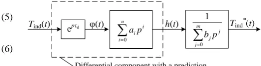
(20)As a result, we obtain the inverse operator structure given in Fig. 4. Here Φinp stands for the exponential filter of input signal moments; Р-1 is the inverse correlation coefficient matrix; А is the coefficient matrix for the differential component of the inverse operator; μ(t) = {μ0(t),
μ1(t), …, μn(t)}T represents the vector of input signals
moments; and g(t) = {g0(t), g1(t), …, gn(t)}Т stands for a
vector of the decomposition’s coordinate functions.
Signal projections {gi(t)} are determined based on the
criterion of minimum exponential mean error in the input signal (11): 2 2 ind 0 1
( ) ( ) i( ) i Т ,
E t T t g t e d T
(21)where Т is the time constant of the averaging filter.
The solution is based on the minimum of function (21) along projections of gi(t):
2( )
0, 0, .
i E t i n g (22)
The solution to problem (22) is a system of recurrence relations [13]
0, 0, 1 ind
, , 1 1,
1 ; 1 1 ; 1 ,
k k k
i k i k i k
k k
t T t T T
i t t T P g μ (23)
where Tind,k stands for the input signal at time tk; Δt is the
time sampling interval, and P = Q–1 represents a matrix of constant coefficient determined from the following relationships:
( )
, ,
|| i j||, i j i j( )!
Q q q T i j (24)
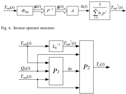
The block diagram of the identification system operating in real-time is presented in Fig. 5. Here P1 is described by (7), and P2 is described by (8).
Q0(t)
Tout(t)
Tind(t)
P
1P
2 1
0 L Tind
* (t)
q0
Tz(t)
Fig. 5. Block diagram of a real-time identification system for signals q0
and Tz(t).
Фinp
Tind(t)
Р -1 А
0 1 m j j j b p
Tind* (t) h(t)
[image:3.595.282.476.321.400.2]g(t) μ(t)
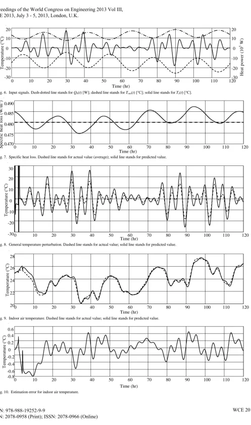
[image:3.595.305.552.577.760.2]Fig. 6. Input signals. Dash-dotted line stands for Q0(t) [W]; dashed line stands for Tout(t) [°С]; solid line stands for Tz(t) [°C].
Fig. 7. Specific heat loss. Dashed line stands for actual value (average); solid line stands for predicted value.
Fig. 8. General temperature perturbation. Dashed line stands for actual value; solid line stands for predicted value.
[image:4.595.54.548.53.174.2]Fig. 9. Indoor air temperature. Dashed line stands for actual value; solid line stands for predicted value.
Fig. 10. Estimation error for indoor air temperature.
Time (hr)
0 10 20 30 40 50 60 70 80 90 100 110 120
T
em
pe
ra
tur
e
(°
C
)
-20 -10 0 10 20
H
ea
t
pow
er
(
10
5 W)
-30 -20 -10 0 10 20
-30
Time (hr)
0 10 20 30 40 50 60 70 80 90 100 110 120
S
pe
ci
fi
c
he
at
l
os
s
(W
/m
3 )
0.470 0.475 0.480 0.485 0.490
Time (hr)
0 10 20 30 40 50 60 70 80 90 100 110 120
T
em
pe
ra
tur
e
(°
C)
-30 -20 -10 0 10 20 30
Time (hr)
0 10 20 30 40 50 60 70 80 90 100 110 120
T
em
pe
ra
tur
e
(°
C
)
20 22 24 26 28
Time (hr)
0 10 20 30 40 50 60 70 80 90 100 110 120
T
em
pe
ra
tur
e
(°
C
)
-0.6 -0.4 -0.2 0 0.2 0.4 0.6
Thus, the proposed method results in real-time identification of the unknown signals q0 and Tz(t) using the measured values of Q0(t), Tout(t) and Tind(t).
III. A SIMULATED EXAMPLE
Let us consider an example of identifying the thermal characteristics of a building based on the proposed method using VisSim visual simulation software (Visual Solutions, Inc., USA).
Let us assume that operator L0(p) is as follows:
d 0
1 2
1
( ) .
(1 ) (1 )
p
L p e
pТ pТ
(25)
Let the parameters for the model presented in Fig. 1 take the following values: V = 7000 m3, q0 = 0.48 W/(m3 °С),
Т1 = 6 hrs, Т2 = 3 hrs, τd = 2 hrs.
Considering the cyclic nature of changes in outdoor air temperature, heat power, and the perturbing factors, let us use the harmonic test signals in Fig. 6 as the model’s input signals Tout(t) and Q0(t) as well as signal Tz(t), which will be defined later in the identification process.
The graph of the corresponding variation in indoor air temperature Tind(t) for the model given in Fig. 2 with dynamics operator (25) is presented in Fig. 9 (solid line).
The dynamics operator (25) is inverted based on the structure of the inverse operator presented in Fig. 4. The target signals q0 and Tz(t) are calculated according to the identification system’s block diagram, presented in Fig. 5.
Fig. 7–10 present the modeling results. Fig. 7 shows graphs of the source- and calculated signals of specific heat loss of the building. As you can see from the graph, the estimation error for signal q0 does not exceed ±1%.
Fig. 8–9 show similar graphs for the general temperature perturbation and the indoor air temperature. Fig. 10 presents a graph of the estimation error for the indoor air temperature. As can be seen from the graph, the estimation error is about ±0.5 °С.
IV. CONCLUSION
The results obtained demonstrate the overall viability of the proposed method to identify a building’s thermal characteristics based on experimental data and the possibility of its practical application in automatic heating control systems. However, it should be noted that the model of a building’s thermal performance used in this work is highly simplified. In real-world automatic heating control systems, the proposed method may be applied to more complex dynamics models of buildings. This is the subject of our future research.
REFERENCES
[1] I. A. Bashmakov, An analysis of the main tendencies in the development of the heating systems in Russia and abroad
(Russian: Анализ основных тенденций развития систем теплоснабжения в России и за рубежом) [Online]. Available: http://www.cenef.ru/file/Heat.pdf.
[2] J. M. Salmerón, S. Álvarez, J. L. Molina, A. Ruiz, F. J. Sánchez, “Tightening the energy consumptions of buildings depending on their
typology and on Climate Severity Indexes,” Energy and Buildings, vol. 58, 2013, pp. 372–377.
[3] T. Salsbury, P. Mhaskar, S. J. Qin, “Predictive control methods to improve energy efficiency and reduce demand in buildings”, Computers
and Chemical Engineering, vol. 51, 2013, pp. 77–85.
[4] D. Zhou, S. H. Park, “Simulation-Assisted Management and Control Over Building Energy Efficiency – A Case Study”, Energy Procedia, vol. 14, 2012, pp. 592–600.
[5] P.-D. Moroşan, “A distributed MPC strategy based on Benders’ decomposition applied to multi-source multi-zone temperature regulation,” Journal of Process Control, vol. 21, 2011, pp. 729–737. [6] I. Jaffal, C. Inard, C. Ghiaus, “Fast method to predict building heating
demand based on the design of experiments,” Energy and Buildings, vol. 41, 2009, pp. 669–677.
[7] A. P. Melo, D. Cóstola, R. Lamberts, J. L. M. Hensen, “Assessing the accuracy of a simplified building energy simulation model using BESTEST: The case study of Brazilian regulation,” Energy and
Buildings, vol. 45, 2012, pp. 219–228.
[8] E. Žáčeková, S. Prívara, Z. Váňa, “Model predictive control relevant identification using partial least squares for building modeling,”
Proceedings of the 2011 Australian Control Conference, AUCC 2011,
Article number 6114301, pp. 422-427.
[9] S. Ginestet, T. Bouache, K. Limam, G. Lindner, “Thermal identification of building multilayer walls using reflective Newton algorithm applied to quadrupole modelling,” Energy and Buildings, vol. 60, 2013, pp. 139–145.
[10] S. Prívara, J. Cigler, Z. Váňa, F. Oldewurtel, C. Sagerschnigc, E. Žáčeková, “Building modeling as a crucial part for building predictive control”, Energy and Buildings, vol. 56, 2013, pp. 8–22. [11] Y. A. Tabunschikov, M. M. Brodach, Mathematical modeling and
optimization of building thermal efficiency, (Russian:
Математическое моделирование и оптимизация тепловой эффективности зданий.) – Moscow: AVOK-PRESS, 2002.
[12] D. A. Shnayder, L. S. Kazarinov, “A method of proactive management of complicated engineering facilities using energy efficiency criteria” (Russian: Метод упреждающего управления сложными технологическими комплексами по критериям энергетической эффективности), Managing large-scale systems, vol. 32, 2011, pp. 221–240.