BIROn - Birkbeck Institutional Research Online
Hu, W. and Xie, N. and Hu, R. and Ling, H. and Chen, Q. and Yan, S. and
Maybank, Stephen J. (2014) Bin ratio-based histogram distances and their
application to image classification. IEEE Transactions on Pattern Analysis
and Machine Intelligence 36 (12), pp. 2338-2352. ISSN 0162-8828.
Downloaded from:
Usage Guidelines:
Please refer to usage guidelines at or alternatively
Bin Ratio-Based Histogram Distances and Their Application to
Image Classification
Weiming Hu, Nianhua Xie, and Ruiguang Hu
(National Laboratory of Pattern Recognition, Institute of Automation, Chinese Academy of Sciences, Beijing 100190) {wmhu, nhxie, rghu}@nlpr.ia.ac.cn
Haibin Ling
(Department of Computer and Information Science, Temple University, Philadelphia, USA) [email protected]
Qiang Chen
(IBM Research, Australia, Level 5, Lygon street, Carlton, VIC, Australia, 3053) [email protected]
Shuicheng Yan
(Department of Electrical and Computer Engineering, National University of Singapore, Singapore 117576) [email protected]
Stephen Maybank
(Department of Computer Science and Information Systems, Birkbeck College, Malet Street, London WC1E 7HX) [email protected]
Abstract: Large variations in image background may cause partial matching and normalization problems for
histogram-based representations, i.e. the histograms of the same category may have bins which are significantly
different, and normalization may produce large changes in the differences between corresponding bins. In this paper,
we deal with this problem by using the ratios between bin values of histograms, rather than bin values’ differences
which are used in the traditional histogram distances. We propose a bin ratio-based histogram distance (BRD), which
is an intra-cross-bin distance, in contrast with previous bin-to-bin distances and cross-bin distances. The BRD is
robust to partial matching and histogram normalization, and captures correlations between bins with only a linear
computational complexity. We combine the BRD with the 1 histogram distance and the 2 histogram distance to
generate the 1 BRD and the 2 BRD, respectively. These combinations exploit and benefit from the robustness
of the BRD under partial matching and the robustness of the 1 and 2
distances to small noise. We propose a
method for assessing the robustness of histogram distances to partial matching. The BRDs and logistic
regression-based histogram fusion are applied to image classification. The experimental results on synthetic datasets
show the robustness of the BRDs to partial matching, and the experiments on seven benchmark datasets demonstrate
promising results of the BRDs for image classification.
Index terms: Histogram bin ratio, Histogram distance, Image classification
1. Introduction
Histogram-based representation is widely applied to many pattern recognition tasks, such as image or scene
discriminative information. In the bag-of-words model [8, 9, 23, 35, 38, 43], an image is represented using a
histogram of the visual words obtained by quantizing visual patches, where each bin value in the histogram
represents the probability of observing the corresponding word. Then, these histograms are used for image
classification, object detection, and action recognition, etc. An efficient and effective measure of the distance
(dissimilarity) between histograms plays an important role in histogram-based applications.
1.1. Related work
Currently, there exist several histogram distances [11, 21, 23, 24, 25, 35, 36, 43] which can be classified into
bin-to-bin distances and cross-bin distances.
The bin-to-bin distances between two histograms are based on the differences of the corresponding bins in the
histograms. Let { }n1 i i
h
h be a histogram for occurrence statistics with n bins where hi represents the value of
the i-th bin. The 1 and 2 distances between two histograms A
h and B
h are
1
A B
h h and
2
A B
h h ,
respectively, where .1 and .2 are, respectively, the vector 1 and 2 norms. The histogram intersection [34]
between two histograms A
h and B
h is
1min( , )
n A B
i i i h h
[13, 17, 22, 40]. When the areas of the two histogramsare equal, the histogram intersection is equivalent to the 1 distance. The 2 distance [29] between two
histograms A
h and B
h is [8, 23, 24, 35, 43]:
2
2
1
( )
( , ) 2
A B n
A B i i
A B
i i i
h h d h h
h h . (1)
The Bhattacharyya coefficient B(h hA, B) between histograms hA and hB is
1
( , ) n
A B A B
i i i
B h h
h h . (2)
The Bhattacharyya distance DB(h hA, B) between A
h and B
h is defined as: DB(h hA, B) ln( (Bh hA, B)). The
Jeffrey divergence DJd(h hA, B) between histograms hA and hB is defined as:
1
2 2
( , ) ln ln
A B
n
A B A i B i
Jd i A B i A B
i i i i i
h h
D h h
h h h h
h h . (3)
These bin-to-bin distances are widely used, because they are simple, efficient, and easy to implement.
The cross-bin distances [14, 20, 27, 30] allow cross bin comparison between two histograms to gain a more
robust measure of their similarities. Rubner et al. [30] proposed a cross-bin distance, called the earth mover’s
distance (EMD), which is the first order Wasserstein distance. It reduces distance calculation to a transportation
problem. Zhang et al. [43] showed that the EMD has an outstanding performance on various datasets. However, the
time complexity of the EMD is 3
( log( ))
O n n , which is very high. When the dimension of the feature vectors is large,
the number of temporary variables required to compute the EMD is so large that internal memory overflows may be
Although the existing histogram distances, either the bin-to-bin distances or the cross-bin distances, are
effective in many applications, they still have limitations which are discussed as follows.
The first limitation is the effect of partial matching on bin values. The histograms of two images of the same
category may have bins whose values are significantly different, due to various amounts of background clutter which
are irrelevant to the foreground object or due to occlusions of the foreground object by other objects. Histograms are
often normalized in visual recognition to adapt to large scale changes. However, normalization may produce large
changes in the differences between corresponding bins in these histograms. As a result, it may be difficult to classify
images using histograms. Fig. 1 shows an example of the partial matching problem. In the figure, (a) and (b) are
histograms of two images in the same category, (c) is a reference histogram with a uniform distribution, and (d), (e),
and (f) are the normalized histograms corresponding to (a), (b), and (c), respectively. While bins 1 to 4 are exactly
the same in the histograms shown in(a) and (b), bin 5 is significantly different due to a large amount of background
clutter in the image from which histogram (b) is computed. The table (g) shows that, before normalization, the
distance between the histograms shown in(a) and (b) is smaller than the distance between the histograms shown in
(a) and (c). The table (h) shows that, after normalization, the typical bin-to-bin distances, i.e., the 1 distance, the
histogram intersection, the 2 distance, the Bhattacharyya distance, and the Jeffrey divergence, indicate that the
histograms shown in (d) and (f) are more similar than the histograms shown in(d) and (e). The EMD is also strongly
affected by partial matching and histogram normalization, because it depends on bin difference values. As a result,
[image:4.595.132.463.449.658.2]the partial matching problem influences the measures of similarities between images.
Fig. 1. An example of the effects of partial matching on the distances between histograms: (a), (b) and (c) show three histograms before normalization, where histograms in (a), (b), and (c) are [1, 3, 14, 1, 0], [1, 3, 14, 1, 25], and [10, 10, 10, 10, 10], respectively; (d), (e), and (f) are the corresponding normalized histograms; (g) shows the 1 distances between histograms shown in (a) and (b) and between histograms shown in(a) and (c) before normalization; (h) shows the distances between histograms shown in (d) and (e) and between histograms shown in (d) and (f), calculated using the 1 distance, the histogram intersection, the 2 distance, the Bhattacharyya
correlations capture co-occurrences of visual words in the bag-of-words model. For example, the visual words “eye”
and “mouth” usually appear together in face images, and the ratio of the frequencies of the visual words “eye” and
“mouth” remains stable. Many techniques [1, 2, 16, 19, 21, 31, 33, 39] take into account joint word distributions and
model the spatial co-occurrence of visual words. For instance, Agarwal and Triggs [1] proposed a hyper-feature
which exploits spatial co-occurrence statistics of features. Li et al. [19] proposed a Markov stationary feature which
uses Markov chain models to characterize the spatial co-occurrence of histogram patterns. Both Ling et al. [21] and
Nguyen et al. [49, 50, 52] took into account the spatial distribution of code words by modeling the weak geometric
context of images. They encoded the spatial co-occurrence statistics into the bag-of-features model by defining the
proximity distribution kernel of quantized local features. Specifically, the co-occurrence statistics were encoded at
low level with respect to the detected key points. The key-points-based features have an advantage over the
conventional ones, e.g. Gabor features, because they are invariant to many geometric distortions and transformations.
Other novel and robust image descriptors were also developed in [51, 53] for applications to visual recognition tasks.
Inspired by the use of co-occurrence statistics in low level feature extraction in Ling and Soatto’s work and Nguyen
et al.’s work, we regarded that it is interesting to encode co-occurrence correlations between the different bins of a
histogram in a non-parametric way in a histogram similarity measure. Fig. 1 is an example of co-occurrence
correlations between different bins: the histogram bin correlations between the first four bins in histogram (a) are
repeated in histogram (b). These histogram bin correlations are useful to produce a more accurate measure of
similarity between histograms. The Mahalanobis distance, which is covariance-based, encodes correlations between
different bins of a histogram. It is scale-invariant. But, when the dimension of the feature vectors is large, the
covariance matrix is usually singular and does not have an inverse. The Moore-Penrose pseudo-inverse matrix may
be used as an approximation. But its computation is very costly.
1.2. Our work
In this paper, we address the above challenges, and propose a bin-ratio-based histogram distance [41]. Bin ratios
are defined as the ratios between histogram bin values. Given an n-bin histogram n
h , we define its ratio matrix
as ( / ) n n i j
H h h . It contains the ratios defined by all the pairs of bins in the histogram. Given two histograms,
we define their bin ratio-based distance (BRD) as the sum of the squared normalized differences over all the
elements of their ratio matrices. The BRD is combined with the 1 distance and the 2
distance, to form two new
measures: the 1 BRD and the 2
BRD. These BRDs (i.e., the BRD, the 1 BRD, and the 2 BRD) are
applied to image classification. Logistic regression, which is a type of probabilistic statistical fusion model, is used
to fuse multiple histogram distances for improving the accuracy of image classification.
The main contributions of our work are summarized as follows:
The bin-ratio information in histograms is used to construct a new histogram distance, the BRD. In
resulting from background clutter and occlusions, as bin ratios of histograms describing the same object
have a higher similarity. As an example, in Fig. 1(h) the BRD between the histograms in(d) and (e) is less
than the BRD between the histograms in (d) and (f). The bin ratios capture correlations between pairs of
bins. The BRD includes cross-bin information about the same histogram and forms a new type of
histogram distance: the intra-cross-bin distance. The BRD has a linear computational complexity
comparable to the complexity of the bin-to-bin distances, and much lower than the complexity of the
cross-bin distances.
The BRD is flexible and can be easily combined with other histogram measures to benefit from their
advantages. In particular, we propose the 1 BRD and the 2
BRD which combine the properties of the
BRD and the properties of the 1 distance and the 2
distance.
We propose a method for assessing the robustness of histogram distances to partial matching. We also
propose image classification methods based on the BRDs and the logistic regression fusion.
Extensive experimental results show the robustness of the BRDs to partial matching, and illustrate very promising
results when the 1 BRD and the logistic regression-based histogram fusion are used to classify natural images.
The rest of the paper is organized as follows: Section 2 proposes the BRD. Section 3 presents the 1 BRD and
the 2
BRD. Section 4 describes the assessment of the robustness of histogram distances to partial matching.
Section 5 describes kernel-based image classification using the BRDs and logistic regression, and reports the
experimental results. Section 6 concludes the paper.
2. Bin Ratio-Based Histogram Distance
Histogram bin ratios are unchanged by normalization although bin values are changed. It is intuitive that the
ratios of bins for the foregrounds in the images in the same category are overall stable. The bin correlations, i.e., joint
frequencies of visual words, are included in the ratios between bins. These observations motivate the construction of
a new histogram distance based on the ratio relations between bins, in order to yield more robust image classification
results.
The 2 normalization and the 1 normalization are two typical histogram normalization methods. If the
Euclidean distance measure or the cosine distance measure is used, the 2 normalization is more appropriate. If the
1 distance measure or the 2
distance measure is used, the 1 normalization is more appropriate. While the 1
normalization is popular for histogram statistics, the 2 histogram normalization is widely used in the computer
vision community. For example, Felzenszwalb et al. [42] explicitly pointed out that the 2 histogram
normalization was applied to the HoG (Histogram of Oriented Gradients) feature [37]. We use the 2 histogram
An 2 normalized histogram with n bins is a column vector n
h , such that
2 2 2 1 1 n k k h
h . (4)
To capture pairwise relations between bins, we define the ratio matrix n n
H of h:
3
1 2
1
1 1 1 1
3
1 2
2 2 2 2 2
1 , 3 1 2 T n T n j
i i j n
T n
n n n n n
h h
h h
h
h h h h
h h
h h
h
h h h h
H h
h
h h
h h
h h h h h
h h h (5)
where each matrix element hj /hi is the ratio of a bin value hj to another bin value hi. These bin ratios are usually stable for histograms describing the same object.
The i-th row hT /hi in the ratio matrix represents the ratios of all the bin values to the value of the i-th bin. A squared distance d
p q, between two 2 normalized histograms p and q is defined as:
2 2 22
1 2 1 1
,
n n n
j j
i i i i j i i
q p
d P Q
q p q p
q p
p q (6)
where P and Q are the ratio matrices for p and q, respectively. The distance between two histograms is thus
computed as the squared 2 norm of the differences between their ratio matrices.
The distance shown in (6) is unstable when pi or qi are zero or close to zero: very small changes in the
value of pi or qi can produce large differences in the distance. To avoid this problem, we propose to introduce a
normalization term 1/qi1/ pi into (6). On dividing by this normalization term, the influence of the denominators
i
p and qi in (6) is reduced. Thus, the bin ratio-based squared distance of the i-th row between p and q is defined
by:
2 2 2 , 1 1 2 ,1 1 1 1
j j
n n
i j j i
i i i i
BRD i
j j i i
i i i i
q p
p q p q
q p q p
d
p q
q p q p
q pp q . (7)
Using this normalization, dividing by pi or qi is replaced with multiplying by pi or pi. The numerator
i j j i
p q p q still represents ratio difference, and the denominator piqi is similar to the normalization term in the
2
distance. Using (7), we define the squared bin ratio-based distance (BRD) dBRD
p q, between histograms p and q as:
,
21 1 1
, ,
n n n
i j j i
BRD BRD i
i i j i i
p q p q
d d p q
In contrast to the 1 and 2 distances between n-dimensional vectors, the BRD is defined using n n ratio
matrices of vectors. It thus contains more information than the 1 and 2 distances [2, 6, 18]. The assumption in
the BRD is that the ratio relations between histogram bins are overall kept for images in the same category. The
BRD criterion is effective for dealing with the noise (deformation or perturbation) which does not completely
destroy bin ratio relations.
The calculation of dBRD
p q, , as given by (8), has quadratic computational complexity 2( )
O n . As shown in
Annex 1, the BRD dBRD( , )p q can be reformulated as:
2
2 2
1
,
n i i BRD
i i i p q
d n
p q
p q p q . (9)
Using (9), the BRD is calculated in a linear time complexity O n( ), because both the terms 2
2
p q and
2 1n i i i i i
p q
p q
(10)on the right hand side of (9) have linear complexity, and the combination of these two items takes only a constant
time. It is noted that the 1 normalization can be used for the BRD. But if so, the corresponding computational
complexity is O n( 2). It is noted that (10) is a reweighted correlation measure between two histograms. It is
interesting that it contains the terms p qi i which are also included in the Battacharrya distance and it contains the
terms piqi which are included in the 2
distance as normalization terms.
While the above BRD is robust to partial matching and histogram normalization, it can be unstable if there are
noisy bins with small values. When one of pi or qi is zero and the other is small (usually corresponding to small
noise) dBRD i,
p q, 1. When both pi and qi are zero, dBRD i,
p q, is undefined in that it corresponds to “0/0”. These effects show that the BRD is sensitive to small noise. By contrast, many classical histogram measures handlesmall noise effectively, as they are essentially based on differences between bins. Therefore, we combine the BRD
with other histogram distance measures, in order to improve its stability to small noise.
3. The
1BRD and
2
BRD
In contrast with the multiple-kernel methods [10, 15] which use multiple histogram distances, we explore
different combination between histogram distance measures. We first combine the BRD with the widely used 1
distance, which is known to be robust to outliers and small noise but sensitive to partial matching. Two common
combination rules are sum and product. We choose the product as the combination rule, because the sensitivity of the
BRD to small noise arises from the denominator, and multiplying a term to the BRD may reduce the effect of the
1
2
, , , 2 2
i i i i BRD i i i BRD i i i
i i
p q p q
d p q d p q
p q
p q p q (11)
where Equation (E) in Annex 1 is substituted into (11). The 1 BRD between p and q is defined as:
1 1
2
, 1 2 2
1 1
, ,
n n
i i i i
BRD BRD i
i i i i
p q p q
d d p q
p q p q p q p + q . (12)
It is seen from (12) that when bin value pi or qi is zero, the product of the BRD and the 1 distance reduces to
the 1 distance which is robust to small noise. This ensures that the 1 BRD which is naturally better suited to
partial matching than the 1 distance is more robust than the original BRD in the presence of small noise.
Similarly, the 2 distance is combined with the BRD to generate the 2 BRD. The 2 BRD of the i-th row between p and q is defined as:
2
2
,
, , 2 ,
i i BRD i BRD i i i p q d d p q
p q p q . (13)
The 2 BRD between p and q is then given by:
2 2
2 2
2
, 2 3
1 1
, 2 , , 2
n n
i i i i i i
BRD i BRD
i i i i i i
p q p q p q
d d d
p q p q
p q p q p q p q (14)
where
2
2
1
, 2 n i i
i i i p q d p q
p q (15)
is the 2 distance between p and q.
It is noted that the 1 BRD and the 2
BRD still have linear computational complexity O n( ). This makes
them suitable for large scale tasks.
4. Robustness to Partial Matching
In the following, we address the evaluation of the robustness of histogram distances to partial matching using
synthetic data.
We use three histograms A
h , B
h , and C
h :
The first histogram A
h is obtained from an ideal object model. For example, for object recognition, A
h
is the histogram of visual words generated from an image containing nothing but the foreground object, i.e.,
A
h is not affected by background clutter and occlusion.
The second histogram B
h is obtained from an image that contains both the foreground object and
background clutter. In addition, parts of the object may be occluded.
The third C
h is a reference histogram which contains the least information for the application. It can be
Given a histogram distance measure d
.,. , we check whether d
h hA, B
d h hA, C
for each sample. Using experimental datasets, the probability that
A, B
A, C
d h h d h h is computed. This probability is used to estimate
the robustness of distance d
.,. . In the method, comparison for each sample is carried out first, and then the statistics of the comparison results are calculated and used to describe the robustness of a histogram distance.We simulate the following different cases of partial matching to test the robustness of histogram distances:
We randomly generate the histogram of the foreground object and the histogram of the background to
simulate pure background clutter without any occlusions, i.e., homogeneous background noise.
The foreground and background histograms are generated to simulate random histogram contamination.
A new image is synthesized by combining a foreground object image and a background image according to
a random occlusion relation such that partial matching occurs between the histogram of the foreground
object image and the histogram of the synthetic image.
These cases cover synthetic histogram data and the histograms data extracted from synthesized images. The
histogram data are useful for exploring the properties of histogram distances. In the first case, we supply a simplified
theoretical analysis and a partially theoretical motivation to support the claim that the BRDs are robust to partial
matching. The use of simulated data in the second case is useful because a very large number of samples are
produced to test the robustness of histogram distances. The third case in which real images are used to simulate
partial matching can partially reveal the properties of histogram distances obtained from real images, although the set
of the real images only cover partially the histogram space.
In the following, we consider first synthetic histograms which are generated in the first and second cases, and
then the histograms of synthetic background images.
4.1. Synthetic histograms
We evaluate the robustness of the histogram distances in the context of background clutter, but without
occlusion. The following three simple four-bin histograms are defined:
1 0
1
1 1 1 1 A
B C
u v
u v e
h h h
(16)
where the parameters u, v, and e satisfy 1 u vand 0e. In (16), the values of the first three bins in hA are kept
in hB. The fourth bin simulates the effects of background noise.
Let Sd
h hA, C
d h hA, B
. Our aim is to find out how S changes when background noisee
increases. The1 histogram normalization is used for the 1 distance and the
2
distance. The 2 normalization is used for the
BRD, the 1 BRD, and the 2 BRD. Annex 2 gives the explicit formulae for the considered distances.
From the derivations in Annex 2, it is seen that for each fixed pair
u v, ,
A B
chosen distance d, when background noise e increases, and d
h hA, C
is independent of e. It follows that
A, C
A, B
Sd h h d h h is strictly monotonically decreasing when e increases. This indicates that the more the
background noise, the less accurate the match to the foreground object.
Let eD be the root of the equation S0 in which e acts as a variable. Because
S
is strictly monotonicallydecreasing, when eeD, S0, i.e. d
h hA, C
d h hA, B
, and when Dee , S0 i.e. d
h hA, C
d h hA, B
. Therefore, we can use the value of eD to estimate the robustness of the histogram distance to partial matching. Let1 d
e and
2 d
e be, respectively, the roots of S0 for the distance d1 and the distance d2. If
1 2
d d
e e , d1 is more
robust to partial matching than d2.
We calculated the values of eD for different histogram distances with different pairs
u v, , where 1 u v 100. Table 1 shows the probability of1 2
d d
e e for distances d1 and d2 among different values of u
and v. We compared the proposed BRDs with the 1 distance and the 2
distance. For the one dimensional
histograms used in the experiments, the histogram intersection is equivalent to the 1 distance [34]. Similarly, when
there is not any prior information on the cost matrix of the EMD, the EMD is also equivalent to the 1 distance.
Therefore, the observations in the experiments can be generalized to the EMD and the histogram intersection.
Among all the 5050 pairs of
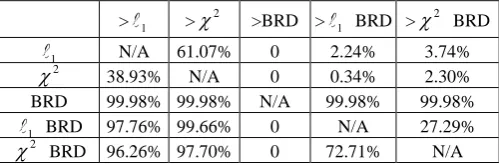
u v, excluding (1,1), the values of eD for the BRD are always larger than those for other distances. This means that the BRD is more robust to homogeneous background noise than other distances. [image:11.595.173.423.512.595.2]This is because the BRDs embed bin correlation information which remains stable against background clutter.
Table 1. The results of comparison between different histogram distances for simulated homogeneous background noise: in each row one of the distances is compared with other distances
> 1 >2 >BRD > 1 BRD >2 BRD
1 N/A 61.07% 0 2.24% 3.74%
2
38.93% N/A 0 0.34% 2.30%
BRD 99.98% 99.98% N/A 99.98% 99.98%
1 BRD 97.76% 99.66% 0 N/A 27.29%
2
BRD 96.26% 97.70% 0 72.71% N/A
In real applications, the background clutter may include occlusion, and the background noise is often very
complex, influencing the values of a number of bins. So, we explore partial matching when the histograms are
randomly corrupted.
We assume that the background corrupts the foreground object randomly, e.g., with occlusion. Let the vector
1 2
( b b b b)
back h h hi hn
h be the histogram of the background, where n is the number of bins and is
a parameter controlling the influence of background information. We define the histogram hA of the foreground
1 2
1 1 1 1
A A A A A
i n
B A
back C
h h h h
h
h h h
h
(17)
Each bin value in hA and hback is randomly sampled from a uniform distribution over [0, 1]. Because in real
applications only a part of the histogram bins are strongly perturbed by background data, we randomly set some bin
values in hback to zero. Let r[0, 1] be the fraction of the bins influenced by background. When r=1, the
background contains all types of visual words and influences every bin in hA. Given
and r, each pair hA andback
h are randomly generated, and it is checked whether the inequality d(hA,hB)d(hA,hC) holds for distance d.
This process is repeated for a number of times, and the probability that the inequality holds is calculated and used as
a measure of the robustness of d. Many probabilities can be recorded when and r change.
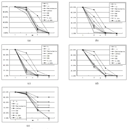
In the experiments, the number of bins was set to 100. Given a value of
and a value of r, 10000 sampleswere used to check whether d(hA,hB)d(hA,hC) holds, and then the probability of d(hA,hB)d(hA,hC) was
obtained. Fig. 2 shows the results for the 1 distance, the
2
distance, the Bhattacharyya distance, the Jeffrey
divergence, the EMD, the BRD, the 1 BRD, and the 2 BRD. The figure reveals the following useful points:
When =1, almost every histogram distance d yields a probability of 1 for d(hA,hB)d(hA,hC). This
means that when the background noise is small, all histogram distances give a correct classification.
When increases above 1, the performance for all the histogram distances falls rapidly. This shows that
large background noise has a strong negative effect on the accuracy of classification.
When r=1, the probability that d(hA,hB)d(hA,hC) is a maximum for each distance d. When r=0.4 or
0.6, the probability that d(hA,hB)d(hA,hC) is low. This is mainly due to the histogram normalization.
When r=1, all the bins of hB have larger values than the corresponding bins in hA. Then after
normalization, the distance between hA and hB decreases. When r=0.4, 40% of the bins in hB are
larger than the corresponding bins in hA and the rest have the same values as the corresponding bins in
A
h . After normalization, the 60% unchanged bins in hB are decreased and the 40% increased bins may
be increased or decreased. The result is that the distance between hA and hB is relatively large and
matching the histograms becomes less accurate. This situation is the most common in real applications,
because the background usually does not contain all the visual words of the foreground object.
The 1 BRD and the 2 BRD are significantly more accurate than all other distances. This result is
different from the results for the homogeneous background. This is because when the background corrupts
distances.
The different histogram distances have their own characteristics. For example, the BRD is robust to
homogenous background noise and the 2 BRD is robust to random background noise. No distance
measure can outperform all its competitors in all cases.
(a) (b)
(c) (d)
[image:13.595.90.511.144.566.2](e)
Fig. 2. The probabilities that d(hA,hB)d(hA,hC) for each histogram distance d, given random histogram corruption for a range of rand : (a) r=0.2; (b) r=0.4; (c) r=0.6; (d) r=0.8; (e) r=1. The x-coordinate indicates the values of , and the y-coordinate indicates the probabilities expressed as percentages.
4.2. Synthetic background images
From a real image dataset which consists of object images and background images, object images and
foreground images are selected and combined to produce synthetic images in the following two ways:
The background image is placed onto the foreground image such that the foreground object is partly
occluded by the background image.
The foreground object image is placed randomly onto the background image, and then the background
The histogram hA of each foreground image and the histogram hB of each synthetic image are constructed. The
reference histogram hC is set to the average histogram of all the foreground images. We calculate the probability
that d(hA,hB)d(hA,hC) for each distance function d using a large number of synthetic images. This probability
is used to measure the robustness of d.
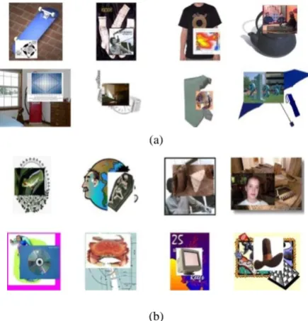
In the simulation, we selected 320 object images with 16 categories from the Caltech256 dataset [12], where
each category consists of 20 images and 467 background images. Each synthetic image was obtained by randomly
combining a foreground image and a background image from the dataset. Half of the synthetic images were obtained
by placing the background image onto the foreground image, as shown in Fig. 3 (a). The image size ratio of the
background image to the foreground object image was randomly chosen from [0.1, 0.3]. The foreground object
image was fixed, and the background image was resized according to and randomly placed onto the foreground
image. The limited range for ensures that there are no large occlusions. Half of the synthetic images were
obtained by randomly placing the foreground object image onto the background image, as shown in Fig. 3 (b). The
ratio was randomly chosen from [1.5, 4] to avoid too large clutter.
(a)
[image:14.595.187.405.356.583.2](b)
Fig. 3. Examples of synthetic images: (a) the foreground image is occluded by the background image; (b) the foreground image is placed randomly onto the background image.
For each foreground image, we repeated the above synthetic process 100 times to construct 100 synthetic
images. The classic bag-of-words model was used to map each image into a histogram. Scale invariant feature
transform (SIFT) features were extracted from images. The k-means method was employed to cluster the feature
vectors of the images into 200 clusters where each cluster corresponded to a visual word. For each image, the word
the closest to each feature component was found and the frequency of each word was counted to form the word
histogram. Then, the histogram hA of each foreground image, the histogram hB of each synthetic image, and the
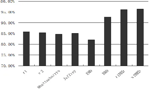
was calculated using the synthetic images. The results are shown in Fig. 4. It is seen that the 2 BRD has the most
accurate results, and the 1 BRD has accuracy close to the
2
BRD. The BRDs yield much more accurate results
than the 1 distance, the 2 distance, the Bhattacharyya distance, the Jeffrey divergence, and the EMD whose
[image:15.595.173.428.163.315.2]cost matrix was calculated using the 2 distances of codebook cluster centers.
Fig. 4. The probabilities of d(hA,hB)d(hA,hC) for each distance function d with a synthetic background experiment, where the x-coordinate indicates different histograms and the y-coordinate indicates the probabilities.
In the above three simulations, as reported in Sections 4.1 and 4.2, the robustness of the different histogram
distances to partial matching was thoroughly assessed. It is concluded that the BRDs are more robust to partial
matching than the traditional five distances functions: the 1 distance, the 2 distance, the Bhattacharyya distance, the Jeffrey divergence, and the EMD.
5. Kernel-Based Image Classification
To use bin ratio-based histogram distances (BRDs) for image classification [4, 7, 28, 44, 45], we combine
BRDs with the standard bag-of-words model. We follow the kernel-based framework in [43], i.e. we build the
kernels of the BRDs using the extended Gaussian kernels [5]:
1
, exp ,
K d
A
p q p q (19)
where d(p, q) is a squared distance between p and q which are histograms of two images, and A is a scaling
parameter that can be determined by cross-validation. In [43], it is shown that when A is the mean of all the distances
between samples, the 1 distance, the 2 distance, and the EMD empirically perform most accurately. It is shown
in our experiments that the BRD, the 1 BRD, and the 2 BRD perform empirically most accurately when A is set
to twice the mean of all the distances between samples. Currently, it is not known if BRDs-based kernels are Mercer
kernels. Nevertheless, in our experiments, these kernels have always produced positive definite Gram matrices. It is
noted that some widely used kernels, e.g. the EMD-kernel, are also not known to be Mercer kernels [43]. Some
non-Mercer kernels also work effectively in real applications [5].
classification results. Let
x
( ,
s s
1 2,
,
s
I)
, wheres
i(i=1,2,…,I) is the probability output of the i-th classifierand I is the number of classifiers. The logistic regression for information fusion is represented by:
( * )
1 ( )
1 w x
f x
e
(20)
where parameter vector w is estimated using the training samples. The label for each test sample is determined by the
output of the logistic regression. We use logistic regression to fuse the results of the 1 BRD, the 2 distance, the
Bhattacharyya distance, and the Jeffrey divergence for image classification.
We used the following seven benchmark datasets to test the performance of the BRDs and the logistic
regression-based histogram fusion for image and scene classification: the Scene-15 dataset [17], PASCAL VOC
2008 [7], PASCAL VOC 2005 [8], PASCAL VOC 2011, 17 Oxford Flowers [24], 102 Oxford Flowers [25], and
Caltech-256. In the following, we first give an initial description of the different datasets and their setups, then
provide a global synthesis of all the experiments, and finally describe the local analysis on individual datasets.
5.1. Datasets and setups
1) Scene-15 dataset: This dataset [17] is a combination of several earlier datasets [9, 17, 26]. It contains 4485
scene images from 15 categories, with 200 to 400 images per category. In [11], histogram intersection was used on
this dataset and a kernel codebook technique was used in comparison with standard codebook. For fair comparison,
we closely followed the experimental setup in [11]. For each image in this dataset, a SIFT descriptor was sampled on
a regular grid with space of eight pixels between neighboring grids. Each SIFT feature component was calculated on
a 16×16 patch. We applied the histogram intersection, the 2 distance, the 1 distance, and the proposed BRDs to the feature vectors of the images in this dataset. The dataset was randomly split into the training set and the test set. A
codebook vocabulary was generated using k-means on the training set. Normal codebook (hard assign) and kernel
codebook (allowing for code word uncertainty) were used respectively. For each type of codebook, the SVM was
employed for the kernels. For multi-class classification, we used the one-versus-all scheme in the Libsvm. Five-fold
cross-validation was applied to the training set to tune the parameters. The accuracy for classifying the test set was
calculated by averaging the accuracies of each category. The classification process was repeated for 10 rounds. The
average accuracies of the different distances over 10 rounds were reported.
2) PASCAL visual object classes (VOC) 2008: This dataset [7, 8, 23] consists of twenty object categories with
8465 images derived from the Internet. The backgrounds in the images are usually very complex. A single image
may contain multiple objects, and thus have multiple labels. The whole dataset has 2111 training images, 2221
validation images, and 4133 test images. Category labels are only released for the training and validation images.
The labels of the test images are unknown to all the users. The results on the test set must be sent to the PASCAL
training images were clustered using k-means to generate a vocabulary of 4000 words. The 1 BRD was used to
measure histogram distances. The extended Gaussian kernel and the SRKDA method in [3] were used to classify
images. The parameters were estimated on the validation set and then used on the test set.
3) PASCAL VOC 2005: We tested our method on the difficult classification test set (test 2) in the PASCAL
VOC 2005 dataset [8]. This test set is similar to PASCAL VOC 2008, but it only contains the following four
categories: motorbike, bicycle, car, and persons. There are 1543 images in the test set. An image may include persons
and a motorbike, and thus may have multiple labels. The best score in the competition to classify the images in the
test set was achieved by Zhang and Schmid [8] using the 2 distance with an extended Gaussian kernel. Later, Zhang et al. [43] obtained a similar result using the EMD distance. We followed Zhang and Schmid’s experimental
setup in [8]. The Harris-Laplace detector and the SIFT descriptor were used to extract features. We obtained 1000
visual words by clustering the training samples using k-means. For fair comparison, the standard codebook was
employed instead of the kernel codebook. We used the 1 BRD instead of the 2 distance in [8]. As in [8], the extended Gaussian kernel and the SVM classifier [4] were used. The parameters of the SVM were determined using
two-fold cross-validation on the training set.
4) PASCAL VOC 2011: We used the 2011 version of the PASCAL VOC classification dataset to make the
comparison. The PASCAL VOC 2012 classification dataset is the same as that used in 2011. No new data have been
added. In the dataset there are 10994 images in 20 classes. The classification results must be uploaded to the
PASCAL official website to obtain the information about their accuracy. We followed the experimental setup of the
winner of the PASCAL VOC 2011 classification challenge. For each image, SIFT, LBP (Local Binary Pattern), and
HOG features were extracted using dense sampling and the detector of points of interest. The features were then
aggregated into the holistic Bag-of-Words (BoW) image representations. Various patch features were extracted using
multiple image segmentations to form the image-level BoW representations. The detection features were obtained
using the deformable part model for different object classes. The resulting detection kernel was combined with the
visual feature kernel by weighted summation. Lasso prediction, the SVM, and the regression classifier were
combined into one classifier. Kernel regression was utilized to fuse all the confidences from these three classifiers.
5) 17 Oxford Flowers: This dataset [24] contains images from 17 flower categories. There are 80 images per
category. For each category, 40 images were used for training, 20 images for validation and 20 images for testing
[24]. We used the same experimental setup as for PASCAL 2008 except that we used the standard SVM instead of
the SRKDA. Thirty channels of features were used and combined by averaging the histogram distances of each
channel. For each feature, a kernel codebook of 4000 code words was used. We classified the images in this dataset
in three independent experiments and reported the average accuracy and variance.
6) 102 Oxford Flowers: This dataset [25] contains 8189 images from 102 flower categories with 40-250
images are the test images. We used the same experimental setup as for the above 17 Oxford flowers dataset, and this
setup is also the same as that used by the winners of PASCAL 2008, Tahir et al. [35]. Specifically, the feature vectors
of the training images were clustered to generate a vocabulary of 4000 words. Kernel codebook was used for vector
quantization. The parameters were estimated on the validation set and further used for the test set.
7) Caltech-256: The classical benchmarked Caltech-256 dataset, which was used to evaluate the robustness of
the BRDs to partial matching, was also used to evaluate image classification performance. As suggested by the
builders of the dataset, for each category 30 samples were selected for training, and 25 samples were selected for
testing. A dense sampling was used to generate local patches where each patch corresponds to a point of interest.
Then, each image patch was further represented by the RGB-SIFT descriptor. Three different image division modes
were used to represent each image: the whole image without subdivision (1x1), 4 image parts obtained by dividing
the image into 4 quarters (2x2) and 3 image parts obtained by dividing the image into three horizontal bands (1x3).
The lengths of the feature vectors for the three division modes are 2000, 6000, and 8000, respectively. A kernel was
constructed for each division mode, and the average of the three kernels was input to the SVM-based classifier. For
each image category, a vocabulary of 2000 words was generated by clustering and a binary classifier was designed.
A total of 256 binary classifiers were obtained.
[image:18.595.189.403.401.563.2]5.2. Global synthesis
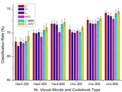
Fig. 5. Classification results for the various histogram distances on theScene-15 dataset over different vocabulary sizes and codebook types. The terms “Hard” and “Unc” refer to hard assignment and uncertain assignment.
Fig. 5 shows the results, on the Scene-15 dataset, of the 2 distance, the 1 distance, the BRD, the 2
BRD, the 1 BRD, and the histogram intersection with the following codebook sizes: 200, 400, and 800, and with
normal codebook (hard assign) or kernel codebook (code word uncertainty). Table 2 compares the classification
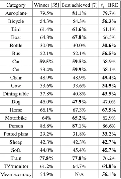
precision of our method on the test set of the PASCAL VOC 2008 datasetwith those of Tahir et al.’s method [35] and
with the highest classification precisions for each image category from all the competitors of PASCAL 2008. Table 3
compares the results, on the PASCAL VOC 2005 data, of our 1 BRD and logistic regression with the results of the
methods in [8, 21, 43], where the logistic regression fuses the 1 BRD, the 2 distance, the Bhattacharyya distance,
and the Jeffrey divergence. Table 4 shows the results, on the PASCAL VOC 2011 dataset, of the methods based on
the 1 BRD kernel, and the 2 distance kernel, the Bhattacharyya distance kernel, and the Jeffrey divergence
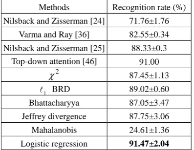
kernel, and the result of the winner of the challenge. Table 5 summarizes the recognition accuracies, on the 17
Oxford flowers dataset, of the 1 BRD-based method, the 2 distance-based method, the Bhattacharyya distance-based method, the Jeffrey divergence-based method, and the Mahalanobis distance-based method, the
top-down attention-based method [46], the excellent methods in [24, 25, 36], and the logistic regression-based
method. Table 6 shows the recognition rates, on the 102 Oxford flower dataset, of the 1 BRD-based method, the
methods based on the competing histogram distances, the logistic regression-based method, and Nilsback and
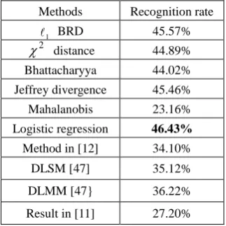
Zisserman’s method [25]. Table 7 shows the results, on the Caltech256 dataset, of the 1 BRD, the competing
histogram distances, the logistic regression, the method in [12], the method based on the dictionary learning on
single manifold (DLSM) in [47], the method based on the dictionary learning on multiple manifolds (DLMM) in
[47], and the method in [11]. The experimental setups for the different histogram distances are exactly the same to
avoid bias. From these tables and figure, the following global properties are revealed:
The results of the 1 BRD are more accurate than or comparable to the state-of-the-art results in all the
datasets.
Our 1 BRD yields more accurate results than the 2 distance, the Bhattacharyya distance, the Jeffrey
divergence, and the Mahalanobis distance.
The logistic regression-based information fusion overall improves the classification accuracies of the
individual histogram distances. So, there is room for improvement of the accuracy of the 1 BRD.
The Mahalanobis distance yields much less accurate results. This is because the feature vectors are very
sparse, and the covariance matrix is unable to describe the distribution of the features.
The results clearly show the effectiveness of the 1 BRD.
5.3. Local analysis on individual datasets
1) Scene-15 dataset: On this dataset, the results from our re-implementation of the histogram intersection are
close to the results in [11]. The performance of the BRD by itself is comparable to the performance of histogram
intersection, although the BRD is sensitive to small noise. This indicates that bin-ratios contain rich discriminative
information. The 1 BRD yields the largest average classification rates over each vocabulary size and each
codebook type. This demonstrates the effectiveness of the combination of the BRD and the 1 distance. The BRD
and the 2 BRD are robust to different types of background, but for complex backgrounds in the set of real images,
2) PASCAL VOC 2008: It is shown that the 1 BRD outperforms the winner’s method in 14 out of 20
categories, and it has a better average performance. Since we strictly followed the winner’s method except for the
histogram distance, the results on the PASCAL 2008 dataset clearly demonstrate the superiority of the proposed bin
ratio-based distance. In 11 out of the 20 categories, the precisions of our method are higher than the best precisions
obtained by all the competitors. In 9 out of 20 categories, the 1 BRD did not achieve the best results. This is
because the best results for different image categories may be due to particular choices of features and classification
strategies, and the features used in our method and the assumption of the BRD may not be most suitable for these 9
[image:20.595.193.404.261.572.2]categories.
Table 2. Precisions of the winner’s method, the best precisions per category among all competitors of PASCAL 2008, and the precisions of our method on the test set of PASCAL 2008.
Category Winner [35] Best achieved [7] 1 BRD
Aeroplane 79.5% 81.1% 79.7%
Bicycle 54.3% 54.3% 56.3%
Bird 61.4% 61.6% 61.1%
Boat 64.8% 67.8% 66.5%
Bottle 30.0% 30.0% 30.6%
Bus 52.1% 52.1% 56.5%
Car 59.5% 59.5% 58.9%
Cat 59.4% 59.9% 58.1%
Chair 48.9% 48.9% 49.4%
Cow 33.6% 33.6% 34.9%
Dining table 37.8% 40.8% 43.5%
Dog 46.0% 47.9% 47.0%
Horse 66.1% 67.3% 67.5%
Motorbike 64% 65.2% 62.9%
Person 86.8% 87.1% 86.6%
Potted plant 29.2% 31.8% 33.2%
Sheep 42.3% 42.3% 42.7%
Sofa 44.0% 45.4% 45.7%
Train 77.8% 77.8% 76.2%
TV/monitor 61.2% 64.7% 64.8%
Mean accuracy 54.9% N/A 56.1%
Table 3. Correct classification rates at equal error rates on test set 2 in the PASCAL challenge 2005
Motor Bike Person Car Average
Winner [8] 79.8% 72.8% 71.9% 72% 74.1%
Winner (EMD) [43] 79.7% 68.1% 75.3% 74.1% 74.3% Ling and Soatto [21] 76.9% 70.1% 72.5% 78.4% 74.5%
1 BRD 79.1% 75.4% 73.9% 78.2% 76.7%
Bhattacharyya 75.3% 74.1% 72.6% 78.5% 75.1%
Jeffrey divergence 76.5% 73.5% 74.3% 74.2% 74.6%
Mahalanobis 41.3% 71.9% 62.2% 75.5% 62.7%
Logistic regression 77.3% 72.5% 75.5% 83.2% 77.1%
[image:20.595.178.418.599.727.2]proposed 1 BRD is not sensitive to different image categories. In contrast with Ling and Soatto’s method [21] in
which the spatial co-occurrence statistics are considered in the feature extraction stage, the 1 BRD obtains more
accurate results in the categories of Motor, Bike, and Person by more than 1.4%, but very slightly less accurate
results on the category of Car with a decrease of only 0.2%. The 1 BRD improves on the average classification of
Ling and Soatto’s method by 2.2%. This indicates that our method is effective to considercorrelations between pairs
of histogram bins. It is noted that the 1 BRD does not yield the most accurate results for some image categories.
One of the reasons is that if the noise completely destroys the bin ratio relations in the histograms of the images in
the same category, the 1 BRD may not be accurate enough to compute the distances between histograms.
4) PASCAL VOC 2011: Although many non-trivial adjustments [48] used by the winner cannot be duplicated
by us, the result of the 1 BRD-based method, which is more accurate than the results of the 2 distance-based
method, the Bhattacharyya distance-based method, and the Jeffrey divergence-based method, is still comparable to
[image:21.595.216.379.355.441.2]the winning result of the PASCAL VOC 2011 challenge.
Table 4. The average precisions of different methods on the PASCAL VOC 2011 dataset
Methods Recognition rate
1 BRD 77.17%
2
distance 76.82%
Bhattacharyya 72.50%
Jeffrey divergence 76.61%
Winner 78.56%
5) 17 Oxford Flowers: The 1 BRD yields a larger average recognition rate and a smaller standard deviation
than the method in [25], which is in turn more accurate than the methods in [24, 36]. The result of the top-down
attention-based method [46] is slightly higher than that of our BRD-based method. This is because, in the top-down
attention-based method, the hue features were included in the process of producing bag of words based on the SIFT
features. When the logistic regression was used to fuse different histogram distances, an average recognition rate
which is larger than that of the top-down attention-based method was obtained.
Table 5. The average recognition rates of different methods on the 17 Oxford flowers dataset
Methods Recognition rate (%)
Nilsback and Zisserman [24] 71.76±1.76
Varma and Ray [36] 82.55±0.34
Nilsback and Zisserman [25] 88.33±0.3
Top-down attention [46] 91.00
2
87.45±1.13
1 BRD 89.02±0.60
Bhattacharyya 87.05±3.47
Jeffrey divergence 87.75±3.06
Mahalanobis 24.61±1.36
[image:21.595.199.398.609.763.2]6) 102 Oxford Flowers: It is seen that our 1 BRD-based method yields a higher recognition rate than the
method of Nilsback and Zisserman who produced the dataset. Logistic regression explicitly improves the
classification accuracies of the individual distances.
Table 6. The average recognition rates of different methods on the 102 Oxford flower dataset.
Methods Recognition rate
Nilsback and Zisserman [25] 72.80%
2
79.68%
1 BRD 80.45%
Bhattacharyya 79.01%
Jeffrey divergence 79.43%
Mahalanobis 17.30%
Logistic regression 81.60%
7) Caltech-256: The result of the 1 BRD is comparable to the recently published results. The logistic
[image:22.595.217.379.341.503.2]regression yields the most accurate result.
Table 7. The average recognition rates of different methods on the Caltech-256 dataset
Methods Recognition rate
1 BRD 45.57%
2
distance 44.89%
Bhattacharyya 44.02%
Jeffrey divergence 45.46%
Mahalanobis 23.16%
Logistic regression 46.43%
Method in [12] 34.10%
DLSM [47] 35.12%
DLMM [47} 36.22%
Result in [11] 27.20%
6. Conclusion
In this paper, we have proposed a group of bin ratio-based histogram distances, i.e., the BRD, the 1 BRD, and
the 2
BRD. These are new types of histogram distance, namely intra-cross-bin distances, while previous
histogram distances have been bin-to-bin distances or cross-bin distances. These BRDs contain the correlations
between pairs of histogram bins, while maintaining a linear computational complexity. They are robust to partial
matching and histogram normalization. The 1 BRD and the 2
BRD can overcome the sensitiveness of the BRD
to small bin values or noise. The robustness of the BRDs to partial matching is demonstrated using synthetic datasets.
We have compared BRDs experimentally with several state-of-the-art histogram distance measures on seven
benchmark datasets for image classification. Among these histogram distances, the 1 BRD overall generates the
![Fig. 1. An example of the effects of partial matching on the distances between histograms: (a), (b) and (c) show three histograms before normalization, where histograms in (a), (b), and (c) are [1, 3, 14, 1, 0], [1, 3, 14, 1, 25], and [10, 10, 10, 10, 10],](https://thumb-us.123doks.com/thumbv2/123dok_us/8872744.942668/4.595.132.463.449.658/example-effects-matching-distances-histograms-histograms-normalization-histograms.webp)