Multiple path Quantum Interference Effects in a Double Aharonov Bohm Interferometer

N A N O I D E A S

Multiple-path Quantum Interference Effects

in a Double-Aharonov-Bohm Interferometer

X. F. Yang•_{Y. S. Liu}

Received: 10 March 2010 / Accepted: 4 May 2010 / Published online: 22 May 2010 The Author(s) 2010. This article is published with open access at Springerlink.com

Abstract We investigate quantum interference effects in a double-Aharonov-Bohm (AB) interferometer consisting of five quantum dots sandwiched between two metallic elec-trodes in the case of symmetric dot-electrode couplings by the use of the Green’s function equation of motion method. The analytical expression for the linear conductance at zero temperature is derived to interpret numerical results. A three-peak structure in the linear conductance spectrum may evolve into a double-peak structure, and two Fano dips (zero conductance points) may appear in the quantum system when the energy levels of quantum dots in arms are not aligned with one another. The AB oscillation for the mag-netic flux threading the double-AB interferometer is also investigated in this paper. Our results show the period of AB oscillation can be converted from 2ptopby controlling the difference of the magnetic fluxes threading the two quantum rings.

Keywords Aharonov-Bohm interferometer

Fano effectsQuantum dotsTransport properties

Thanks to rapid developments in the fabrication and self-assembly techniques, the electrical transport through nanoscale quantum systems such as a single quantum dot, multiple quantum dots, atoms or molecules coupled to metallic electrodes has been an interesting subject in recent years [1–6]. In the nanoscale quantum systems, the elec-trical transport is ballistic, while the phase coherence of the

electrons is preserved. Especially, the quantum interference effects in an AB ring including a quantum dot have been reported [7]. The results showed that Fano effect with asymmetric parameters was a good probe to quantum interference effects in the nanoscale systems. The transport properties of a quantum ring consisting of two parallel-coupled quantum dots sandwiched between two metallic electrodes have been also studied theoretically and exper-imentally in the last few decades [7–22]. For example, an AB interferometer including two coupled quantum dots with each quantum dot inserted in each arm was presented, and an oscillating electric current was detected experi-mentally [8, 9]. Such a double-quantum-dot model con-sisting of the parallel-coupled double-dot system has been studied extensively in some previous theoretical works [13–18]. When the interdot coupling is considered, a bonding molecular state and an antibonding molecular state are developed. A swap effect can be found in the quantum system by tuning the magnetic flux threading the quantum ring, which may be used in the future quantum computa-tions [15].

Recently, the transport properties of multi-parallel-cou-pled quantum dots have attracted considerable attention due to their potential applications and abounding physics [23–31]. Zeng et al. studied the AB effects in a quantum ring consisting of four quantum dots sandwiched between two metallic electrodes, and a Fano dip is developed when the energy levels of quantum dots in two arms are mis-matched [23]. Guevara et al. offered a quantum model describing multi-parallel-coupled quantum-dot molecule, and Fano effects in the quantum system were studied in detail [24]. More recently, Li et al. studied the electrical transport through a triple-arm AB interferometer consisting of three parallel quantum dots with electron-electron interactions under an applied electric field [25].

X. F. YangY. S. Liu (&)

Jiangsu Laboratory of Advanced Functional Materials, and College of Physics and Engineering, Changshu Institute of Technology, 215500 Changshu, China

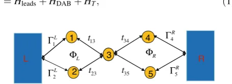
In this work, we study the quantum interference effects in a double-Aharonov-Bohm interferometer consisting of five quantum dots sandwiched between two metallic elec-trodes as shown in Fig.1. The left quantum ring consisting of the quantum dot 1, the quantum dot 2, quantum dot 3 and the left metallic electrode encloses the magnetic flux UL. The right ring consisting of the quantum dot 3, the quantum dot 4, the quantum dot 5, and the right metallic electrode encloses the magnetic flux UR. Two quantum rings are connected together by the quantum dot 3. For simplicity, we consider that only one energy level exists in each quantum dot, and the energy levels of all quantum dots can be tuned by the voltages applied on the quantum dots. In this work, we studied in detail the quantum inter-ference effects in the double-quantum-ring structure in the case of symmetric dot-electrode couplings. The results show that the linear conductance peaks at zero temperature can be effectively tuned by using the intermediate quantum dot 3. As the energy level of the quantum dot 3 changes, a three-peak structure may evolve into a two-peak structure in the linear conductance spectrum. When the energy levels of quantum dots in arms are not aligned with one another, two Fano dips may appear in the double-quantum-ring device. Two Fano peaks can be effectively modified by tuning the energy level of quantum dot 3. The AB oscil-lation for magnetic flux is also studied in this work. Our results show that the AB oscillating behavior depends strongly on the difference between the magnetic fluxes threading the left and right rings. In addition to the general AB oscillation with 2p-period, an AB oscillation with

p-period can be developed when the difference between the two magnetic fluxes is (2n ?1)p(n =0, 1, 2,…).

Model and Methods

The parallel-coupled quantum-dot structure that we con-sider is illustrated in Fig.1. For simplicity, the interdot and intradot coulomb interactions are neglected, and the total Hamiltonian describing the quantum system is written as

H¼HleadsþHDABþHT; ð1Þ

where the first term Hleads in Eq. (1) describes the left

and right electrodes in the noninteracting electron approximation

Hleads¼ X

a¼L;R;k

akayakaak; ð2Þ

whereay_akðaakÞdenotes the creation(annihilation) operator for an electron with energyeakand momentumkin electrode a. The second term in Eq. (1) describes the dynamics of the five parallel-coupled quantum dots, which can be modeled by using the following five-site Hamiltonian

HDAB¼ X5

j¼1

jdyjdj ðt13ei/L=4d1yd3þt23ei/L=4dy2d3

þt34ei/R=4dy3d4þt35ei/R=4dy3d5þh:c:Þ; ð3Þ

where dy_jðdjÞ creates (annihilates) an electron with the energyej in the jth quantum dot, and the AB phase /a¼ 2pUa=U0ða¼L;RÞ and the flux quantum U0 ¼h=e. tij

describes the interdot tunneling coupling between the doti

and dot j, for convenience, which is regarded as a real number. The third term in Eq. (1) describing the tunneling coupling between the quantum dots and the electrodes is divided into two parts

HT¼HTLþH R

T: ð4Þ

H_Ta describes the tunneling coupling between the isolated quantum dots and the electrodea

H_TL¼X

k

½ðVL1dy1þVL2d2yÞaLkþH:c:; ð5Þ

and

H_TR¼X

k

½ðVR4d y 4þVR5d

y

5ÞaRkþH:c:: ð6Þ

A phase factor is attached to Vaj in the presence of the

magnetic flux, and they can be written asVL1¼ jVL1jei/L=4,

VL2¼ jVL2jei/L=4, VR4 ¼ jVR4jei/R=4, VR5¼ jVR5jei/R=4.

In order to study the transport through the double-quantum ring, we need know the retarded (advanced) Green’s function

Gr_ijðaÞðÞ. The retarded Green’s function is defined as

Gr_ijðÞ ¼dijdyj r

ði;j¼1;2;3;4;5Þ: ð7Þ Applying the equation of motion method, we obtain a series of equations [32],

ð1ÞGr11ðÞ ¼1t13ei/L=4Gr31ðÞ

þX

k

VL1aLkjd1y

r ;

ð8Þ

ð2ÞGr22ðÞ ¼1t23ei/L=4Gr32ðÞ

þX

k

VL2aLkjd2y

r

; ð

9Þ R

1 L

Γ 1 t13 t34 4 Γ4

ΦL 3 ΦR _R

L t t R

2

Γ 2 23 35 5 Γ5 L

Fig. 1 Schematic plot of a double-Aharonov-Bohm interferometer consisting of five quantum dots sandwiched between two metallic electrodes. Theleft ringencloses a magnetic fluxUL, and theright

ð3ÞGr33ðÞ ¼1t13ei/L=4Gr13ðÞ t23ei/L=4Gr32ðÞ t34ei/R=4Gr43ðÞ t35ei/R=4Gr53ðÞ;ð10Þ ð4ÞGr44ðÞ ¼ 1t34ei/R=4Gr34ðÞ

þX

k

VR4aRkjdy4

r

; ð

11Þ

ð5ÞGr55ðÞ ¼ 1t35ei/R=4Gr35ðÞ

þX

k

VR5aRkjdy5

r

: ð

12Þ

Four new Green’s functions arising from the tunneling couplings between the quantum dots and metallic electrodes appear in the above Eqs. (8–9) and Eqs. (11– 12), and they are

ðLkÞ aLkjd1y

r ¼V

L1G

r

11ðÞ þV

L2G

r

21ðÞ; ð13Þ ðLkÞ aLkjd₂yr ¼V

L1G

r

12ðÞ þV

L2G

r

22ðÞ; ð14Þ ðRkÞ aRkjdy4

r ¼V

R4G

r

44ðÞ þV

R5G

r

54ðÞ; ð15Þ ðRkÞ aRkjdy₅r¼V

R4G

r

45ðÞ þV

R5G

r

55ðÞ: ð16Þ

Using the above Eqs. (8–16), the retarded Green’s functionGrcan be calculated by the following 5 95 matrix

where gj¼jþ2iC

a

j and Caj ¼

P

kjVajj

2

2pdðak) (j=1, 2 for a=L; j=4, 5 for a =R). The advanced Green’s functionGais obtained by the relationGa_ij¼Gr_ji. The linear conductance of the double quantum ring at zero temperature can be calculated by the Landauer Formula [32],

r¼2e 2

h Tr½C

L_Gr

CRGa: ð18Þ

The linewidth matricesCL_andCR _{are given}

CL_¼

CL₁

ffiffiffiffiffiffiffiffiffiffiffi

CL₁CL₂

q

ei/L=2 _{0 0 0} ffiffiffiffiffiffiffiffiffiffiffi

CL1C

L

2 q

ei/L=2 _CL

2 0 0 0

0 0 0 0 0

0 0 0 0 0

0 0 0 0 0

0 B B B B B B @ 1 C C C C C C A

ð19Þ

and

CR _¼

0 0 0 0 0

0 0 0 0 0

0 0 0 0 0

0 0 0 CR4

ffiffiffiffiffiffiffiffiffiffiffiffi

CR4C

R

5 q

ei/R=2

0 0 0

ffiffiffiffiffiffiffiffiffiffiffiffi

CR4C

R

5 q

ei/R=2 _CR 5 0 B B B B B B @ 1 C C C C C C A :

ð20Þ

In the case of the symmetrical dot-electrode tunneling couplings ðCL1¼C

L

2 ¼C

R

4 ¼C

R

5 ¼CÞ, the linear

conduc-tance has the following form,

r¼2e

2_C2

h

_X

m¼1;2;n¼4;5

jGr_mnj2þ2Re

Gr₁₄ Ga₅₁ei/2Rþ_Ga

42e

i/L

2

þGr25 G a 42e

i/R 2þ_Ga

51e i/L

2

þGr25G a 41e

i/_þGr 24G

a 51e

iD₂/

;

ð21Þ

where/¼ð/Lþ/RÞ=2 andD/¼ð/L/RÞ. From the above equation, we note that the linear conductance includes the contributions from four different electron tunneling paths (1?3? 4, 1?3?5, 2?3?4;2?3?5) and interference terms among them. Equation (21) is also written as:

r ¼ 2e 2_C2

h jG

r

14e i

4ð/Lþ/RÞþ_Gr 15e

i

4ð/R/LÞþ_Gr 24e

i

4ð/L/RÞ

þGr₂₅e4ið/Lþ/RÞj2_: ð₂₂Þ

Results and Discussion

In this section, the dependence of the linear conductancer

on system parameters is discussed numerically and ana-lytically. The coupling strength between the quantum dots and the metallic electrodes C is taken as the energy unit. Through this paper, all energy levels in quantum dots, tunneling couplings and Fermi energy are measured byC. Without Magnetic Flux

We first study the linear transport properties of the double-AB interferometer consisting of five parallel-coupled Gr¼

g1 ₂i ffiffiffiffiffiffiffiffiffiffiffi

CL₁CL₂

q

ei/L=2 t₁₃ei/L=4 0 0

i

2 ffiffiffiffiffiffiffiffiffiffiffi

CL₁CL₂

q

ei/L=2 _g

2 t23ei/L=4 0 0

t13ei/L=4 t23ei/L=4 3 t34ei/R=4 t35ei/R=4

0 0 t34ei/R=4 g4 2i

ffiffiffiffiffiffiffiffiffiffiffiffi

CR4C

R

5 q

ei/R=2

0 0 t35ei/R=4 ₂i

ffiffiffiffiffiffiffiffiffiffiffiffi

CR4C

R

5 q

ei/R=2 _g5 0 B B B B B B B B B @ 1 C C C C C C C C C A 1

quantum dots with the same energy levels (ej=0,

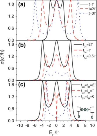
j=1, 2, 3, 4, 5) in the absence of the magnetic fluxes (/L=/R=0). Figure2a shows the linear conductancer

of the double-quantum-ring structure as a function of the Fermi level EF in the case of symmetrical interdot

tun-neling couplings. The same interdot tuntun-neling coupling strengths are chosen ast13 =t23 =t34 =t35 =t. There are

total five molecular states in center five-dot quantum sys-tem, but three molecular states of which with zero energy are degenerate. Other two molecular states are located at -2t and 2t, respectively. So we find that there are three resonance peaks withr =2e2/happearing at 0, 2tand-2t, respectively. With t increasing, the position of the center conductance peak has no changing, while the other two conductance peaks move in the opposite direction as shown in Fig.2a. In Fig.2b and c, we display the linear con-ductanceras a function of the Fermi energyEFin the case

of asymmetrical interdot tunneling couplings. In Fig.2b, we assume the interdot tunneling coupling strengths as

t13¼t23¼2C and t34=t35. In this case, three

conduc-tance peaks are located at 0, ffiffiffiffiffiffiffiffiffiffiffiffiffiffiffiffiffiffiffiffiffiffi2ðt2 13þt234Þ p

, and

ffiffiffiffiffiffiffiffiffiffiffiffiffiffiffiffiffiffiffiffiffiffi2ðt2 13þt

2 34Þ p

, respectively. As t34 decreases, the

con-ductance peaks are suppressed and become narrower as shown in Fig.2b. In Fig. 2c, we examine the transport properties of the double-quantum-ring structure by tuning

t23andt34. Here we fix the interdot tunneling couplingst13

andt35at 2C. A Fano dip (zero conductance point) appears

at EF=0 when t23 (t34) is different from t13(t35). The

behind reason is the destructive interference effects

between the electron waves directly transmitting through the three coupled quantum dots in series and side-coupled quantum dots (see the inset in Fig.2c). As t23 and t34

decrease, a three-peak structure in the linear conductance spectrum evolves into the four-peak structure. When

t23 =t34 =0, the quantum device becomes a three

quan-tum-dot array sandwiched between two metallic electrodes with side-coupled quantum dots as shown in the inset of Fig.2c. The Fano dip is located at the energy levels of the side-coupled quantum dots (e2=e4=0). It is noted that

two peaks become closer and narrower as t23 and t34

decrease. When t23=t34=0, the two conductance peaks

are located atpffiffiffi2t13ðt35Þ.

Figure3 displays the linear conductance r as a func-tion of EF when the energy level of the third quantum

dot e3 is not aligned with those of the other four

quan-tum dots. Five molecular states appear at 0;0;0;1 2

3

ffiffiffiffiffiffiffiffiffiffiffiffiffiffiffiffiffiffiffiffi

2 3þ16C

2

q

;1 2 3þ

ffiffiffiffiffiffiffiffiffiffiffiffiffiffiffiffiffiffiffiffi

2 3þ16C

2

q

, respectively. Whene3=0, three conductance peaks withr=2e2/hare

centered at 0, 2C and2C, respectively. The linear con-ductanceras a function ofEFunder the different values of e3 is plotted in Fig.3a and b. The left two conductance

peaks evolve into a single conductance peak, and the right conductance peak moves in the right direction in the case of e3[0. We also find the height of the left conductance

peak is suppressed. In the case ofe3\0, the situation is in

inverse. The right two conductance peaks evolve into a single conductance peak, and the height of the conductance peak is suppressed. The left conductance peak moves in the left direction, and the height of the conductance peak has no changing. In order to explore the dependence of the linear conductance on the energy level of the intermediate

0.0 0.6 1.2 1.8

0.0 0.6 1.2 1.8

-10 -8 -6 -4 -2 0 2 4 6 8 10 0.0

0.6 1.2 1.8 (c)

(b)

t=Γ

t=2Γ

t=3Γ

(a)

t 34=2Γ t

34=Γ t

34=0.5Γ

σ

(e

2 /h)

t 23=t34=2Γ t₂₃=t₃₄=Γ

t₂₃=t₃₄=0

E_F/Γ

Fig. 2 Linear conductance r as a function of EF under different interdot tunneling couplings. The energy levels of the quantum dots are chosen ase1=e2=e3=e4=e5=0

0.0 0.6 1.2 1.8

-8 -6 -4 -2 0 2 4 6 8

0.0 0.6 1.2

1.8 _(b) ε₃=0

ε₃=-Γ

ε₃=-2Γ

ε₃=-3Γ

ε₃=-4Γ

ε3=0

ε3=Γ

ε3=2Γ

ε3=3Γ

ε3=4Γ

σ

(e

2 /h)

(a)

E_F/Γ

Fig. 3 Linear conductanceras a function of the Fermi energy level

quantum dot 3, we plot the linear conductance as a function of e3under several different interdot couplings in Fig.4.

With e3 increasing, the linear conductance first increases

and reaches the maximum value at the certain valuee3m.

When the interdot couplings become small, e3m moves

toward the Fermi energy. Once the interdot couplings are enough small, the resonant conductance peak is almost pined atEF. The transport properties of the

double-quan-tum ring are similar with these of a single quandouble-quan-tum dot coupled straightly to metallic electrodes.

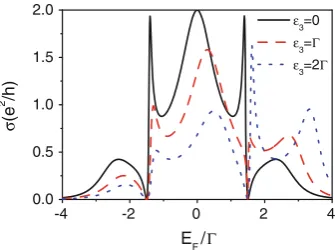
In Fig.5, we study the transport properties of the dou-ble-quantum ring when the quantum-dot levels are not aligned with one another. The same interdot coupling strengths (t13=t23=t34=t35=t=C) are considered,

and the energy levels of quantum dots parameters are chosen as 1¼ 2C; 2¼ C, 4¼C and 5¼2C,

respectively. Since the degenerate states are opened in this case, five conductance peaks appear in the linear conduc-tance spectrum. The linear conducconduc-tancerconsists of three Breit-Wigner peaks and two sharp asymmetric Fano peaks. A Fano dip happens at 1þ2

2 , while the other Fano dip

appears at4þ5

2 . The numerical results may be explained by

using Eq. (21). The linear conductance in the absence of magnetic flux can be written as

r¼2e 2_C2

h jG

r

14þG

r

24þG

r

25þG

r

15j 2

: ð23Þ

Using Eq. (17), we arrive at

r¼2e 2_C2

h t4_ð2E

F12Þ 2

ð2EF45Þ 2

jdet½Gr1_j2 : ð24Þ From the above equation, we see clearlyr=0 forEF ¼ 1þ2

2 or EF ¼

4þ5

2 . The linear conductance spectrum has

mirror symmetry around e3 in the case of e3=0. With

increasinge3, the mirror symmetry is broken. The left Fano

peak is suppressed, while the right Fano peak is firstly suppressed, then it is enhanced.

With Magnetic Flux

The periodic oscillation in the linear conductance for the magnetic flux is key features when the phase coherence of the electrons is preserved. In this section, we start with the study of dependence of the linear conductance on the magnetic fluxes through the double-quantum ring. The dependence of the linear conductance on the Fermi energy in the presence of the same magnetic flux through the left and right rings (/L=/R=/) is shown in Fig.6. The

same interdot tunneling couplings ðt13¼t23¼t34 ¼t35 ¼

CÞ and the same quantum-dot energy levels e1= e2= e3=e4=e5=e0=0 are considered. When the magnetic

flux/is presented, a Fano dip is developed when the Fermi energy is aligned withe0. With/increasing, the three-peak

structure disappears, while a four-peak structure in the linear conductance spectrum appears. When the magnetic fluxes are further increased, the four-peak structure evolves into a double-peak structure. The results may be explained by the following expressions. After some algebra, we derive the linear conductance r in the presence of the magnetic flux as the following analytical form

-8 -6 -4 -2 0 2 4 6 8

0.0 0.5 1.0 1.5 2.0

t

13=t23=t34=t35=0.2Γ t

13=t23=t34=t35=0.5Γ t

13=t23=t34=t35=Γ

σ

(e

2 /h)

ε₃/Γ

Fig. 4 Linear conductanceras a function of the energy level of the quantum dot 3 in the presence of different interdot tunneling coupling strengths. Other system parameters are chosen as in Fig.2

-4 -2 0 2 4

0.0 0.5 1.0 1.5 2.0

ε3=0

ε3=Γ

ε3=2Γ

σ

(e

2 /h)

E_F/Γ

Fig. 5 Linear conductanceras a function of the Fermi energyEF under several different values of the quantum dot 3. Other quantum-dot energy levels are chosen as 1¼ 2C, 2¼ C, 4¼C and 5¼2C, respectively

rðEF;/Þ ¼ 2e2C2

h

4E2_FC4_{½1þcosð/Þ}2

From the above equation, we see clearly that the linear conductance disappears whenEF=0, and four molecular

states are located around 2C and pffiffiffiffiffiffiffiffiffiffiffiffiffiffiffiffiffiffiffiffiffiffiffiffi22cosð/ÞC, respectively. With / increasing, the two middle conduc-tance peaks are suppressed obviously, while the outside conductance peaks become shaper as shown in Fig.6.

When / approaches p, we can obtain an approximate formula for the linear conductance

r’2e 2_C2

h

4E2

FC

4 d1 ðE2

FþC

2_Þ½2E2

FðE2F4C

2_Þ2

þd2; ð26Þ

whered1andd2represent two small quantities. Equation (26)

shows two narrower conductance peaks are centered at2C as shown in Fig.6. When/=np(nis odd number), the linear conductance disappears everywhere for any value ofEF.

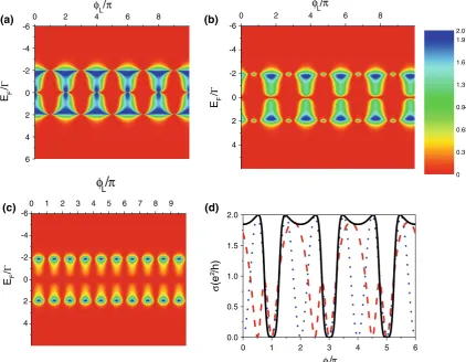
Figure7 shows the images of the linear conductancer

as functions of /L and the Fermi energy EF. The same

interdot couplings and same quantum-dot levels are con-sidered. D/¼/L/R denotes the difference between magnetic fluxes through the left quantum ring and right quantum ring. When D/6¼ ð2nþ1Þp, a general 2p -peri-odic AB oscillation for/Lis obtained as shown in Fig.7a and b. WhenD/¼ ð2nþ1Þp, ap-periodic AB oscillation appears in the quantum system as shown in Fig.7c. The above results can be explained as following expressions. When the magnetic fluxes through the double-quantum ring are considered, using Eq. (24), we arrive at

-4 -2 0 2 4

0.0 0.6 1.2

1.8 φ=0.1π

φ=0.4π

φ=0.8π

φ=π

σ

(e

2 /h)

E_F/Γ

Fig. 6 Linear conductanceras a function of the Fermi energyEF under several different magnetic fluxes threading theleftand right rings/L=/R=/

0 2 4 6 8 -6 -4 -2 0 2 4

0 8

-6

-4

-2

0

2

4

6

0 1 2 3 4 5 6 7 8 9

-6

-4

-2

0

2

4

φ

/

π

EF

/

Γ

2 4 6 0 2 4 6 8

-6

-4

-2

0

2

4

φ_L

/

EF

/

Γ

EF

/

Γ

φ_L/_π

(a) (b)

(c) (d)

0 0.31 0.63 0.94 1.3 1.6 1.9 2.0

0 1 2 3 4 5 6

0.0 0.5 1.0 1.5 2.0

σ

(e

2 /h

)

φ_L/π

Fig. 7 Images of the linear conductanceras functions of the fermi energy EF and /L for a D/¼0, b D/¼0:5p, and c D/¼p, respectively.dLinear conductanceras a function of magnetic flux

When /R/L¼D/¼p, the above equation can be simplified as

r¼2e 2_C2

h

2E2

FC

4_½1cosð2 /LÞ

ðE2

FþC

2_Þ½E2

FðE2F4C

2_Þ2

þC2ðE2

F2C

2_Þ2 : ð28Þ

So an AB oscillation with p-period is developed as shown in Fig.7c and d.

It is well known that an oscillating current in the AB interferometer has been detected experimentally [8,9]. For a single quantum ring consisting of two parallel-coupled quantum dots sandwiched between two metallic electrodes, 2p-periodic oscillation of the linear conductance r is reported in the pervious works [13]. The linear conduc-tanceras a function of/Lunder the different energy levels

in the quantum dot 3 or several different values of/R is shown in Fig.8. The Fermi energyEFis fixed at 0:2C, and

other system parameters are chosen as in Fig.6. The AB oscillation for /L in the presence of different energy

levels of the quantum dot 3 is potted in Fig.8a. Fore3=0,

a series of shaper resonant peaks appear at 2n

p(n =0, 1, 2…), and the linear conductance reaches a minimum (r=0) when /L approaches (2n?1)

p(n =0, 1, 2…). When the energy level in quantum dot 3 is not aligned with other quantum-dot levels, the single conductance peak around 2np splits into the two conduc-tance peaks. Withe3moving away from zero energy point,

two conductance peaks move in the opposite direction. It is noted that the double-peak structure around 2npdisappears slowly as the magnetic flux threading the right quantum ring increases.

Summary

In summary, the transport properties and quantum inter-ference effects in a double-AB interferometer in series consisting of five quantum dots in the case of symmetric dot-electrode tunneling couplings are studied by using Green’s function equation of motion method. The energy levels of all quantum dots can be tuned by the voltages applied on the quantum dots in experiments. The linear conductance can be effectively modified by the interme-diate quantum dot 3. As the energy level in the quantum dot 3 changes, a three-peak structure in the linear con-ductance spectrum evolves into a two-peak structure. When the quantum-dot levels in arms are not aligned with one another, two Fano resonances with different Fano factors may appear in the quantum device. The AB oscillation for the magnetic flux in the double-AB interferometer is also studied in this work. The results show that the AB oscil-lating behavior depends strongly on the difference between the magnetic fluxes threading the left and right quantum rings. An AB oscillation with p-period for the magnetic flux threading the left quantum ring is developed when the difference between the two magnetic fluxes is (2n?1)p(n =0, 1, 2,…).

Acknowledgments The authors thank the supports of the National Natural Science Foundation of China (NSFC) under Grant No. 10947130 and the Science Foundation of the Education Committee of Jiangsu Province under Grant No. 09KJB140001. The authors also thank the supports of the Foundations of Changshu Institute of Technology.

0.0 0.6 1.2 1.8

0 1 2 3

0.0 0.6 1.2

1.8 _(b)

ε3=0

ε₃=-Γ

ε3=-2Γ

ε3=-3Γ

ε3=-4Γ

(a)

φR=0

φR=0.2π

φR=0.4π

φR=0.45π

φR=0.5π

σ

(e

2 /h)

φ_L/π

Fig. 8 aAB oscillations for/Lin the presence of several different energy levels of the quantum dot 3 with/R=0;bAB oscillations for

/Lin the presence of several different magnetic fluxes/Rwith the fixed 3¼ 4C. Other system parameters are chosen as e1=e2=e4=e5=0,t13¼t23¼t34¼t35¼C, andEF¼0:2C

r¼2e 2_C2

h

16E2_FC4_cos2_ð/L 2Þcos

2_ð/R 2Þ ðE2

FþC

2_ÞfE2

FðE2F4C

2_Þ2

þC2½E2

F2C

2_þcosð /LÞC

2_þcosð /RÞC

22

Open Access This article is distributed under the terms of the Creative Commons Attribution Noncommercial License which per-mits any noncommercial use, distribution, and reproduction in any medium, provided the original author(s) and source are credited.

References

1. D. Goldhaber-Gordon, H. Shtrikman, D. Mahalu, D. Abusch-Magder, U. Meirav, M.A. Kastner, Nature (London) 391, 156 (1998)

2. W.G. Vanderwiel, S.D. Franceschi, J.M. Elgerman, S.Tarucha, L.P. Kouwenhoven, Rev. Mod. Phys.75, 1 (2003)

3. N.D. Lang, Phys. Rev. B52, 5335 (1995).

4. M. Di Ventra, N.D. Lang, Phys. Rev. B65, 045402 (2001) 5. Y.S. Liu, H. Chen, X.H. Fan, X.F. Yang, Phys. Rev. B 73,

115310 (2006)

6. Y.S. Liu, X.F. Yang, X.J. Xia, Solid State Commun.146, 502 (2008)

7. K. Kobayashi, H. Aikawa, S. Katsumoto, Y. Iye, Phys. Rev. Lett.

88, 256806 (2002)

8. A.W. Holleitner, R.H. Blick, A.K. Huttel, K. Eberl, J.P. Kotthaus, Science297, 70 (2002)

9. A.W. Holleitner, C.R. Decker, H. Qin, K. Eberl, R.H. Blick, Phys. Rev. Lett.87, 256802 (2001)

10. A.A. Clerk, X. Waintal, P.W. Brouwer, Phys. Rev. Lett.86, 4636 (2001)

11. M.L. Ladro´n de Guevara, F. Claro, P.A. Orellana, Phys. Rev. B

67, 195335 (2003)

12. Z.Y. Zeng, F. Claro, Phys. Rev. B65, 193405 (2002) 13. B. Kubala, J. Ko¨nig, Phys. Rev. B65245301 (2002)

14. Z.M. Bai, M.F. Yang, Y.C. Chen, J. Phys. Condens. Matter.16, 2053 (2004)

15. H.Z. Lu, R. Lu¨, B.F. Zhu, Phys. Rev. B71, 235320 (2005) 16. Y.S. Liu, H. Chen, X.F. Yang, J. Phys. Condens. Matter. 19,

246201 (2007)

17. F. Chi, S.S. Li, J. Appl. Phys.97, 123704 (2005) 18. F. Chi, S.S. Li, J. Appl. Phys.99, 043705 (2006)

19. K.W. Chen, C.R. Chang, J. Appl. Phys.103, 07B705 (2008) 20. K.W. Chen, C.R. Chang, Phys. Rev. B78, 235319 (2008) 21. B.H. Wu, J.C. Cao, J. Phys. Condens. Matter.16, 8285 (2004) 22. S. Tanaka, S. Garmon, G. Ordonez, T. Petrosky, Phys. Rev. B76,

153308 (2007)

23. Z.Y. Zeng, F. Claro, A. Pe´rez, Phys. Rev. B65, 085308 (2002) 24. M.L. Ladron de Guevara, P. Orellana, Phys. Rev. B73, 205303

(2006)

25. Y.X. Li, J. Phys. Condens. Matter.19, 496219 (2007)

26. Y.S. Liu, X.F. Yang, X. Zhang, Y.J. Xia, Phys. Lett. A372, 3318 (2008)

27. R. Wang, J.Q. Liang, Phys. Rev. B74, 144302 (2006) 28. W.J. Gong, Y.S. Zheng, Y. Liu, T.Q. Lu¨, Phys. Rev. B 73,

245329 (2006)

29. W.J. Gong, C. Jiang, J. Appl. Phys.103, 07B705 (2008) 30. F. Zhai, H.Q. Xu, Phys. Rev. B72, 195346 (2005) 31. S. Jana, A. Chakrabarti, Phys. Rev. B77, 155310 (2008) 32. H. Haug, A.-P. Jauho, Quantum Kinetics in Transport and Optics