Performance Analysis of OFDM System under FFT, DWT and DCT Based Transform Techniques

(1)

International Journal of Emerging Technology and Advanced Engineering

Website: www.ijetae.com (ISSN 2250-2459,ISO 9001:2008 Certified Journal, Volume 4, Issue 7, July 2014)

702

Performance Analysis of OFDM System under FFT, DWT and

DCT Based Transform Techniques

Anshul Soni1, Ashok Chandra Tiwari2

1_Student,2_{Prof, Dept of ECE, LNCT, Indore, India}

Abstract— Peak Signal-to-Noise Ratio (PSNR) is a serious

issue in OFDM systems. Several techniques have been proposed by researchers to maintain PSNR. In this paper, the Peak Signal-to-Noise Ratio (PSNR) performance of conventional Fast Fourier Transform (FFT)-OFDM system and discrete cosine transform (DCT)-OFDM system is compared with discrete wavelet transform (DWT)-OFDM system in a Gaussian Noise environment along with error correcting codes like Reed Solomon, LDPC. Also we compare all techniques on the basis of other simulation parameters like WPSNR, MSE, SSIM CORR2.

Keywords- DCT, DWT, OFDM, Reed Solomon, LDPC.

I. INTRODUCTION

Wireless communication was initially realized for analog sector now-a-days it is mainly applied in digital sector. In wireless communication multiple sub-carriers are employed to make the transmission process easier. OFDM is a type of Wireless communication which utilized multi-channel modulation structure, using Frequency Division Multiplexing (FDM) of orthogonal sub-carriers, each of them modulating a low bit-rate digital stream.

The concept of OFDM strikes during the mid-60, s when chang printed his report on the functionality of band limited signals for multichannel transmission [1]. He reveals a theory for the transmission of messages at the same time via a linear band limited channel without (ISI) intersymbol interference and (ICI) inter-channel. Saltzberg carried out a research of the functionality [2], where he observed that “the strategy of designing an efficient parallel system should concentrate more on reducing crosstalk between adjacent channels than on perfecting the individual channels themselves, since the distortions due to crosstalk tend to dominate”. This is an important conclusion, which has proven a major improvement in the digital baseband processing that emerged a few years later.

A major contribution to OFDM was presented in 1971 by Weinstein and Ebert [3], who used the discrete Fourier transform (DFT) to perform baseband modulation and demodulation.

Another important contribution was due to Peled and Ruiz in 1980 [4], who introduced the cyclic prefix (CP) or cyclic extension, solving the orthogonality problem.

Instead of using an empty guard space, they filled the guard space with a cyclic extension of the OFDM symbol.

OFDM is currently used in the European digital audio broadcasting (DAB) standard [5]. Several dab systems proposed for north America are also based on OFDM [6], and its applicability to digital to broadcasting is currently being investigated.

Now a days satellite, military and cellular systems are now commercially utilized by ever more demanding customers, who required smooth conversation from their residence to their workplace, to their vehicle, or even for outdoor activities. With this enhanced desire comes an ever-growing need to transmit data quickly, wirelessly and precisely. To cope with this requirement, communications manufacturer have merged systems ideal for high rate transmission with forward error correction (FEC) techniques.

Orthogonal Frequency Division Multiplexing (OFDM) is mainly used for high data rates necessary for data intensive applications that must now become routine. The OFDM schemes is able to functioning without a traditional equalizer, when communicating over depressive transmission media, like wireless channels, while easily maintaining the frequency and time domain channel quality variances of the wireless channel.

A.OFDM system model Modulation

(2)

International Journal of Emerging Technology and Advanced Engineering

703

Fig.1: block diagram of OFDM

Communication Channel

This is the channel by which the information is moved. Noise Occurrence in this medium influences the signal and leads to distortion in its information content.

Demodulation

The procedure by the means of which the original information is retrieve from the modulated signal, which is obtained at the receiver end after the transmission. In this procedure, the received information is primary feed a low pass filter in order to remove the cyclic prefix. Then the resultant signal is made to pass through a serial to parallel converter so as to perform FFT on the signal. A demodulator is utilized, to obtain back the initial signal. The bit error rate (BER) and the signal–to–noise ratio (SNR) is measured by taking into account the unmodulated signal data and the data at the receiving end.

B.Low-density parity-check codes

The essential idea of forward error correction is to deliberately introduce redundancy into a digital message so that the message can be correctly inferred at the receiver, even when some of the symbols are corrupted during transmission or storage. More specifically, 𝑎 𝑞 −

𝑎𝑟𝑦 ,𝑛, 𝑘, 𝑑- block error correction code with rate 𝑅 =

𝑘/𝑛, maps a message of k symbols into a code word of

𝑛 > 𝑘 symbols where each symbol is one of q possible elements. The decoder receives a length n vector, which is not necessarily a codeword, and uses the structure of the code to determine which message was sent.

The gains to data reliability afforded by employing error correction can be used to reduce the required transmission power or bandwidth, or increase data storage efficiency.

The Hamming distance is the distance between two codewords is the number of symbols in which they differ. The minimal distance of the code, d, is the most basic Hamming distance between any pair of codewords in the code and is one measure of the error correction capability of the code. In general, for a code with minimum distance d, t bit errors can always be corrected by choosing the closest codeword, in Hamming distance, to the received vector whenever

𝑡 ≤ ,(𝑑 − 1)/2- (1)

Where |x|is the largest integer that is at most,x. To illustrate, a simple linear binary code, with elements from the binary Galois field, is defined to have the following structure:

=

1 2 3 4 5 6

,

(2)

Where each symbol ci is either 0 or 1, and the codeword, c, is constrained by three parity check equations:

1 ⊕ 2 ⊕ 4 = 0 2 ⊕ 3 ⊕ 5 = 0

1 ⊕ 2 ⊕ 3 ⊕ 6 = 0 (3)

The notation ⊕ represents modulo-2 addition, which is equal to 1 if the ordinary sum is odd and 0 if the ordinary sum is even. The parity-check equations can be re-written in matrix form:

[10 1

1 1 1

0 1 1

1 0 0

0 1 0

0 0 1] ⏟

𝐻

[ 1 2 3 4 5 6]

= [00 0]

(4) Where the check matrix, H, represents the parity-check equations which define the code. Thus a vector r = [r1 r2 r3 r4 r5 r6] is a codeword if and only if it satisfies the constraint.

𝐻𝑟𝑇 = 0. (5)

To generate the codeword for a given message, the code constraints can be rewritten in the form

4 = 1 ⊕ 2 5 = 2 ⊕ 3 6 = 1 ⊕ 2 ⊕ 3

(3)

International Journal of Emerging Technology and Advanced Engineering

704

Where bits c1, c2, and c3 contain the 3-bit message, and the parity-check bits c4, c5 and c6 are a function of this message. Thus, for example, the message 110 produces parity-check bits c4 = 1 ⊕ 1 = 0, c5 = 1 ⊕ 0 = 1 and c6 = 1 ⊕ 1 ⊕ 0 = 0, and hence the codeword 110010. As the code is linear, matrix notation can again be used,

, 1 2 3 4 5

6-= , 1 2 3-[

1 0 0 0 1 0 0 0 1 1 1 0 0 1 1 1 1 1] ⏟ 𝐺 (7)

Where the generator matrix of the code, G, represents a basis for the one-to-one mapping of messages onto codewords. An error correction code can be described by more than one parity-check matrix or generator matrix. A matrix H is a valid parity-check matrix for a code provided that (5) holds for all codewords in the code. Likewise two matrices generate the same code if they map every message to the same codeword. Two parity-check matrices for the same code need not even have the same number of rows; however the rank over GF (q) of both must be the same, since the number of message symbols, k, in a 𝑞 − 𝑎𝑟𝑦 code is

𝑘 = 𝑛 − 𝑟𝑎𝑛𝑘𝑞(𝐻), (8)

Where 𝑟𝑎𝑛𝑘𝑞(H) is the number of rows in H which are linearly dependent over GF (q).

A parity-check matrix is regular if each code symbol is contained in a fixed number, 𝑤𝑐 of parity checks and each parity-check equation contains a fixed number, 𝑤_𝑟 of codeword symbols. If a code is described by a regular parity-check matrix it is called a (𝑤𝑐, 𝑤𝑟)-regular code otherwise it is an irregular code. A regular parity-check matrix for the binary code of (4) with, 𝑤𝑐 = 2 𝑤𝑟 = 3 and 𝑟𝑎𝑛𝑘₂(𝐻) = 3 is:

𝐻 = [

1 0 1 0 1 1 0 0 0 1 0 1 1 0 0 1 0 1 1 0 0 0 1 1

] (9)

An LDPC code is simply a block code with a parity-check matrix which is sparse, that is, the majority of entries must be zero. What sets LDPC codes apart from traditional codes is the way in which they are decoded which in turn has implications for which sparse parity-check matrices make good LDPC codes.[7][8]

C.Reed-Solomon codes

RS codes are commonly defined as follows.

Definition 2.1: A Reed-Solomon (RS) code of length N and minimum Hamming distance 𝑑𝐻𝑚 is a set of vectors, whose components are the values of a polynomial 𝐶(𝑥) =

𝑥𝑙_{· 𝐶′(𝑥)}_{of degree}_{*𝐶′(𝑥)+ ≤ 𝐾 − 1 = 𝑁 − 𝑑} 𝐻𝑚, at positions 𝑧𝑘with z being an element of order N from an arbitrary number field.

= ( 0, . . . , 𝑁−1) , 𝑖 = 𝐶(𝑥 = 𝑧𝑖) (10)

𝜔𝐻𝑚 And, 𝑑𝐻𝑚, the minimum Hamming weight and distance, respectively, are known to be

𝜔𝐻𝑚= 𝑚𝑖𝑛‖ ‖0= 𝑑𝐻𝑚= 𝑁 − (𝐾 − 1) = 𝑁 − 𝐾 + 1

(11)

Since the samples are chosen to be powers of an element of order N, i.e., 𝑧𝑘 where z would be 𝑒𝑗2𝜋/𝑁in the complex case, the equivalent description is known to be

_𝑖= 𝑧𝑖𝑙∑𝑁−1_𝑘=0𝐶_𝑘𝑧𝑖𝑘, 𝑖 = 0, … , 𝑁 − 1 (12)

With 𝐶𝑘+1modulo N = 0 for K ≤ k ≤ N − 1. For,𝑙 = 0 (12) is a DFT, which can as well be formulated as

( 0, 1, . . . 𝑁 − 1)

= 1/√𝑁 · (𝐶0, 𝐶1, . . . , 𝐶𝑁 − 1) · 𝑊 (13)

With matrix elements W𝑖𝑗 = 𝑧𝑖𝑗 . We introduced the factor 1/√N to make it a unitary transform. Usually, the minimum Hamming distance is achieved by inspecting the number of linearly independent columns of the parity-check matrix. The generator matrix, however, can be used as well. Then, the minimum Hamming weight (distance) of N −K +1 = M +1 follows from K ×K non-zero minors from arbitrary columns of the K × N generator matrix. In our case, we extract the generator matrix as (cyclically) consecutive rows of the DFT matrix W.

Theorem 2.1: Any minor |F| of (any) size K × K of an N × N Fourier (DFT) matrix W with components, W𝑘,𝑖= 𝑧𝑖𝑘,

𝑧 = e±j2π/N_{and cyclically adjacent rows (or columns) is} nonzero. The non-singularity of the considered sub-matrices ensures that at most K − 1 zeros can be achieved, leaving at least N − K + 1 non-zero values in time domain, which is then the minimum Hamming weight (distance).

(4)

International Journal of Emerging Technology and Advanced Engineering

705

D.Discrete Cosine Transform

Similar to other transforms, the Discrete Cosine Transform tries to decorrelate the image information. Following decorrelation each transform coefficient is usually encoded separately without losing compression effectiveness. This portion talks about the DCT and some of its crucial attributes.

The DCT of a 1-D sequence of length N is

𝐶(𝑢) = 𝛼(𝑢) ∑𝑁−1𝑓(𝑥) 𝑜𝑠 [𝜋(2𝑥+1)𝑢_2𝑁 ]

𝑥=0 (14)

For u = 0, 1, 2… N-1. Likewise, the inverse transformation is described as

𝑓(𝑥) = ∑𝑁−1𝛼(𝑢)𝐶(𝑢) 𝑜𝑠 [𝜋(2𝑥+1)𝑢_2𝑁 ]

𝑥=0 (15)

For x = 0, 1, 2… N −1. In both equations (14) and (15) α (u) is defined as

α (u) = {

√_𝑁1 𝑓𝑜𝑟 𝑢 = 0

√_𝑁2 𝑓𝑜𝑟 𝑢 ≠ 0

(16)

It is clear from (1) that for 𝑢 = 0 𝐶 (𝑢 = 0 ) =

∑𝑁−1𝑓(𝑥)

𝑥=0 . Therefore, the primary transform coefficient is the average worth of the sample sequence.

The Two-Dimensional DCT is the expansion of the concepts introduced in the above section to a two-dimensional space. The 2-D DCT is a direct expansion of the 1-D case and is given by

𝐶(𝑢, 𝑣) = α (u)α (v) ∑ ∑ 𝑓(𝑥, 𝑦) 𝑜𝑠 [𝜋(2𝑥 + 1)𝑢

2𝑁 ]

𝑁−1

𝑦=0 𝑁−1

𝑥=0

𝑜𝑠 [𝜋(2𝑦+1)𝑣_2𝑁 ] (17)

For u, v = 0, 1, 2… N −1 and α (u) and α (v) are defined in (16). The inverse transform is defined as

𝑓(𝑥, 𝑦) = ∑ ∑ α (u)α (v)𝐶(𝑢, 𝑣) 𝑜𝑠 [𝜋(2𝑥 + 1)𝑢

2𝑁 ]

𝑁−1

𝑦=0 𝑁−1

𝑥=0

𝑜𝑠 [𝜋(2𝑦+1)𝑣_2𝑁 ] (18)

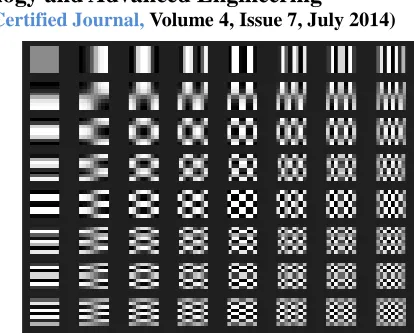
[image:4.612.335.542.115.282.2]

For x, y = 0, 1, 2… N −1. The 2-D functioning can be produced by multiplying the horizontally oriented 1-D with vertically oriented set of the same functions.[11]

Figure 2. Two dimensional DCT basis functions (N = 8). Neutral gray represents zero, white represents positive amplitudes, and black

represents negative amplitude.

E.Discrete Wavelet Transform (DWT)

The fundamental concept of DWT for one-dimensional signals is briefly explained as fallows. A signal is break down into two fragments, generally the low frequency part and the high frequency. This break down is named as decomposition. The edge aspects of the signal are generally enclosed to the high frequencies part.

The signal is handed down through a number of high pass filters to evaluate the high frequencies, and then passed through a number of low pass filters to evaluate the low frequencies. Filters with cut-off frequencies are utilized to examine the signal at different resolutions. Let's guess that x[n] is the initial signal, having a frequency band of 0 to π rad/s. The signal x[n] is initially passed through a half band high pass filter g[n] and a low pass filter h[n]. Following the filtering, half of the trials can be eradicated based on the Nyquist’s rule, as the signal now has the top frequency of π/2 radians rather than of π. The signal can consequently be subsampled by 2, merely by neglect every second sample. This comprises one level of decomposition and can arithmetically be stated as follows:

𝑦ℎ𝑖𝑔ℎ,𝑘- = ∑ 𝑥,𝑘-𝑔,2𝑘 −

𝑛-𝑛

𝑦𝑙𝑜𝑤,𝑘- = ∑ 𝑥,𝑘-𝑕,2𝑘 −

𝑛-𝑛

(19)

(5)

International Journal of Emerging Technology and Advanced Engineering

706

The yields of the high pass and low pass filters are named as DWT coefficients. The original image can be reconstructed utilizing this DWT. The reconstructed method is known as the Inverse Discrete Wavelet Transform (IDWT).

The signals at every level are passed through the synthesis filters g’ [n], and h’ [n], and then added. The synthesis and analysis filters are alike to each other, except for a time reversal. So, the reconstruction formula becomes (for each layer)

𝑥,𝑛- = ∑ 𝑦ℎ𝑖𝑔ℎ,𝑘-𝑔,2𝑘 − 𝑛- + 𝑦𝑙𝑜𝑤,𝑘-𝑕,2𝑘 − 𝑛-𝑛

(20)

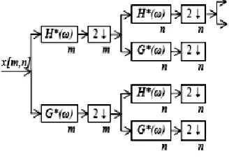
The DWT and IDWT for a one-dimensional signal can be also described in the form of two channel tree structured filter banks. The DWT and IDWT for a two-dimensional image x [m, n] can be similarly defined by implementing DWT and IDWT for each dimension m and n separately

[image:5.612.325.566.133.302.2]

𝐷𝑊𝑇𝑛,𝐷𝑊𝑇𝑚,𝑥,𝑚, 𝑛--, which is shown in Figure 1.

Fig.3: DWT for two-dimensional images

[image:5.612.329.555.374.489.2]

An image can be decomposed into a pyramidal structure, which is shown in Figure 4, with various band information: low-low frequency band LL, low-high frequency band LH, high-low frequency band HL, high frequency band HH.

Fig.4: Pyramidal structure

II. SIMULATION RESULTS

Figure 4: GUI figure window in Matlab

This is Graphical User Interface (GUI) window created in Matlab which is used in this work for simulation of all techniques.

Simulation Results for DWT, FFT and DCT :

(a) (b)

[image:5.612.83.247.380.493.2]

Figure:-5.(a)Gray converted Image (b) Reconstructed Image after processing with DWT

Figure 6: curve of Gaussian noise BER for DWT source coding with OFDM

-2 0 2 4 6 8 10

10-5 10-4 10-3 10-2 10-1

Eb/No, dB

B

it

E

rr

o

r

R

a

te

Gaussian Noise BER curve for Wavelet source coding with OFDM

[image:5.612.335.545.513.699.2] [image:5.612.100.240.574.683.2]

(6)

International Journal of Emerging Technology and Advanced Engineering

[image:6.612.338.546.141.315.2]

707

Figure 7: PSNR curve for DWT source coding with OFDM

(a) (b)

[image:6.612.69.266.143.317.2]

Figure:-8.(a)Gray converted Image (b) Reconstructed Image after processing with FFT

[image:6.612.333.554.330.451.2]

Figure:-9Gaussian Noise BER curve for Fast Fourier transform with OFDM

Figure:-10 PSNR curve for Fast Fourier transform with OFDM

(a) (b)

Figure:-11.(a)Gray converted Image (b) Reconstructed Image after processing with DCT

Figure:-3Gaussian Noise BER curve for DCT with OFDM

-4 -2 0 2 4 6 8 10

26 28 30 32 34 36 38 40 42 44 46

Eb/No, dB

P

S

N

R

PSNR

-2 0 2 4 6 8 10

10-5

10-4

10-3

10-2

10-1

Eb/No, dB

B

it

E

rr

o

r

R

a

te

Gaussian Noise BER curve for fft source coding with OFDM

theory simulation

-4 -2 0 2 4 6 8 10

10 15 20 25 30 35 40 45 50 55 60

Eb/No, dB

P

S

N

R

PSNR

-2 0 2 4 6 8 10

10-5

10-4

10-3

10-2

10-1

Eb/No, dB

B

it

E

rr

o

r

R

a

te

Gaussian Noise BER curve for DCT source coding with OFDM

[image:6.612.56.284.347.464.2] [image:6.612.335.544.469.638.2] [image:6.612.60.277.487.665.2]

(7)

International Journal of Emerging Technology and Advanced Engineering

[image:7.612.65.271.139.309.2]

708

Figure:-4 PSNR curve for Discrete Cosine transform with OFDM

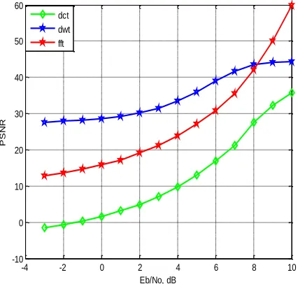
Figure:-4 Comparative graph for PSNR of DCT, DWT and FFT with OFDM

Variation between Signal to Noise Ratio (SNR)(Eb N0⁄ , dB) and Peak Signal to Noise Ratio was shown in figure. The above figure shows the comparisons of PSNR curve of DWT, DCT and FFT , where PSNR values increases according to Eb N0⁄ .

[image:7.612.305.584.165.332.2]

Also we compare all techniques on the basis of other simulation parameters like WPSNR, MSE, SSIM CORR2.

Table 1

Values of different parameters for Different Methods

The above table shows the comparative analysis of DCT, DWT, FFT, RS Code and LDPC.

III. CONCLUSION

OFDM is a very attractive technique for multicarrier transmission and has become one of the standard choices for high speed data transmission over a communication channel. It has various advantages; but also has one major drawback: it has a very high PAPR.

The above result shows the comparisons of PSNR curve of DWT, DCT and FFT, where PSNR values increases according to Eb N0⁄ . At very low Eb N0⁄ i.e is −4 dB the PSNR value of DWT is 28 dB approximately.

Maximum at Eb N0⁄ is 10 dB , PSNR is 46 dB approx for DWT. The above result shows that even low Eb N0⁄ the value of PSNR in DWT maintains its appreciable range.

Higher value of PSNR indicates better results. The result shows that if SNR value is low than DWT is much better from all existing methods. But if SNR value increases than FFT is better than all other methods.

REFERENCES

[1] R.W. Chang, “Synthesis of band-limited orthogonal signals for

multichannel data transmission”, Bell System tech. 1966.

[2] B.R. Saltzberg, “Performance of an efficient parallel data

transmission system”,IEEE trans. Comm., 1967.

[3] S.B.Weinstein and P.M. Ebert, “Data transmission by

frequency-Division multiplexing using the discrete Fourier transform”, IEEE, 1971.

-4 -2 0 2 4 6 8 10

-5 0 5 10 15 20 25 30 35 40

Eb/No, dB

P

S

N

R

PSNR

-4 -2 0 2 4 6 8 10

-10 0 10 20 30 40 50 60

Eb/No, dB

P

S

N

R

dct dwt fft

Parameters

Name of Different Method used

DCT DWT FFT RS

Code LDPC

PSNR 43.3242 46.1062 56.9025 24.8553 27.7056

WPSNR 54.189 56.2711 68.4768 29.9683 33.5803

MSE 3.0246 1.5939 0.13269 212.5957 110.287

SSIM 0.9886 0.98847 0.99901 0.58706 0.68585

[image:7.612.62.275.344.547.2]

(8)

International Journal of Emerging Technology and Advanced Engineering

709

[4] A. Peled and A. Ruiz, “frequency domain data transmission using

reduced computational complexity algorithms”, in proc. IEEE, 1980.

[5] Radio broadcasting systems; digital audio broadcasting (DBA) to

mobile portable and fixed receivers, European Telecommunications Standards Institute Valbonne, France 1995.

[6] T.KELLER et al. Report on digital audio radio laboratory tests.

Technical report, Electronic Industries Association May 1995.

[7] R. G. Gallager, “Low density parity check codes”, IRE Transaction

Information Theory IT -8, 21, 1962.

[8] H. Futaki, and T. Ohtsuki, “Low-Density Parity-Check (LDPC)

Coded OFDM systems”, IEEE, 2001.

[9] I.M.Arijon and P.G.Farrall, “Performance of an OFDM system in

frequency selective channels using Reed-Solomon coding Schemes”, IEEE, 1996.

[10] Q.Zhang, W. Zhu, Zu Ji, and Y. Zhang, “A Power-Optimized Joint

Source Channel Coding for Scalable Video Streaming over Wireless Channel," IEEE ISCAS’01, May, 2001, Sydney, Australia.

[11] W. B. Pennebaker and J. L. Mitchell, “JPEG – Still Image Data