comm
en
t
re
v
ie
w
s
re
ports
de
p
o
si
te
d r
e
sea
rch
refer
e
e
d
re
sear
ch
interacti
o
ns
inf
ormation
Statistical methods for ranking differentially expressed genes
Per Broberg
Address: Molecular Sciences, AstraZeneca Research and Development Lund, S-221 87 Lund, Sweden.
Correspondence: Per Broberg. E-mail: [email protected].
© 2003 Broberg; licensee BioMed Central Ltd. This is an Open Access article: verbatim copying and redistribution of this article are permitted in all media for any purpose, provided this notice is preserved along with the article's original URL.
Statistical methods for ranking differentially expressed genes
In the analysis of microarray data the identification of differential expression is paramount. Here I outline a method for finding an optimal test statistic with which to rank genes with respect to differential expression. Tests of the method show that it allows generation of top gene lists that give few false positives and few false negatives. Estimation of the false-negative as well as the false-positive rate lies at the heart of the method.
Abstract
In the analysis of microarray data the identification of differential expression is paramount. Here I outline a method for finding an optimal test statistic with which to rank genes with respect to differential expression. Tests of the method show that it allows generation of top gene lists that give few false positives and few false negatives. Estimation of the negative as well as the false-positive rate lies at the heart of the method.
Background
Microarray technology has revolutionized modern biological research by permitting the simultaneous study of genes com-prising a large part of the genome. The blessings stemming from this are accompanied by the curse of high dimensional-ity of the data output. The main objective of this article is to explore one method for ranking genes in order of likelihood of being differentially expressed. Top gene lists, that give few false positives and few false negatives, are the output. As the interest is mainly in ranking for the purpose of generating top gene lists, issues such as calculation of p-values and correc-tion for multiple tests are of secondary importance.
Microarrays have an important role in finding novel drug tar-gets; the thinking that guides the design and interpretation of such experiments has been expressed by Lonnstedt and Speed [1]: "The number of genes selected would depend on the size, aim, background and follow-up plans of the experi-ment." Often, interest is restricted to so-called 'druggable' target classes, thus thinning out the set of eligible genes con-siderably. It is generally sensible to focus attention first on druggable targets with smaller p-values (where the p-value is the probability of obtaining at least the same degree of differ-ential expression by pure chance) before proceeding to ones with larger p-values. In general, p-values have the greatest
impact on decisions regarding target selection by providing a preliminary ranking of the genes. This is not to say that mul-tiplicity should never be taken into account, or that the meth-od presented here replaces correction for multiplicity. On the contrary, the approach provides a basis for such calculations (see Additional data files).
The approach presented here could be applied to different types of test statistics, but one particular type of recently pro-posed statistic will be used. In Tusher [2] a methodology based on a modified t-statistic is described:
where diff is an effect estimate, for example, a group mean difference, S is a standard error, and S0 is a regularizing con-stant. This formulation is quite general and includes, for ex-ample, the estimation of a contrast in an ANOVA. Setting S0 = 0 will yield a t-statistic. The constant, called the fudge con-stant, is found by removing the trend in d as a function of S in moving windows across the data. The technical details are outlined in [3]. The statistic calculated in this way will be re-ferred to as SAM. The basic idea with d is to eliminate some false positives with low values of S, see Figure 1.
Published: 29 May 2003 Genome Biology 2003, 4:R41
Received: 9 December 2002 Revised: 25 March 2003 Accepted: 7 May 2003 The electronic version of this article is the complete one and can be
found online at http://genomebiology.com/2003/4/6/R41
A previous version of this manuscript was made available before peer review at http://genomebiology.com/2002/3/9/preprint/0007
d diff
S S
=
+
( )
0
It is more relevant to optimize with respect to false-positive and false-negative rates. This is the basic idea behind the new approach. The idea is to jointly minimize the number of genes that are falsely declared positive and the number of genes falsely declared negative by optimizing over a range of values of the significance level a and the fudge constant S0. How well this is achieved can be judged by a receiver operating charac-teristics (ROC) curve, which displays the number of false pos-itives against the number of false negatives expressed as proportions of the total number of genes.
An alternative to the statistic (1) is d = diff/√(S02 + S2), or d = diff/√(wS02 + (1 - w)S2) for some weight w, which is basically the statistic proposed in Baldi [4]. Its performance appears to be very similar to that of (1) (data not shown). A software im-plementation in R code within the package SAG [5,6] is avail-able from [7] via the function samroc.
Results
The criterionA comparison of methods in terms of their ROC curves is pre-sented in Lonnstedt [1]. A method whose ROC curve lies be-low another one (has smaller ordinate for given abscissa) is preferred (Figure 2). A method which has a better ROC curve, in this sense, will produce top lists with more differentially
expressed genes (DEGs), fewer non-DEGs, and, consequent-ly, will leave out fewer DEGs. Furthermore, such a method will give higher average ranks to the DEGs, if the ranking is such that high rank means more evidence of differential ex-pression. Superiority in terms of average ranks is a weaker as-sertion than superiority in terms of ROC curves (see Additional data files for a proof). If it is desirable to compare methods with respect to their ROC curves, then the estima-tion procedures should find parameter estimates that opti-mize the ROC curve. This section suggests a goodness criterion based on the ROC curve.
False discovery rate (FDR) may be defined as the proportion of false positives among the significant genes, see [2]. False-positive rate (FP) may be defined as the number of false pos-itives among the significant genes divided by the total number of genes. Similarly, we define the false-negative rate (FN) as the number of false negatives among the nonsignificant genes divided by the total number of genes, the true-positive rate (TP) as the number of true positives divided by the total number of genes, and, the true-negative rate (TN) as the number of true negatives divided by the total number of genes.
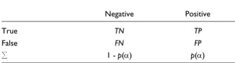
[image:2.612.56.301.85.322.2]In Table 1 relations involving these entities are displayed. For instance, the proportion of unchanged genes (non-DEGs), p0, equals the sum of the proportion of true negative and the Figure 1
The effect of S0. With real microarray data the absolute value of the t -statistic often shows erratic behavior for small values of the standard error S, with an increased risk of false positives. By choosing the constant S0 in equation (1) wisely one can alleviate this problem. In the right panel we see that the statistic d in equation (1) downplays the importance of some of the genes with low standard error, compared to the t-statistic (left panel). Data from Golub [16] were used, and S0 was chosen as the 5% percentile of S values (see also Discussion).
0 5 10 15 20 25 30 S
|
[image:2.612.315.555.85.308.2]t
-statistic|
0 5 10 15 20 25 30 S
|
d
-statistic|
0 2 4 6 8 10
0 2 4 6 8 10
Figure 2
ROC curve. This graph displays the number of false negatives (differentially expressed genes (DEGs) not included) versus the number of false positives (non-DEGs included) found on top lists of increasing sizes, expressed as proportions of the total number of genes. The distance C gives an optimal value of equation (2). A method whose ROC curve lies below that of another method is preferable, as it will give more DEGs and fewer non-DEGs on any top list of any size, as explained in Additional data. Hence method 1 is preferable to method 2.
0.0 0.2 0.4 0.6 0.8 1.0
False negative
F
alse positiv
e
C
Method 1 Method 2
comm
en
t
re
v
ie
w
s
re
ports
refer
e
e
d
re
sear
ch
de
p
o
si
te
d r
e
se
a
rch
interacti
o
ns
inf
o
rmation
proportion of false positive: p0 = TN + FP, and the proportion of significant genes at a certain significance level α equals the sum of the true positives and the false positives: p(α) = TP + FP. It is intuitive that the criterion to be minimized should be an increasing function of FP and FN. Any top list produced should have many DEGs and few non-DEGs.
Assume that we can, for every combination of values of the significance level α and the fudge constant S0, calculate (FP, FN). The goodness criterion is then formulated in terms of the distance of the points (FP, FN) to the origin (which point cor-responds to no false positives and no false negatives, see Fig-ure 2), which in mathematical symbols may be put as
The optimal value of (α, S0) will be the one that minimizes (2). It is for practical reasons not possible to do this minimization over every combination, so the suggestion is to estimate the criterion over a lattice of (α, S0) values and pick the best combination.
If one has an assessment regarding the relative importance of FP and FN, that may be reflected in a version of the criterion (2) that incorporates a weight λ that reflects the relative im-portance of FP compared to FN: Cλ = √(λ2 FP2 + FN2). The
choice λ = (1 - p0)/p0 corresponds to another type of ROC curve, which displays the proportion of true (TP/(1 - p0)) against the proportion of false (FP/p0) (see Additional data files). Other goodness criteria are possible, such as the sum of FP and FN or the area under the curve in Figure 2. For more details and other approaches see, for example [8,9].
Calculating p-values
Using the permutation method to simulate the null distribu-tion (no change) we can obtain a p-value for a two-sided test, as detailed below. Loosely speaking, in each loop of the simu-lation algorithm the group labels are randomly rearranged, so that random groups are formed, the test statistic is calculated for this arrangement and the value is compared to the ob-served one. How extreme the obob-served test statistic is will be
judged by counting the number of times that more extreme values are obtained from the null distribution.
The data matrix X has genes in rows and arrays in columns. Consider the vector of group labels fixed. The permutation method consists of repeatedly permuting the columns (equiv-alent to rearranging group labels), thus obtaining the matrix
X*, and calculating the test statistic for each gene and each permutation. Let d(j)*k be the value of the statistic of the jth
gene in the kth permutation of columns. Then the p-value for gene i equals
where M is the number of genes, d(i) the observed statistic for gene i, B the number of permutations and '#' denotes the car-dinality of the set [2,10,11]. In words, this gives the relative frequency of randomly generated test statistics with an abso-lute value that exceeds the observed value of gene i. The for-mula (3) combines the permutation method in [2] and the p -value calculation in [10]. These p-values are such that a more extreme value of the test statistic will yield a lower p-value.
Given the significance level α (p-values less than α are consid-ered significant), the proportion of the genes considconsid-ered dif-ferentially expressed is
which is the relative frequency of genes with a p-value less than α.
The current version of samroc uses the estimate
where qX is the X% percentile of the d* (compare [3]). This es-timate makes use of the fact that the genes whose test statis-tics fall in the quartile range will be predominantly the unchanged ones. More material on this matter is in the Addi-tional data files.
Estimating FP
Going via results for the FDR in Storey [12] (see also [13,14]) it is possible to derive the estimate
[image:3.612.53.294.129.194.2]which is the proportion of unchanged genes multiplied by the probability that such a gene produces a significant result. For a derivation see the Additional data files.
Table 1
The unknown distribution of true and false positives and negatives
Negative Positive
True TN TP
False FN FP
冱 1 - p(α) p(α)
The proportion of incorrectly called genes equals FN + FP, and the proportion called significant equals p(α) = TP + FP.
C= FP2+FN2
( )
2P
d j d j d i
B M
i
k k
=
{
( )
( )
≥( )
}
×
( )
# *: *
3
p i P
M
i
a a
( )
=# :{
≤}
,( )
4ù # : /
p i q d i q
M
0= 25 2 75 5
≤
( )
≤{
}
( )
ù ù
Estimating FN
From Table 1 one obtains, as outlined in the Additional data files,
FN = 1 - p0(1 - α) - p(α) (6)
To get an intuitive feel for this equality, just note that the sec-ond term is the proportion unchanged multiplied by the prob-ability of such genes not being significant, which estimates TN, and that the third term corresponds to the positive (TP + FP). Subtracting the proportion of these two categories from the whole will leave us with the FN.
Estimating the criterion
The entities we need for the optimisation are given by the estimates
and
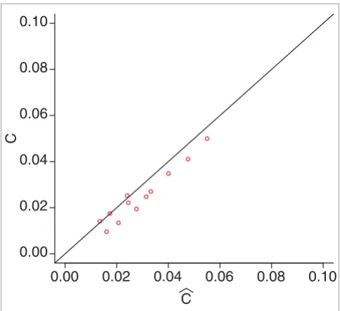
A scatter plot of the estimate of the criterion
versus the true value is shown in Figure 3, and reveals a good level of accuracy.
Tests
A detailed account of the results is given in the Additional data files, where datasets, data preprocessing, analysis and results are described in enough detail to enable the results to be reproduced.
When testing methods in this field it is difficult to find suita-ble data for which something is known about the true status of the genes. If one chooses to simulate, then the distributions may not be entirely representative of a real-life situation. If one can find non-proprietary real-life data, then the knowl-edge as to which genes are truly changed may be uncertain. To provide adequate evidence of good performance it is neces-sary to provide such evidence under different and reproduci-ble conditions.
In the comparison, samroc, t-test, Wilcoxon, the Bayesian method in [1], and SAM [2] were competing. By the t-test I mean the unequal variance t-test: t = (mean1 - mean2)/√(s12/
n1 + s22/n
2) for sample means mean1 and mean2 and sample variances s12, s
22. The Wilcoxon rank sum test is based on the sum Ws of the ranks of the observations in one of the groups Ws = R1...+ Rn1 [15]. The Bayesian method calculates the pos-terior odds for genes being changed (available as functions
stat.bay.est.lin in the R package SAG, and stat.bayesian in
the R package sma [1,5]). The method starts from the as-sumption of a joint a priori distribution of the effect estimate and the standard error. The former is assumed normal and the latter inverse Gamma.
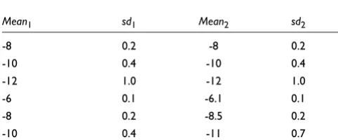
Simulated cDNA data
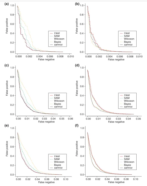
The normal distributions modeled after real-life cDNA data used in Baldi and Long [4] were used here to provide a testing ground for the methods (Table 2). In each simulation two groups of four arrays each were created. Three datasets with 1%, 5% and 10% DEGs were generated using the normal dis-tributions. In all cases samroc and the t-test coincided (S0 = 0), and were the best methods in terms of the ROC curves. Theory predicts that the t-test is optimal in this situation (see Additional data files). When data were antilogarithm-trans-formed, giving rise to lognormal distributions, samroc again came out best, followed by the Bayes method. The t-test falls behind this time. Figure 4 gives a graphical presentation of the results in terms of ROC curves.
Oligonucleotide leukemia data
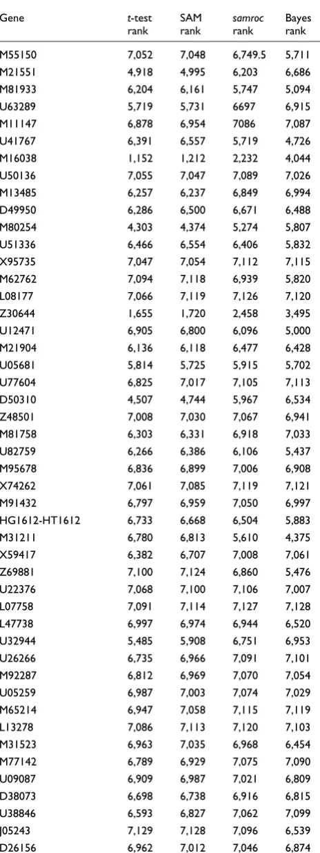
[image:4.612.57.299.85.307.2]The data on two types of leukemia, ALL and AML, appeared in Golub et al. [16,17]. Samples of both types were hybridized to 38 arrays. In [17], 50 genes were identified as DEGs using statistical analysis of data from the full set of arrays. For these data it is impossible to calculate a ROC curve as the DEGs are unknown. Instead, performance was assessed in terms of the average rank of the 50 genes, after all genes were ranked by their likelihood of being DEGs according to each of the meth-ods. Using just three arrays from each of the two groups, sam-roc gave the best results, followed by SAM (Table 3). This Figure 3
Estimates of the criterion. The true and the estimated value of the goodness criterion √(FP2 + FN2). Using data from the simulated cDNA distributions, the true FP and FN were calculated and then estimated. Finally, the goodness criterion was calculated and displayed in a scatter plot, showing a good correspondence between estimate and estimand.
0.00
0.02
0.04
0.06
0.08
0.10
C
C
0.00
0.02
0.04
0.06
0.08
0.10
ù ù
FN = −1 p0
(
1−a)
−p( )
aù ù
FP=p0a
ˆ
ˆ
comm
en
t
re
v
ie
w
s
re
ports
refer
e
e
d
re
sear
ch
de
p
o
si
te
d r
e
se
a
rch
interacti
o
ns
inf
o
[image:5.612.57.552.84.710.2]rmation
Figure 4 (see legend on next page)
0.00 0.02 0.04 0.06 0.08 0.10 False negative
F
alse positiv
e
0.00 0.02 0.04 0.06 0.08 0.10 False negative
F
alse positiv
e
0.00 0.01 0.02 0.03 0.04 0.05 False negative
F
alse positiv
e
0.00 0.01 0.02 0.03 0.04 0.05 0.06 False negative
F
alse positiv
e
0.000 0.002 0.004 0.006 0.008 0.010 False negative
F
alse positiv
e
0.000 0.002 0.004 0.006 0.008 0.010 False negative
F
alse positiv
e
t-test SAM Wilcoxon Bayes samroc
0.0 0.2 0.4 0.6 0.8 1.0
0.0 0.2 0.4 0.6 0.8 1.0
0.0 0.2 0.4 0.6 0.8 1.0
0.0 0.2 0.4 0.6 0.8 1.0 0.0 0.2 0.4 0.6 0.8 1.0 0.0 0.2 0.4 0.6 0.8 1.0
SAM Wilcoxon Bayes t-test
samroc
t-test SAM Wilcoxon Bayes samroc
SAM Wilcoxon Bayes t-test
samroc
t-test SAM Wilcoxon Bayes samroc
SAM Wilcoxon Bayes t-test
samroc
(a)
(b)
(c)
(d)
means that a necessary but not sufficient condition for the su-periority of samroc in terms of ROC curves is satisfied (see Additional data files).
Affymetrix spiking experiment data
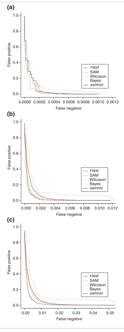
In this test, data generated by Affymetrix in an experiment where 14 transcripts were spiked at known quantities (Table 4) [18,19] were used. Using three arrays from each of two groups of arrays where 14 probe sets (genes) differ, further datasets with 140 and 714 DEGs were generated by a boot-strap procedure. Thus there were three datasets with roughly 0.1%, 1% and 5% DEGs. In two of these three settings samroc performed best, and in one case (0.1%) SAM and the Bayes method were better. Figure 5 gives a graphical presentation of these results in terms of ROC curves.
Discussion
Whether to look at data on a log scale or not is a tricky ques-tion, and is beyond the scope of this article. However, the best performance by the tests considered was achieved when data were lognormal (see Additional data files). Normal, lognor-mal and real-life data were all included in order to supply a varied testing ground.
As pointed out in [20], the Bayes statistic is for ranking pur-poses equivalent to a penalized t-statistic tp = (mean1
-mean2)/√(a1 + S2). Here a
1 is a scale parameter related to the
a priori distribution of the standard error. This means that it
is, at least in form, closely related to the t-test, SAM and sam-roc. SAM, on the other hand, chooses as its fudge constant the value among the percentiles of S, which minimizes the coeffi-cient of variation of the median absolute deviation of the test statistic computed over a number of percentiles of S [3]. It is interesting to note how different the three related statistics the Bayes method, SAM and samroc turn out in practice.
One clue to why this difference occurs emerges when compar-ing the denominators of SAM/samroc and Bayes more close-ly. First square the denominators of (1) and the representation of Bayes above. We obtain (a + S)2 = a2 + 2aS + S2 for (1) and a
1 + S2 for Bayes (where generally a1≥ a2). For large values of S the former will exceed the latter. This means that SAM/samroc will downplay the importance of the results for high expressing genes in a way that the Bayes method does not.
But there is also another difference. The Bayes method seems to achieve best when the number of false positives is allowed to grow rather large. The constant a corresponds to a large percentile in the distribution of the S2 values (see Additional data files). Whereas the constant in SAM will generally be rather small, often the 5-10% percentile of the S values, the constant in the Bayes method will correspond to at least the 40% percentile of the S2 values. It seems that using a large percentile will give a good performance when the number of false positives grows large. This observation is consistent with the observation made in Lonnstedt and Speed [1] that the par-ticular version of SAM, which always uses the 90% percentile, will pass the Bayes method when the number of false posi-tives is allowed to grow large. Also, samroc will in general make use of a smaller percentile, albeit that samroc shows greater spread between datasets in the values chosen, as a re-sult of its adaptation to the features specific to the data at hand.
Samroc is the only method that makes explicit use of the number of changed genes in the ranking. If one has reason to believe, for example from studying expression (3), that there are very few DEGs (<< 1%), then samroc is probably not the first choice. Probably SAM or the Bayes method is more Figure 4 (see previous page)
[image:6.612.56.297.611.711.2]Simulated normal and log-normal data. (a) Normal distribution, 1% DEGs. As expected with independent normally distributed observations, the t-test will perform quite well, and is matched by samroc, which in this case equals the equal-variance t-test. The Bayes method has problems with these data, with SAM and Wilcoxon somewhere in between these extremes. (b) Lognormal distribution, 1% DEGs. samroc may have a slight advantage for shorter lists, whereas the Bayes method is better for longer lists, where the number of false positives is larger. The other three methods lag behind, but not by much. (c) Normal distribution, 5% DEGs. The t-test and samroc coincide; samroc is now equivalent to the equal-variance t-test, which behaves in the same way as the unequal-variance t-test in this case. (d) Lognormal distribution, 5% DEGs. The difference between methods is less when data are exponentiated. However, samroc has the edge for a wide range of cutoffs, but the Bayes method catches up when more genes are selected. The other three methods are struggling to avoid last spot. (e) Normal distribution, 10% DEGs. Again the samroc and the t-test coincide and the Bayes method has problems with normal data. SAM is also lagging behind, while the other three are very close together. (f) Lognormal distribution, 10% DEGs. samroc comes out well; Wilcoxon has the worst performance, SAM and the t-test are scarcely better, while the Bayes method is intermediate.
Table 2
The normal distributions simulated defined by their means and standard deviations
Mean1 sd1 Mean2 sd2
-8 0.2 -8 0.2
-10 0.4 -10 0.4
-12 1.0 -12 1.0
-6 0.1 -6.1 0.1
-8 0.2 -8.5 0.2
-10 0.4 -11 0.7
comm
en
t
re
v
ie
w
s
re
ports
refer
e
e
d
re
sear
ch
de
p
o
si
te
d r
e
se
a
rch
interacti
o
ns
inf
o
rmation
useful in these situations. If, on the other hand, the number of DEGs is reasonably large, samroc is conjectured to take prec-edence over SAM, and to be more robust than the Bayes method. Furthermore, one can argue that the kind of experi-ments undertaken in drug discovery would more often than not end in comparisons in which the biological systems show vast differences in a large number of genes, mostly as a down-stream effect of some shock to the system.
The proposed method comes out better than or as good as the original SAM statistic in most tests performed. The samroc statistic is robust and flexible in that it can address all sorts of problems that suit a linear model. The methodology adjusts the fudge constant flexibly and achieves an improved per-formance. The algorithm gives fewer false positives and fewer false negatives in many situations, and was never much worse than the best test statistic in any circumstance. However, a typical run with real-life data will take several hours on a desktop computer. To make this methodology better suited for production it would be a good investment to translate part of the R code, or the whole of it, into C.
To improve on standard univariate tests one must make use of the fact that data are available on a large number of related tests. One way of achieving this goal has been shown in this paper. The conclusion is that it is possible and sensible to cal-ibrate the test with respect to estimates of the false-positive and false-negative rates.
Additional data files
[image:7.612.56.292.84.718.2]A zip file (Additional data file 1) containing the R package SAG for retrieval, preparation and analysis of data from the Affymetrix GeneChip and the R script (Additional data file 2) are available with the online version of this article. An appen-dix (Additional data file 3) giving further details of the statis-tical methods and the samroc algorithm is also available as a PDF file.
Figure 5
0.00 0.01 0.02 0.03 0.04 0.05 False negative
F
alse positiv
e
0.000 0.002 0.004 0.006 0.008 0.010 0.012 False negative
F
alse positiv
e
0.0000 0.0002 0.0004 0.0006 0.0008 0.0010 0.0012 False negative
F
alse positiv
e
t-test SAM Wilcoxon Bayes samroc
0.0 0.2 0.4 0.6 0.8 1.0
0.0 0.2 0.4 0.6 0.8 1.0
0.0 0.2 0.4 0.6 0.8 1.0
t-test SAM Wilcoxon Bayes samroc
t-test SAM Wilcoxon Bayes samroc
(a)
(b)
(c)
Figure 5
Acknowledgements
Ingrid Lonnstedt generously made the code to a linear models version of stat.bay.est available. Comments from Terry Speed are gratefully acknowl-edged, among them the suggestion to use spike data and ROC curves in the evaluation, as is the input from Brian Middleton and Witte Koopmann.
References
1. Lonnstedt I, Speed TP: Replicated microarray data.Stat Sinica 2002, 12:31-46.
2. Tusher VG, Tibshirani R, Chu G: Significance analysis of micro-arrays applied to the ionizing radiation response.Proc Natl Acad Sci USA 2001, 98:5116-5121.
[image:8.612.58.290.121.739.2]3. Chu G, Narasimhan B, Tibshirani R, Tusher VG: SAM Version 1.12: Table 3
Ranking based on the leukemia data [16]
Gene t-test
rank
SAM rank
samroc
rank
Bayes rank
M55150 7,052 7,048 6,749.5 5,711
M21551 4,918 4,995 6,203 6,686
M81933 6,204 6,161 5,747 5,094
U63289 5,719 5,731 6697 6,915
M11147 6,878 6,954 7086 7,087
U41767 6,391 6,557 5,719 4,726
M16038 1,152 1,212 2,232 4,044
U50136 7,055 7,047 7,089 7,026
M13485 6,257 6,237 6,849 6,994
D49950 6,286 6,500 6,671 6,488
M80254 4,303 4,374 5,274 5,807
U51336 6,466 6,554 6,406 5,832
X95735 7,047 7,054 7,112 7,115
M62762 7,094 7,118 6,939 5,820
L08177 7,066 7,119 7,126 7,120
Z30644 1,655 1,720 2,458 3,495
U12471 6,905 6,800 6,096 5,000
M21904 6,136 6,118 6,477 6,428
U05681 5,814 5,725 5,915 5,702
U77604 6,825 7,017 7,105 7,113
D50310 4,507 4,744 5,967 6,534
Z48501 7,008 7,030 7,067 6,941
M81758 6,303 6,331 6,918 7,033
U82759 6,266 6,386 6,106 5,437
M95678 6,836 6,899 7,006 6,908
X74262 7,061 7,085 7,119 7,121
M91432 6,797 6,959 7,050 6,997
HG1612-HT1612 6,733 6,668 6,504 5,883
M31211 6,780 6,813 5,610 4,375
X59417 6,382 6,707 7,008 7,061
Z69881 7,100 7,124 6,860 5,476
U22376 7,068 7,100 7,106 7,007
L07758 7,091 7,114 7,127 7,128
L47738 6,997 6,974 6,944 6,520
U32944 5,485 5,908 6,751 6,953
U26266 6,735 6,966 7,091 7,101
M92287 6,812 6,969 7,070 7,054
U05259 6,987 7,003 7,074 7,029
M65214 6,947 7,058 7,115 7,119
L13278 7,086 7,113 7,120 7,103
M31523 6,963 7,035 6,968 6,454
M77142 6,789 6,929 7,075 7,090
U09087 6,909 6,987 7,021 6,809
D38073 6,698 6,738 6,916 6,815
U38846 6,593 6,827 7,062 7,099
J05243 7,129 7,128 7,096 6,539
D26156 6,962 7,012 7,046 6,874
X15414 6,608 6,790 6,117 5,023
S50223 6809 6,861 6,629 5,886
X74801 6,726 6,895 7,032 6,996
Average 6,367.8 6,443.88 6,550.51 6,371.36
[image:8.612.316.556.279.500.2]Results for the leukemia data using only the first four samples from ALL and AML. The higher the average rank the better the method has been at identifying the probe sets that are changed.
Table 4
Affymetrix spike experiment
Transcript Experiments
M, N, O, P Q, R, S, T
1 512 1,024
2 1,024 0
3 0 0.25
4 0.25 0.5
5 0.5 1
6 1 2
7 2 4
8 4 8
9 8 16
10 16 32
11 32 64
12 512 1024
13 128 256
14 256 512
The table shows the part of the design of the Affymetrix spike experiment used as a testing ground for methods of ranking genes with respect to differential expression. Out of the 12,626 probe sets on the U95A array 14 transcripts have been spiked at known quantities in picomols selected according to a Latin square design. Here 'experiment' (M, N, O..., T) refers to a set of three arrays with the same spiking. The numbers indicate the amount of spike transcript in pM.
Table 3 (Continued)
comm
en
t
re
v
ie
w
s
re
ports
refer
e
e
d
re
sear
ch
de
p
o
si
te
d r
e
se
a
rch
interacti
o
ns
inf
o
rmation
user's guide and technical document. [http://www-stat.stanford.edu/~tibs/SAM/].
4. Baldi P, Long AD: A Bayesian framework for the analysis of microarray expression data: regularized t-test and statistical inferences of gene changes.Bioinformatics 2001, 17:509-519. 5. The Comprehensive R Archive Network
[http://www.cran.r-project.org]
6. Ihaka R, Gentleman R: R: a language for data analysis and graphics.J Comput Graph Stat 1996, 5:299-314.
7. Supplementary files: SAG and simulation script [http:// home.swipnet.se/pibroberg]
8. Lovell DR, Dance CR, Niranjan M, Prager RW, Dalton KJ: Ranking the effect of different features on the classification of dis-crete valued data. In Engineering Applications of Neural Networks. Kingston on Thames, London; 1996:487-494.
9. Genovese C, Wasserman L: Operating characteristics of the FDR procedure. Technical Report. New York, Carnegie Mellon University 2001.
10. Dudoit S, Yang YH, Speed TP, Callow MJ: Statistical methods for identifying differentially expressed genes in replicated cDNA microarray experiments.Stat Sinica 2002, 12:111-140.
11. Davison AC, Hinkley DV: Bootstrap Methods and their Application. Cambridge, UK: Cambridge University Press; 1997.
12. Storey JD: A direct approach to false discovery rates. Technical Report. Stanford, CA: Stanford University; 2001.
13. Efron B, Tibshirani R, Storey JD, Tusher VG: Empirical Bayes anal-ysis of a microarray experiment.J Am Stat Assoc 2001, 96: 1151-1160.
14. Benjamini Y, Hochberg Y: Controlling the false discovery rate: a practical and powerful approach to multiple testing.J R Stat Soc B 1995, 57:963-971.
15. Lehmann EL: Nonparametrics: Statistical Methods Based on Ranks. San Francisco, CA: Holden-Day; 1975.
16. Golub TR, Slonim DK, Tamayo P, Huard C, Gaasenbeek M, Mesirov JP, Coller H, Loh ML, Downing JR, Caligiuri MA, et al.: Molecular classification of cancer: class discovery and class prediction by gene expression monitoring.Science 1999, 286:531-537. 17. Whitehead Institute Center for Genome Research: Cancer
Genomics Publications Data Sets
[http://www-genome.wi.mit.edu/cgi-bin/cancer/datasets.cgi] 18. Speed Group Microarray Page - Affymetrix data analysis
[http://www.stat.berkeley.edu/users/terry/zarray/Affy] 19. Affymetrix [http://www.affymetrix.com]
20. Smyth GK, Yang YH, Speed TP: Statistical issues in cDNA micro-array data analysis [http://www.stat.berkeley.edu/users/terry/ zarray/Html/papersindex.html].
21. Bioconductor software for bioinformatics [http://www.bioconductor.org]
22. Callow MJ, Dudoit S, Gong EL, Speed TP, Rubin EM: Microarray ex-pression profiling identifies genes with altered exex-pression in hdl-deficient mice.Genome Res 2000, 10:2022-2029.
23. Arfin SM, Long AD, Ito T, Tolleri L, Riehle MM, Paegle ES, Hatfield GW: Global gene expression profiling in Escherichia coli K12: the effect of integration host factor. J Biol Chem 2000, 275:29672-29684.
24. Lehmann EL: Testing Statistical Hypothesis. New York: Wiley; 1959. 25. Pan W: A comparative review of statistical methods for
discovering differentially expressed genes in replicated microarray experiments.Bioinformatics 2002, 18:546-554. 26. Irizarry RA, Hobbs B, Speed TP: Exploration, normalization, and
summaries of high density oligonucleotide array probe level data [http://www.stat.berkeley.edu/users/terry/zarray/Affy/ GL_Workshop/genelogic2001.html].
27. DNA-Chip Analyzer (dChip) [http://www.dchip.org]
28. Li C, Wong WH: Model-based analysis of oligonucleotide ar-rays: expression index computation and outlier detection. Proc Natl Acad Sci 2001, 98:31-36.
29. Newton MA, Kendziorski CM, Richmond CS, Blattner FR, Tsui KW: On differential variability of expression ratios: improving sta-tistical inference about gene expression changes from microarray data.J Comput Biol 2001, 8:37-52.
30. Tsodikov A, Szabo A, Jones D: Adjustments and measures of dif-ferential expression for microarray data.Bioinformatics 2002, 18:251-260.
31. Feller W: An Introduction to Probability Theory and Its Applications. Volume 2. 2nd Edition. New York: Wiley; 1971.