Two n e w s t o c h a s ti c m o d e l s of t h e
f ail u r e p r o c e s s of a s e r i e s s y s t e m
W u, S a n d S c a rf, P
h t t p :// dx. d oi.o r g / 1 0 . 1 0 1 6 /j. ejor. 2 0 1 6 . 0 7 . 0 5 2
T i t l e Two n e w s t o c h a s ti c m o d el s of t h e f ail u r e p r o c e s s of a s e r i e s s y s t e m
A u t h o r s W u, S a n d S c a rf, P
Typ e Ar ticl e
U RL T hi s v e r si o n is a v ail a bl e a t :
h t t p :// u sir. s alfo r d . a c . u k /i d/ e p ri n t/ 3 9 4 3 9 /
P u b l i s h e d D a t e 2 0 1 7
U S IR is a d i gi t al c oll e c ti o n of t h e r e s e a r c h o u t p u t of t h e U n iv e r si ty of S alfo r d . W h e r e c o p y ri g h t p e r m i t s , f ull t e x t m a t e r i al h el d i n t h e r e p o si t o r y is m a d e f r e ely a v ail a bl e o nli n e a n d c a n b e r e a d , d o w nl o a d e d a n d c o pi e d fo r n o
n-c o m m e r n-ci al p r iv a t e s t u d y o r r e s e a r n-c h p u r p o s e s . Pl e a s e n-c h e n-c k t h e m a n u s n-c ri p t fo r a n y f u r t h e r c o p y ri g h t r e s t r i c ti o n s .
Elsevier Editorial System(tm) for European Journal of Operational Research
Manuscript Draft
Manuscript Number: EJOR-D-15-02062R2
Title: Two new stochastic models of the failure process of a series system
Article Type: Theory and Methodology Paper
Section/Category: (T) Maintenance
Keywords: non-homogeneous Poisson process (NHPP), geometric process (GP), generalised renewal process (GRP), superimposed renewal process, virtual component.
Corresponding Author: Dr. Shaomin Wu, PhD
Corresponding Author's Institution: University of Kent
First Author: Shaomin Wu, PhD
Order of Authors: Shaomin Wu, PhD; Philip Scarf
Manuscript Region of Origin: UNITED KINGDOM
Abstract: Consider a series system consisting of sockets into each of which a component is inserted: if a component fails, it is replaced with a new identical one immediately and system operation resumes. An
interesting question is: how to model the failure process of the system as a whole when the lifetime distribution of each component is unknown? This paper attempts to answer this question by developing two new models, for the cases of a specified and an unspecified number of sockets,
respectively. It introduces the concept of a virtual component, and in this sense, we suppose that the effect of repair corresponds to
replacement of the most reliable component in the system. It then discusses the probabilistic properties of the models and methods for parameter estimation. Based on six datasets of artificially generated system failures and a real-world dataset, the paper compares the
Our responses are shown below, taking the reviewer comments one by one.
In the revised paper, new text is coloured blue, deletions are indicated, and text we wish to emphasise to address a review comment is coloured red.
Reviewer #1: This revised version significantly improves the first paper. I have still some comments that should be taken into account before acceptation.
1. Throughout the paper, the components of the series systems are supposed to be independent. This assumption should be stated clearly.
Response: We now state this clearly at the beginning of Proposition 1. Also, please note that the first sentence immediately under the heading of Section 2 says: “Consider a series system with a number of statistically independent components.” (See the sentence in red on page 6).
2. Answer to my comment 9. The proof (d) of the additivity of the CRIF is not really a proof. The additivity comes from the facts that the counting process of system failures is the sum of the counting processes of components failures, and that the probability of having more than one failure in an infinitesimal interval is zero because of the independence of the components. See considerations of that kind in reference 1.
Response: Yes, we agree, and we have rewritten the text in part (d) there on page 8. In addition, the sentence starting with “Alternatively, …” shortly after is introduced to outline the idea of the proof and is in response to comment 1 of reviewer 3.
3. Answer to my comment 15. You say that the sentence "and the oldest VC in the VSS will be renewed" has been removed. But in fact, it is still in the paper. You should explain this part more clearly. The fact that one component in the VSS is renewed seems contradictory with the initial assumption that the VSS is not maintained or minimally repaired.
Response: We agree the explanation was rather vague here. We have rewritten this text on page 11 to explain the point more clearly, and we have made corresponding amendments at pages 5, 12 and 21 for consistency.
4. Answer to my comment 14. Where do you say that the M systems are independent?
Response: We see this now. We have added the word “independent” in the first sentence of section 4.
5. Page 2, line 50. Close the quotation marks after "as bad as old.
Fixed.
6. Page 7, line 16. The probability in equation (3) is not "the remaining lifetime distribution of...". It is the "cumulative distribution function of the remaining lifetime distribution of...".
Fixed.
7. Page 16, line 28. For Model I and Model II, p=4 instead of 2p=4.
Fixed.
8. Page 20. In figure 5, GP is in fact RP ?
Fixed.
9. It is a good idea to add an example on a real dataset. But the provided example is not very convincing since a basic NHPP (and even a HPP) provides a good fit to Proschan's data. Moreover, since we are in a situation where the number of components is unknown, it a rather disappointing to see that Model I provides the worst fit of all models.
Response: We make two points here
(a) We think we have been somewhat less than clear by using the words “known” and “unknown” when referring to the number of components in the system. Accordingly, we have revised these respectively to “specified” and “unspecified” and made changes to the abstract and to the section titles for Models I and II. The point is that to formulate Model II the number of components must be specified. It is not that knowing the numbers of components in the real system renders one model or the other more applicable. Therefore we would not have expected Model I to be a better fit. If anything the opposite is expected because Model I is more restrictive than Model II. (b) Notice that \beta_2=1.00855 in Model I on the real dataset (see Table 8), which suggests that an
HPP may be fitted as \beta_2 is close to 1. Since there is only one parameter in the HPP, the AIC may then be regarded as 292.578(=294.578-2) (or just a little above this value), which puts Model I in a better light relative to the RP and the GRP.
Reviewer 3
Response: We agree with you. We have accordingly added a sentence “Alternatively, …” immediately after (d). However, to rewrite the proposition presents a difficulty in that we would need at the same time to meet the comments of reviewer 1 who makes a different point. We have therefore retained the proposition.
Response: Yes agreed and we have removed the text “regardless of the history of failures of the system”.
new failure process models for repair of a series system are propose
the concept of a virtual component is developed
1 2 3 4 5 6 7 8 9 10 11 12 13 14 15 16 17 18 19 20 21 22 23 24 25 26 27 28 29 30 31 32 33 34 35 36 37 38 39 40 41 42 43 44 45 46 47 48 49 50 51 52 53 54 55 56 57 58 59 60 61
Two new stochastic models of the failure
process of a series system
Shaomin Wu
1Kent Business School, University of Kent, Canterbury, Kent CT2 7PE, United Kingdom
Philip Scarf
2Salford Business School, Salford University, Salford M5 4WT, UK
Abstract
Consider a series system consisting of sockets into each of which a component is inserted: if a component fails, it is replaced with a new identical one immediately and system operation resumes. An interesting question is: how to model the failure process of the system as a whole when the lifetime distribution of each component is unknown? This paper attempts to answer this question by developing two new models, for the cases of a known specified and an unknown unspecified number of sockets, respectively. It introduces the concept of a virtual component, and in this sense, we suppose that the effect of repair corresponds to replacement of the most reliable component in the system. It then discusses the probabilistic properties of the models and methods for parameter estimation. Based on six datasets of artificially generated system failures and a real-world dataset, the paper compares the performance of the proposed models with four other commonly used models: the renewal process, the geometric process, Kijima’s generalised renewal process, and the power law process. The results show that the proposed models outperform these comparators on the datasets, based on the Akaike information criterion.
Keywords: non-homogeneous Poisson process (NHPP), geometric process (GP), gen-eralised renewal process (GRP), superimposed renewal process, virtual component.
1 Corresponding author. Email: [email protected]. Telephone: 0044 1227 827 940. 2 Email: [email protected]. Telephone: 0044 161 295 3817
*Manuscript
1 2 3 4 5 6 7 8 9 10 11 12 13 14 15 16 17 18 19 20 21 22 23 24 25 26 27 28 29 30 31 32 33 34 35 36 37 38 39 40 41 42 43 44 45 46 47 48 49 50 51 52 53 54 55 56 57 58 59 60 61
1 Introduction
1.1 Background
Modelling the failure processes of technical systems has attracted much attention from re-liability researchers. There exist many papers that attempt to develop statistical models for characterising the failure process of a system (see, Duane, 1964; Cox & Lewis, 1966; Lam, 1988; Kijima & Sumita, 1986; Baxter, Kijima, & Tortorella, 1996; Dorado, Hollander, & Sethuraman, 1997; Doyen & Gaudoin, 2004; Wu & Zuo, 2010; Doyen & Gaudoin, 2011, for example). How-ever, much of this existing research assumes that the systems are equivalent to one-component systems. Such an assumption is restrictive and unrealistic as real-world systems normally con-sist of very many components. In addition, in the real world, the lifetime distribution of each component may not be estimable for various reasons; for example, data on real systems often contain little or no information about the failure processes of individual components. Hence, there is a need to develop new, simple (few parameters) and elegant (richly applicable) failure process models for multi-component systems. This is the purpose of this paper.
Before we introduce our models, we define repair concepts, and two important models of imperfect repair.
1.2 Definitions
In reliability mathematics, the effect of maintenance upon failure of an item is typically categorised into:
• Perfect repair, in which maintenance restores the condition of a failed item to an “as good
as new” status; for example, a failed item is replaced with a new identical one. The renewal process is a widely used model for the failure process of items under perfect repair (Ross, 1996).
• Minimal repair (see, Duane, 1964; Cox & Lewis, 1966, for example), in which maintenance
restores a failed item to its state immediately prior to failure. The operating state of an item after minimal repair is often called “as bad as old” in the literature. The only model of minimal repair available in the literature is the non-homogeneous Poisson process (NHPP).
• Imperfect repair, in which maintenance restores a failed item to a status somewhere between
1 2 3 4 5 6 7 8 9 10 11 12 13 14 15 16 17 18 19 20 21 22 23 24 25 26 27 28 29 30 31 32 33 34 35 36 37 38 39 40 41 42 43 44 45 46 47 48 49 50 51 52 53 54 55 56 57 58 59 60 61
The particular models themselves are defined as follows.
• The geometric process: Following Lam (1988), given a sequence of non-negative random
vari-ables {Xk, k = 1,2, . . .}, if they are independent and the cumulative distribution
func-tion of Xk is given by F(ak−1x) for k = 1,2, . . ., where a is a positive constant, then
{Xk, k = 1,2,· · · } is called a geometric process (GP). The GP has attracted a lot of
at-tention in the literature (see, Zhang, Gaudoin, & Xie, 2015; Wu & Scarf, 2015, for example).
• The generalised renewal process: Kijima and Sumita (1986) and Kijima (1989) introduce two
types of repair models, type I and type II, using the concept of virtual age. These models distinguish between the age of the system, which is the time elapsed since the system was new (usually at time t = 0), and the virtual age of the system, which accounts for the current health of the system when compared to a new system. The two models assume
Vk =Vk−1 +qkXk, and Vk = qk(Vk−1 +Xk), respectively, where Vk is the virtual age of the
system immediately after the kth repair, Xk is the operating time of the system since the
kth repair, and 0 ≤ qk ≤ 1. The models are often referred to collectively as the generalised
renewal process (GRP). In the type I model, ifqk = 0, then thekth repair is a perfect repair;
if qk= 1, then the kth repair is a minimal repair.
• The renewal process, the superimposed renewal process, and the homogeneous Poisson process
(HPP): Consider a series system consisting ofm sockets into each of which there are inserted non-repairable independent components, and whenever a component fails, the system fails, and the failed component is replaced with a new identical one and system operation resumes. Then the number of failures occurring at each socket is a renewal process and the number of failures of the series system as a whole forms a superimposed renewal process (Høyland & Rausand, 2009). In general, the superimposed renewal process is not a renewal process, unless the individual renewal processes are homogeneous Poisson processes (Drenick, 1960). When both the number of components in the system is large and the operation time of the system is large then the superimposed renewal process behaves approximately as a homogeneous Poisson process (HPP) (Høyland & Rausand, 2009). The HPP is a counting process with constant intensity function (or rate of occurrence of failures).
• The non-homogeneous Poisson process (NHPP): This process generalizes the HPP and has
a time-varying intensity function.
1.3 Motivation for our models
1 2 3 4 5 6 7 8 9 10 11 12 13 14 15 16 17 18 19 20 21 22 23 24 25 26 27 28 29 30 31 32 33 34 35 36 37 38 39 40 41 42 43 44 45 46 47 48 49 50 51 52 53 54 55 56 57 58 59 60 61
justified by the fact that in practice failure data are scarce, and so, even if one could model each component in the system individually and plan maintenance accordingly, such an approach would not be applicable.
Furthermore, appealing to the asymptotic behaviour of the superimposed renewal process as justification for the use of an HPP in an application is questionable because in practice typical systems are relatively young and failures are rare. Using an NHPP with an increasing intensity function such as the power-law process (Høyland & Rausand, 2009) overcomes this system age issue. However, the NHPP (and HPP for that matter) supposes repair is minimal. At the other end of the spectrum, the renewal process supposes the entire system is replaced on failure so that repair is perfect.
Capturing imperfect repair with the GP or the GRP presents further difficulties. The GP implicitly assumes that the times between failures are either stochastically increasing or stochas-tically decreasing, which is not always true for the failure process of a series system. For example, if all the components in the series system have increasing hazard functions, then a replacement of a failed component improves the reliability of the system; on the other hand, operating times between adjacent replacements of the system are stochastically decreasing. Hence the times between failures of the system may be neither stochastically increasing nor stochastically decreasing. Furthermore, in the limit (large number components at large t) the superimposed renewal process behaves as a homogeneous Poisson process, which cannot be captured by the GP.
The GRP overcomes the issue of stochastically increasing or decreasing times between failures by allowing the repair effect parameter to vary. However, if indeedqk vary withk, then typically
they must be estimated using a very limited number of failure observations. As a result, the models will be poorly estimated. If the qk are assumed equal for all k, then the GRP will
not capture the fact that the effects of replacement of failed components of different types are different.
1.4 Our proposed solution
In summary then, the existing models of the failure process of a multi-component system are restrictive. Furthermore, limited failure data make it impossible to estimate either the lifetime distribution of each component in a system or a model for a system as a whole with many parameters. We must therefore seek simple and elegant models for a system as a whole that can be fitted using a limited number of failure observations. Our contribution develops two new classes of such models for a series system with non-identical components.
1 2 3 4 5 6 7 8 9 10 11 12 13 14 15 16 17 18 19 20 21 22 23 24 25 26 27 28 29 30 31 32 33 34 35 36 37 38 39 40 41 42 43 44 45 46 47 48 49 50 51 52 53 54 55 56 57 58 59 60 61
the remainder of the system, called the virtual sub-system (VSS). Upon a failure of the system, we suppose that the virtual component is replaced and the remainder of the system is either not maintained or equivalently minimally repaired. the remainder of the system is either not maintained (equivalently minimally repaired) or subject to imperfect repair. In reality, one can contend that at a repair, the change in system reliability is at least as big as if the most reliable component had been replaced. Broadly speaking, replacement of the virtual component upon system failure captures this notion.
It should be noted then that in this paper, we distinguish three systems: i) the real system, that is, the reality, e.g. a manufacturing cell, a traction motor, a wind turbine, a compressor; ii)
the system, that is, the mathematical model of the system, e.g. a series system with a number
of non-repairable, non-identical components; and iii) the virtual system (VS), consisting of a virtual component (VC) and a virtual sub-system (VSS).
In our first model (Model I) the number of sockets in the series system is not specified. In our second (Model II) the number of sockets in the series system is m. The distinguishing features of the two models are discussed in detail later in the paper. The key concept, and a contribution of this paper, is the notion of the virtual component. Through this notion, our models capture not only that a repair effect is neither as good as new nor as bad as old but also that systems comprise distinct, typically non-identical components.
The paper considers the scenarios where the lifetime distribution of each component is neither known nor knowable for various reasons. For example, if the number of system failures is large but one does not know the causes of system failure (so that the different components cannot be distinguished), the lifetime distribution for each component cannot be estimated. On the other hand, if the number of failures is small, knowing the causes of system failures does not provide sufficient information to estimate the lifetime distribution for each component.
Thus, we claim that this paper is the first paper to model the repair effect in multi-component systems with a stochastic process, on the basis that the virtual age reduction models, such as the GRP, do not model a multi-component system, and the superimposed renewal process, HPP and NHPP do not model repair. It proposes elegant models for the failure process of a series system that overcome the limitations of existing models that are either restrictive (renewal process and its generalizations) or require knowledge of the failure process for individual components (superimposed renewal process).
1 2 3 4 5 6 7 8 9 10 11 12 13 14 15 16 17 18 19 20 21 22 23 24 25 26 27 28 29 30 31 32 33 34 35 36 37 38 39 40 41 42 43 44 45 46 47 48 49 50 51 52 53 54 55 56 57 58 59 60 61
2 Assumptions and notation
Consider a series system with a number of statistically independent components. If a compo-nent fails, the system fails. On failure, the failed compocompo-nent is replaced instantaneously by an identical component, and the system is restored to operation. Time for replacement is negligi-ble. Associate a socket with each component location in the system, in the sense of Ascher and Feingold (1984), so that the components in their sockets collectively perform the operational function of the system.
The system is new and functioning at time t= 0.
Denote system failures occurring at successive time points by Tk, for k = 1,2, . . ., with
T1 < T2 < . . .. Let X1 =T1 and Xk = Tk−Tk−1 for k ≥ 2. Then, X1 is the time to the first
failure and Xk is the time between the (k−1)th and the kth failures (for all k ≥ 2). Let t
denote an arbitrary time since new, so that if Tk < t < Tk+ 1 then by time t the system has
experienced exactly k failures. Further, we denote tk as the observation of Tk.
The hazard function of a component with lifetime X is
h(t) = lim
∆t→0
P{t≤X < t+ ∆t|t ≤X}
∆t . (1)
Let N(t) denote the number of failures of the system up to time t. The failure process of the system can be defined equivalently by the random processes {Xk}k≥1 or {N(t)}t≥0 and is
characterised by the intensity function,
λ(t) = lim
∆t→0
P{N(t+ ∆t)−N(t)≥1|H (t)}
∆t , (2)
whereP{N(t+∆t)−N(t)≥1|H(t)}is the probability that the system fails within the interval
(t, t+ ∆t), given the history of failures up to time t, H (t) (Cox & Lewis, 1966).
Note: when a counting process counts failures of a (non-repairable) component with a lifetime
X, since this component can fail at most once, the intensity function of this counting process
is the same as the hazard function (of the component). Therefore, for a (non-repairable) com-ponent the terms hazard and intensity are synonymous. However, for clarity, throughout this paper, where we are concerned with a component, we will use the term hazard function, and where we are concerned with the system, we will (necessarily) use the term intensity function. Their integrals Rt
0λ(u)du and
Rt
0h(u)du are referred to as the cumulative intensity function
1 2 3 4 5 6 7 8 9 10 11 12 13 14 15 16 17 18 19 20 21 22 23 24 25 26 27 28 29 30 31 32 33 34 35 36 37 38 39 40 41 42 43 44 45 46 47 48 49 50 51 52 53 54 55 56 57 58 59 60 61
3 Model development
In this section we will develop the two new models. First, we recall two concepts, and then we derive a result about the cumulative intensity function of the system when the components in a series system are identical (Proposition 1).
Given a component with hazard function h(t) and lifetime X, then
Pr{X ≤y+x|X ≥y}= F(x+y)−F(y)
1−F(y) = 1−exp
−
Z x+y
y
h(u)du
. (3)
Pr{X ≤ y+x|X ≥ y} in Eq. (3) is the cumulative distribution function of the remaining lifetime distribution of a component that has survived for y time units. It implies that the residual CHF of a component that has survived for y time units is Rx+y
y h(u). Similarly, for
a repairable system with intensity function λs(u), Rxtλs(u)du is the cumulative intensity over
the interval [x, t) regardless of the history of failures of the system. For the sake of distinction,
Rt
xλs(u)du is referred to as the cumulative residual intensity function (CRIF) when x 6= 0.
Here, with the assumption that an item is subject to minimal repair, the CIF Rt
0λs(u)duis the
expected number of failures of this item in [0, t), whereas the CRIF Rt
xλs(u)du is the expected
number of failures in the time interval (x, t).
Note, for a series system consisting ofmcomponents, each of which has hazard functionhi(t)
(for i= 1,2, ..., m), then the intensity function of the system prior to first failure is Pm
i=1hi(t). Proposition 1 Consider a series system with m identical and statistically independent
com-ponents. If a component fails, it is replaced with a new identical one immediately and system operation resumes. Let h0(t)denote the hazard function of a component andH0(t) = Rt
0h0(x)dx
be the corresponding CHF. Then, for t < t1, the CIF of the system before the first failure is
mH0(t). Between the kth and (k+ 1)th failures of the system (k = 1,2, . . .), that is, after tk
time units, the CRIF is given by
H0(t−tk) + Φk(t) + Ψk(t), (4)
where
Φk(t) =
0 if k ≥m,
(m−k)Rt
tkh0(x)dx if 1≤k ≤m−1,
Ψ1(t) = 0
1 2 3 4 5 6 7 8 9 10 11 12 13 14 15 16 17 18 19 20 21 22 23 24 25 26 27 28 29 30 31 32 33 34 35 36 37 38 39 40 41 42 43 44 45 46 47 48 49 50 51 52 53 54 55 56 57 58 59 60 61
(a) Since a failed component is replaced with a new identical component, at time t between the kth and (k+ 1)th failure of the system (tk < t < tk+ 1), the CHF of the most recently
installed component of the system is Rt−tk
0 h0(x)dx.
(b) When 1 ≤ k ≤ m−1, at time tk < t < tk+ 1, in addition to the component discussed
in (a), k−1 components have been replaced. Therefore, at least m−k components have never been replaced and have been operating since t = 0. The CRIF of the subsystem of these m−k components is (m−k)Rt
tkh0(x)dx. Ψk(t) is the CRIF of the subsystem of the
other k−1 components.
(c) When k ≥ m, following the kth repair the most recently replaced component has CHF
Rt−tk
0 h0(x)dx. Further, the existence of a set of components that have never failed cannot
be established, therefore the CRIF of the system can only be partitioned into the two terms
Rt−tk
0 h0(x)dx and Ψk(t).
(d) The CRIF of the series system is then the sum of the three termsH0(t−tk) + Φk(t) + Ψk(t).
This is because: the termH0(t−tk) is the CRIF derived in (a); the term Φk(t) is the CRIF
derived in (b) that has excluded the renewed component in (a); and the last term Ψk(t)
is a residual term that equals to Hk(t−tk)−H0(t−tk)−Φk(t), where Hk(t−tk) is the
CRIF of the system between thekth and (k+ 1)th failures of the system, and is unknown. Note the introduction of the remainder term Ψk(t) is just a notational convenience. It
is the form of first two terms that are important. Additivity holds because components are independent so that the counting process of system failure is the sum of the counting processes of component failures.
Alternatively, one can understand the summation in Eq. (4) as: the CRIF of the most recently replaced component is H0(t−tk) and that of a subset of the never replaced
com-ponents is Φk(t) + Ψk(t).
Note, the cumulative intensity function (CIF) of the system (from time 0) can be obtained by summing the CRIF over each of intervals between failure/repair.
The idea of Proposition 1 is that the CRIF of a series system can be partitioned into a known term mH0(t) for the time before the first system failure, or a known term H0(t−tk) + Φk(t)
for the time after the first system failure, and an unknown term Ψk(t), where Φk(t) might
be modelled with the CRIF of a convenient counting process, such as a homogeneous Poisson process (HPP) or non-homogeneous Poisson process (NHPP).
1 2 3 4 5 6 7 8 9 10 11 12 13 14 15 16 17 18 19 20 21 22 23 24 25 26 27 28 29 30 31 32 33 34 35 36 37 38 39 40 41 42 43 44 45 46 47 48 49 50 51 52 53 54 55 56 57 58 59 60 61
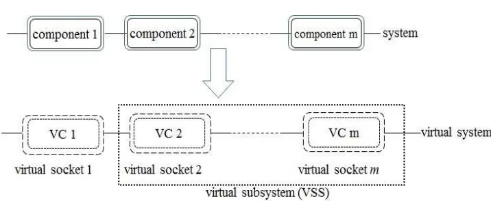
composed of two virtual components (VCs): VC1 and VC2, and the virtual series system in Model II is composed of a VC and a virtual sub-system (VSS).
Remark 1 The VC1 in Model I and the VC in Model II is replaced with an identical virtual
component (VC) upon failure of the system. The justification for this idea is as follows. For a series system with components with hazard functions hi(t) (i = 1,2, ...m), if a component
fails at tk and is replaced with a new identical one, then the contribution this new component
makes at timetk< t < tk+ 1to the CRIF of the system is Rt−tk
0 hi(x)dx. Furthermore, although
the components that fail at time points tk (k = 1,2, ...) may be different and are unknown,
the component that failed at tk has a hazard function at least as big as hc(t) = inf
1≤i≤mhi(t),
and we associate this infimum hazard function hc(t) with the virtual component. For example,
consider a series system with three components with hazard functions 0.4t, 0.45t, and 0.5t,
respectively. At τ time units following the most recent replacement, the CRIF of the system
will have a contribution that is either Rτ
0 0.4udu or
Rτ
0 0.45udu =
Rτ
0 0.4udu+
Rτ
0 0.05udu or
Rτ
0 0.5udu =
Rτ
0 0.4udu+
Rτ
0 0.1udu, and the common contribution
Rτ
0 0.4udu is the cumulative
hazard function of the virtual component. That is, the change in system reliability at each replacement is at least as big as if the most reliable component had been replaced.
In Model I, virtual component 2 (VC2) represents the remainder of the system, and in Model II the virtual sub-system (VSS) represents the remainder of the system, and at thek-th system repair VC2 and VSS are respectively not maintained and imperfectly repaired.
3.1 Model I: when the number of components is unknown unspecified
Model I is a counting process with CIF and CRIF defined as follows. Fort < t1 (prior to the first failure) the CIF of the system is Rt
0(hc(x) +λs(x))dx, and between the kth and (k+ 1)th
failure of the system (k= 1,2, . . .) the CRIF is given by
Ω1,k(t) + Ω2,k(t), (5)
where
Ω1,k(t) = Z t−tk
0
hc(x)dx
Ω2,k(t) = Z t
tk
λs(x)dx,
and hc(x) is the hazard function of VC1. The first term in (5) corresponds to VC1, which is
(virtually) replaced on failure and the second term corresponds to VC2 (the remainder of the system), on which no maintenance is carried out, so that λs(x) might for example be modelled
1 2 3 4 5 6 7 8 9 10 11 12 13 14 15 16 17 18 19 20 21 22 23 24 25 26 27 28 29 30 31 32 33 34 35 36 37 38 39 40 41 42 43 44 45 46 47 48 49 50 51 52 53 54 55 56 57 58 59 60 61
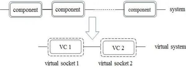
whenever the system fails, VC1 is replaced a new identical VC. We use Figure 1 to illustrate our idea. Here, VC1 has the CRIF Ω1,k(t) and VC2 has the CRIF Ω2,k(t), and Thus:
• if VC1 fails, a new identical VC will replace it and no maintenance is performed on VC2;
[image:15.612.120.420.177.287.2]• if VC2 fails, it is minimally repaired and simultaneously VC1 is replaced with a new identical VC. This means that the VC1 is replaced with a new identical VC whenever it fails or VC2 fails, so that VC1 is renewed upon system failure, regardless of which virtual component failed.
Fig. 1. The system and its corresponding virtual system in Model I.
3.2 Model II: when the number of components is known specified
Model II is a counting process with CIF and CRIF defined as follows. Fort < t1 (prior to the
first failure) the CIF of the system is Rt
0(hc(x) +λs(x))dx, and between the kth and (k+ 1)th
failure of the system (k= 1,2, . . .) the CRIF is given by
Ω1,k(t) + Ω2,k(t), (6)
where
Ω1,k(t) = Z t−tk
0 hc(x)dx,
and
Ω2,k(t) =
Rt
t1λs(x)dx if k = 1,
1
m−1
(m−k)Rt
tkλs(x)dx+
Pk−1
i=1
Rt−tk−i
tk−tk−iλs(x)dx
if 2≤k ≤m−1,
1
m−1
Pm−1
i=1
Rt−tk−i
tk−tk−iλs(x)dx if k ≥m.
Again,hc(x) is the hazard function of VC1. The first term in the CRIF of the system corresponds
to VC1, which is (virtually) replaced on failure and the second term corresponds to the virtual sub-system (VSS) (the remainder of the system).
1 2 3 4 5 6 7 8 9 10 11 12 13 14 15 16 17 18 19 20 21 22 23 24 25 26 27 28 29 30 31 32 33 34 35 36 37 38 39 40 41 42 43 44 45 46 47 48 49 50 51 52 53 54 55 56 57 58 59 60 61
whenever it fails or the VSS fails, whichever occurs first. On the VSS, we make the following remarks.
• Fort < t1, the intensity function of the VSS is denoted byλs(t), and the m−1 VCs in the
VSS are assumed to be identical and the intensity function of each VC is 1
m−1
Rt
t1λs(x)dx.
• After the first failure of the system, the VC in socket 1 is renewed and its CHF becomes Ω1,1(t) = R0t−t1hc(x)dx; the VSS has operated t1 time units and hence its CRIF becomes
Rt
t1λs(x)dx.
• After k failures (2 ≤ k ≤ m −1) have occurred, in addition to the component that has been renewed, at most k −1 VCs have been replaced since time zero. This implies that at least m−k VCs have not been replaced and the CRIF of the virtual subsystem consisting of the m−k VCs at time t is m−k
m−1
Rt
tkλs(x)dx. The exact replacement history of the other
k−1 VCs, however, is unknown, hence one may assume that VCi was installed at time tk−i
(i = 1,2, ..., k−1). The CRIF at time t of the virtual sub-system consisting of those k−1 VCs is 1
m−1
Pk−1
i=1
Rt−tk−i
tk−tk−iλs(x)dx.
• For k ≥ m, after k failures, the CRIF at time t of the m − 1 virtual components is
Rt−tk−i
tk−tk−iλs(x)dx, i= 1, . . . , m−1.
It can be seen from the above discussion that
• if the VC in socket 1 fails, a new identical VC will replace it and the oldest VC in the VSS will be renewed. No other maintenance is carried out on the other VCs in the VSS;
• if the VSS fails, the same action will be taken as when the VC in socket 1 fails. The VC in socket 1 is renewed whenever the system (which can be real or virtual) fails. The oldest VC in the VSS is replaced every k−1 failures for 2≤k ≤m−1 and is replaced every m−1 failures for k≥m, as
• On failure of the system, VC1 is replaced (renewed) and the oldest VC in the VSS is assumed to be the one replaced at the previous failure. In this way, each VC in the VSS is replaced every m−1 failures for k≥m.
[image:16.612.105.463.545.692.2]The system and virtual system are schematically illustrated in Figure 2.
1 2 3 4 5 6 7 8 9 10 11 12 13 14 15 16 17 18 19 20 21 22 23 24 25 26 27 28 29 30 31 32 33 34 35 36 37 38 39 40 41 42 43 44 45 46 47 48 49 50 51 52 53 54 55 56 57 58 59 60 61
The replacement of VCs in the VS is best illustrated by an example. In Figure 3, we show four failure times t1, t2, t3, t4 in a 3 component system. Then the virtual system is composed
of a VC and a VSS with two VCs. The three elements in the vector are the ages of the VCs immediately after replacement on failure. The first element in the vector corresponds to VC1 in the virtual system; the second and the third elements in the vector correspond to the two VCs in the VSS.
• At time t1, VC1 is replaced, VC2 and VC3 remain unchanged
• At time t2, VC1 is replaced. VC2 is assumed to be replaced at time t1, VC3 remains
un-changed;
• At timet3, VC1 is replaced. VC2 remains unchanged, VC3 is assumed to be replaced at time
t2; and
• At time t4, VC1 is replaced. VC2 is assumed to be replaced at time t3, VC3 remains
[image:17.612.75.502.300.344.2]un-changed.
Fig. 3. Failures of the virtual system corresponding a 3-component series system in Model II,showing the ages of the VCs immediately after successive system repairs.
3.3 Some properties
Let {Xk :k ≥ 1} be a sequence of nonnegative real-valued random variables with cdf Fk(t)
that have finite mean E[Xk]. To avoid trivialities, we assume thatP(Xk >0)>0. Let
Sn≡ n X
k=1
Xk, n ≥1, (7)
with S0 ≡0 and
N(t)≡max{n ≥0 :Sn≤t}, t≥0. (8)
LetFk(t) = 1−e−Ω1,k(t)−Ω2,k(t) and Xk follow cdf Fk(t).
Denote E[Nc(t)] as the renewal function corresponding to the renewal process with the
life-time distribution 1−e−R
t
0hc(x)dx.
Lemma 1 The expected cumulative number of failures in time interval (0, t] of the stochastic
process defined in Model I, denoted by E[NI(t)], satisfies
max{E[Nc(t)],
Z t
0
λs(x)dx} ≤E[NI(t)]≤E[Nc(t)] +
Z t
0
1 2 3 4 5 6 7 8 9 10 11 12 13 14 15 16 17 18 19 20 21 22 23 24 25 26 27 28 29 30 31 32 33 34 35 36 37 38 39 40 41 42 43 44 45 46 47 48 49 50 51 52 53 54 55 56 57 58 59 60 61
Proof. The system fails if either VC1 or VC2 fails. This implies the following two points.
• It is known that the reliability of a series system is smaller than the reliability of the weakest component in the system. Hence, the expected number of failures of the system up to time t
is greater than the expected number of failures of the weakest component up to timet. This proves the first inequality in Lemma (1).
• The expected number of failures of the system up to time t is smaller than the sum of the expected number of failures of VC1 and that of VC2 up to time t. This proves the second inequality in Lemma (1).
This proves Lemma 1
Lemma 1 holds as the VC in socket 1 in Model I is replaced with a new identical VC whenever it fails or the virtual system fails.
Lemma 2 Ifλs(x) is increasing inx, and hc(x) andλs(x)in Model I are the same as those in
Model II, respectively, then the expected cumulative number of failures by timetof the stochastic process defined in Model II, denoted by E[NII(t)], satisfies
E[NII(t)]≤E[NI(t)]. (10)
Proof. Note that the system in Model I is composed of VC1 and VC2, and the system in
Model II is composed of VC1 and the VSS. The two VC1s in the two systems have the same hazard function, which implies that the expected numbers of failures of these two VCs in (0, t] are equal.
On the other hand, sinceλs(x) is increasing inx, i.e.,Rt−tk−i
tk−tk−iλs(x)dx < Rt
tkλs(x)dx, it implies
that m1−1 (m−k)Rt
tkλs(x)dx+
Pk−1
i=1
Rt−tk−i
tk−tk−iλs(x)dx
<Rt
tkλs(x)dx. That is, Ω2,k(t) in Model
II is smaller than Ω2,k(t) in Model I. Hence, the expected number of failures up to time tof the
VSS in the system associated with Model II is smaller than the expected number of failures up to time t of VC2 in the system associated with Model I.
Considering both systems are series systems, we have E[NII(t)]≤E[NI(t)].
This proves Lemma 2
Lemmas 1 and 2 provide bounds on the expected number of replacements under Model I and Model II. This has practical implications for lifecycle costing, for example.
Remark 2 • Replacement occurs in socket 1 of the virtual system in both Model I and Model II whenever the system fails, even if the VC in the socket does not fail. Hence, the sequence of failures occurring at socket 1 cannot be considered a renewal process.
1 2 3 4 5 6 7 8 9 10 11 12 13 14 15 16 17 18 19 20 21 22 23 24 25 26 27 28 29 30 31 32 33 34 35 36 37 38 39 40 41 42 43 44 45 46 47 48 49 50 51 52 53 54 55 56 57 58 59 60 61
the term Ω2,k(t) = m1−1Pmi=1−1
Rt−tk−i
tk−tk−iλs(x)dx can model a state closer to equilibrium than
the state in the second and first case with CRIF= Rt
t1λs(x)dx and the state with CRIF= 1
m−1
(m−k)Rt
tkλs(x)dx +
Pk−1
i=1
Rt−tk−i
tk−tk−iλs(x)dx
. This is a useful property of Model II,
since Drenick (1960) states that the failure process of a large series system “always tends toward (statistical) equilibrium as the time of operation becomes very large”, which implies that such a failure process has two states: a transient state and an equilibrium state, as inter-preted by Meeker and Escobar (1998). Model I cannot model a failure process with two such states.
• It should be noted that the second term Ω2,k(t) in Model II (see the quantity (6)) differs
from the arithmetic reduction of intensity models proposed by Doyen and Gaudoin (2004).
The three ARI models, which are ARI∞, ARI1 and ARIm, can be re-written as λ(t) −
g(tN(t), tN(t)−1, ..., t1), where g(.) is a function of (tN(t), tN(t)−1, ..., t1). Their corresponding
CRIFs are Rt
tk(λ(x)−g(tN(t), tN(t)−1, ..., t1))dx, in which the upper limit of the integral is t,
which is different fromΩ2,k(t). In essence, the ARI models are developed for a one-component
system that is assumed to start operation att= 0. However,Ω2,k(t)in Model II is for a
multi-component system, in which the multi-components start operating at different time points.
Remark 3 When the number of components in Model II is not specified, one can fit Model II
when assuming m = 2,3, . . . and then choose m so that some model selection criterion (e.g.
AIC) is optimised.
4 Parameter estimation
Consider M independent systems of the same kind (replicates), each of which consists of
m non-repairable components with hazard functions hi(t) for i = 1, . . . , m. Suppose that Mj
failures of system j are observed at times tj,1, tj,2, . . . , tj,Mj (wherej = 1,2, ..., M), respectively.
Denote xj,1 =tj,1 and xj,k =tj,k−tj,k−1 for k ≥2 and all j.
As discussed above, for both Model I and Model II, we suppose (a) upon system failure, VC1 in both Model I or Model II is always renewed, and (b) upon system failure, VC2 in Model I follows an NHPP. For a given system j, immediately after the kth failure, the time-to-failure distribution is Fkj(t) = 1 −R1,jk(t)R2,jk(t) with R1,jk(t) = exp(−
Rt−tj,k
0 hc(x)dx)
and R2,jk(t) = exp(−Rttj,kλs(x)dx). Then the likelihood function is fj0(t)
QMj−1
k=1 fjk(t), where
fj0(t) = (hc(xj,1) +λs(xj,1)) exp
−Rxj,1
0 hc(x)dx−R
xj,1
0 λs(x)dx
1 2 3 4 5 6 7 8 9 10 11 12 13 14 15 16 17 18 19 20 21 22 23 24 25 26 27 28 29 30 31 32 33 34 35 36 37 38 39 40 41 42 43 44 45 46 47 48 49 50 51 52 53 54 55 56 57 58 59 60 61
Model I. The likelihood for Model I is
LI=
M Y
j=1
(hc(xj,1) +λs(xj,1)) exp
−
Z xj,1
0 hc(x)dx−
Z xj,1
0 λs(x)dx
×
Mj−1
Y
k=1
(hc(xj,k+1) +λs(tj,k+1)) exp −
Z xj,k+1
0
hc(x)dx−
Z tj,k+1
tj,k
λs(x)dx
!
. (11)
Model-II. The likelihood for Model II is
LII =
M Y
j=1
(hc(xj,1) +λs(xj,1)) exp
−
Z xj,1
0 hc(x)dx−
Z tj,1
0 λs(x)dx
×
"
(hc(xj,2) +λs(tj,2)) exp −
Z xj,2
0 hc(x)dx−
Z tj,2
tj,1
λs(x)dx
!#
×
m−1
Y
k=2
"
hc(xj,k+1) +
1
m−1((m−k)λs(tj,k+1) +
k−1
X
i=1
λs(tj,k+1−tj,k−i)) !
×
exp −
Z xj,k+1
0 hc(x)dx−
1
m−1 (m−k)
Z tj,k+1
tj,k
λs(x)dx+
k−1
X
i=1
Z tj,k+1−tj,k−i
tj,k−tj,k−i
λs(x)dx
!!#
×
Mj−1
Y
k=m "
(hc(xj,k+1) +
1
m−1
m−1
X
i=1
λs(tj,k+1−tj,k−i))×
exp −
Z xj,k+1
0 hc(x)dx−
m−1
X
i=1
Z tj,k+1−tj,k−i
tj,k−tj,k−i
λs(x)dx
!#)
. (12)
One can then obtain the parameters in Model I and Model II via maximising the logarithm of LI and the logarithm of LII, respectively.
5 Numerical examples
5.1 Simulation study
In this subsection, we fit Models I and II, and four other models (RP, NHPP, GP, and GRP) to artificially generated datasets, and then compare the AIC values of these models. It is known that the renewal process (RP) is usually used for perfect repair scenarios, the non-homogeneous Poisson process with power law intensity function (NHPP-PL) is often used for minimal repair, and two models for imperfect repair: the geometric process (GP) and the generalised renewal process with Vk = Vk−1 +qXk being the virtual age after the kth failure (GRP) are used for
imperfect repair. When Model I is used, the number m of components in the system is not specified.
1 2 3 4 5 6 7 8 9 10 11 12 13 14 15 16 17 18 19 20 21 22 23 24 25 26 27 28 29 30 31 32 33 34 35 36 37 38 39 40 41 42 43 44 45 46 47 48 49 50 51 52 53 54 55 56 57 58 59 60 61
(2) The time to failure of each component follows a Weibull distribution 1−e−(αt) β
, where the shape parameter β and the scale parameter α are randomly selected from the uniform distribution on the intervals (0.5, 4) and (12, 60), respectively.
(3) If a component fails, a new identical component with the same α and β as the failed one replaces the failed component.
(4) In each case we use 10 replicates of each system so that M = 10.
(5) We use the values 15, 20 for Mj, the number of failures observed for each replicate.
(6) Using the randomly generated data implied by the above, we fit each of the 6 models: the RP, the GP, the GRP, the NHPP-PL, Model I, and Model II, by maximising their respective log-likelihoods. For Model I and Model II the likelihoods are given by Eqs (11) and (12). The reader is referred to Lam (2007) for the likelihoods of the RP, the GP and the NHPP-PL, respectively, and to Yanez, Joglar, and Modarres (2002) for the likelihood of the GRP. In the RP, the GP, and the GRP, it is assumed that time to first failure
is a Weibull distribution 1−e−
t α1
β1
. In the NHPP-PL model, t α1
β1−1
is the CRIF of the series system. In both Model I and Model II, we assume that hc(t) = αβ11(αt1)β1−1 and λs(t) = βα22(αt2)β2−1.
(7) Then we calculate the AIC (Akaike information criterion) value for each model:
AIC = 2p−2 ln(L), (13)
where L is the maximized value of the log-likelihood for the model, p is the number of parameters in the model. The term 2p in the AIC penalises a model with a large number of parameters. The values of p of the six models are shown in Table 1. Note, Model I and Model II with p= 4 incur the highest penalty on their AIC values.
Table 1
The number of parameters pfor each model.
RP GP NHPP-PL GRP Model I Model II
p 2 3 2 3 4 4
WithMj = 15 andMj = 20 and m= 5,10,15 there are 6 combinations. We repeat the above
steps (1) to (7) for each of 30 repetitions, in each of which the values of α and β are different. Calculations are done with a statistical package R (which can be downloaded from www.r-project.org/). Table 2 shows the mean values and the variances (that are shown in the brackets under means) of the AIC values of the models over the 30 repetition for each combination.
1 2 3 4 5 6 7 8 9 10 11 12 13 14 15 16 17 18 19 20 21 22 23 24 25 26 27 28 29 30 31 32 33 34 35 36 37 38 39 40 41 42 43 44 45 46 47 48 49 50 51 52 53 54 55 56 57 58 59 60 61
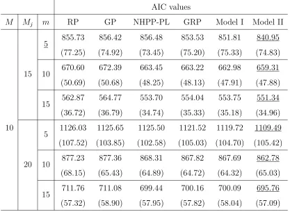
In the table, symbol ‘X’ represents the result that the hypothesis test fails to reject the null hypothesis that the AIC value of Model I (or Model II) is smaller than that of its comparison model, and symbol ‘×’ represents the result that the hypothesis test rejects the null hypothesis. From the table, we make the following observations.
• On all the comparisons, both Model I and Model II have smaller AIC values than those of the RP and the GP.
• On the performance of Model I. In only 8 out of 24 comparisons does the hypothesis test reject the null hypothesis that the AIC value of Model I is smaller than that of the NHPP-PL or that of the GRP. Thus, in the remaining 16 of the 24 comparisons the test fails to reject the null hypothesis.
• On the performance of Model II. In all the comparisons the test fails to reject the null hypothesis. That is, in all the comparisons, Model II outperforms the other models.
[image:22.612.81.498.350.655.2]• Comparing the AIC values of Model I and Model II, it can be seen that Model II outperforms Model I.
Table 2
The mean values of AIC from 30 repetitions, for various values of the number of replicates,M, number of failures Mj of each replicate, and number of componentsm in each replicate of the system.
AIC values
M Mj m RP GP NHPP-PL GRP Model I Model II
5 855.73 856.42 856.48 853.53 851.81 840.95 (77.25) (74.92) (73.45) (75.20) (75.33) (74.83)
15 10 670.60 672.39 663.45 663.22 662.98 659.31 (50.69) (50.68) (48.25) (48.13) (47.91) (47.88)
15 562.87 564.77 553.70 554.04 553.75 551.34 (36.72) (36.79) (34.74) (35.33) (35.18) (34.96)
10
5 1126.03 1125.65 1125.50 1121.52 1119.72 1109.49 (107.52) (103.85) (102.58) (105.03) (104.70) (105.42)
20 10 877.23 877.36 868.31 867.82 867.69 862.78 (68.15) (65.43) (64.89) (64.72) (64.32) (65.03)
15 711.76 711.08 699.44 700.16 700.09 695.76 (57.32) (58.90) (57.95) (57.82) (58.04) (57.09)
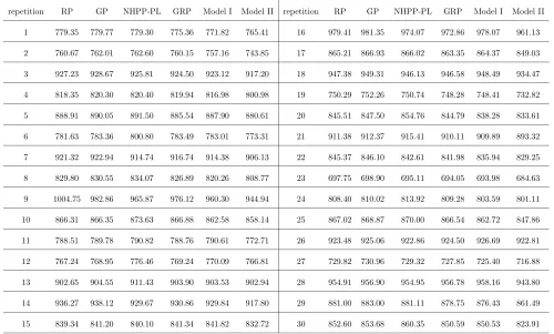
To consider further the performance of Model I and Model II, we investigate the caseM = 10,
Mj = 15, andm= 5 in more detail. The results are shown in Table 4. As can be seen from this
1 2 3 4 5 6 7 8 9 10 11 12 13 14 15 16 17 18 19 20 21 22 23 24 25 26 27 28 29 30 31 32 33 34 35 36 37 38 39 40 41 42 43 44 45 46 47 48 49 50 51 52 53 54 55 56 57 58 59 60 61
Table 3
Comparison of the AIC values of the six models based on the paired t-tests (at 5 percent level).
Is Model I’s AIC value smaller than that of Is Model II’s AIC value smaller than that of
M Mj m RP? GP? NHPP-PL? GRP? RP? GP? NHPP-PL? GRP?
5 X X X X X X X X
15 10 X X × × X X X X
15 X X × × X X X X
10 5 X X X X X X X X
20 10 X X × × X X X X
15 X X × × X X X X
(precisely, on 23 repetitions). We therefore compare the AIC values of Model I and Model II with the AIC of the GRP. Based on Table 4, we plot Figure 4 that shows the differences between the AIC values of the GRP and those of Model I (i.e., the solid line), and the differences between the AIC values of the GRP and Model II (i.e., the dashed line) on the 30 repetitions. From the figure, we make the following observations
• All the AIC differences between the GRP and Model II are positive. Thus Model II performs better than the GRP on all 30 repetitions. The largest two AIC differences are greater than 24 (i.e, the values corresponding 9 and 30 on the X-axis).
• When the AIC differences between the GRP and Model I are compared, on 10 of 30 repetitions the AIC values of the GRP are greater than that of Model I. The largest AIC difference is greater than 15 (i.e, the value corresponding 9 on the X-axis).
Furthermore, to allow the reader who may be interested to validate the results by repeating the experiment, we record model parameters generated in one of the 30 repetitions from the case in which Mj = 15 and m = 5. Table 5 shows the Weibull distribution parameters used
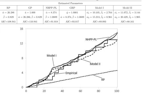
to generate the time between failures in this repetition. With these parameters, the random lifetimes of the components in a system (here M = 1) are generated (Table 6). Table 7 shows the estimated parameters and AIC for the six models. It can be seen that (1) in Model I,β2 is
smaller than 1, which implies that the hazard function λs(t) of VC2 in Model I decreases over
time, (2) the AIC values of Model I and Model II are the smallest among the six models, and (3) the values of α1 and β1 in the RP and the GP are the same and the values of α1 and β1
1 2 3 4 5 6 7 8 9 10 11 12 13 14 15 16 17 18 19 20 21 22 23 24 25 26 27 28 29 30 31 32 33 34 35 36 37 38 39 40 41 42 43 44 45 46 47 48 49 50 51 52 53 54 55 56 57 58 59 60 61
Table 4
Estimated AIC values of the six models for each individual repetition for the case when M = 10, Mj = 15 and m= 5, corresponding to the first row (with the m value underlined) in Table 2.
repetition RP GP NHPP-PL GRP Model I Model II repetition RP GP NHPP-PL GRP Model I Model II
1 779.35 779.77 779.30 775.36 771.82 765.41 16 979.41 981.35 974.07 972.86 978.07 961.13
2 760.67 762.01 762.60 760.15 757.16 743.85 17 865.21 866.93 866.02 863.35 864.37 849.03
3 927.23 928.67 925.81 924.50 923.12 917.20 18 947.38 949.31 946.13 946.58 948.49 934.47
4 818.35 820.30 820.40 819.94 816.98 800.98 19 750.29 752.26 750.74 748.28 748.41 732.82
5 888.91 890.05 891.50 885.54 887.90 880.61 20 845.51 847.50 854.76 844.79 838.28 833.61
6 781.63 783.36 800.80 783.49 783.01 773.31 21 911.38 912.37 915.41 910.11 909.89 893.32
7 921.32 922.94 914.74 916.74 914.38 906.13 22 845.37 846.10 842.61 841.98 835.94 829.25
8 829.80 830.55 834.07 826.89 820.26 808.77 23 697.75 698.90 695.11 694.05 693.98 684.63
9 1004.75 982.86 965.87 976.12 960.30 944.94 24 808.40 810.02 813.92 809.28 803.59 801.11
10 866.31 866.35 873.63 866.88 862.58 858.14 25 867.02 868.87 870.00 866.54 862.72 847.86
11 788.51 789.78 790.82 788.76 790.61 772.71 26 923.48 925.06 922.86 924.50 926.69 922.81
12 767.24 768.95 776.46 769.24 770.09 766.81 27 729.82 730.96 729.32 727.85 725.40 716.88
13 902.65 904.55 911.43 903.90 903.53 902.94 28 954.91 956.90 954.95 956.78 958.16 943.80
14 936.27 938.12 929.67 930.86 929.84 917.80 29 881.00 883.00 881.11 878.75 876.43 861.49
[image:24.612.116.461.438.656.2]15 839.34 841.20 840.10 841.34 841.82 832.72 30 852.60 853.68 860.35 850.59 850.53 823.91
1 2 3 4 5 6 7 8 9 10 11 12 13 14 15 16 17 18 19 20 21 22 23 24 25 26 27 28 29 30 31 32 33 34 35 36 37 38 39 40 41 42 43 44 45 46 47 48 49 50 51 52 53 54 55 56 57 58 59 60 61
Table 5
The parameters of the Weibull distributions of the 5 components used to generate failures in e the case Mj = 15 and m= 5.
α β α β α β α β α β
26.725 2.276 53.900 2.893 48.890 3.571 33.008 2.981 35.435 0.846
Table 6
15 observations generated using the parameters in Table 5.
8.173 3.707 2.107 14.989 2.279 4.354 5.612 8.165 7.718 0.736 7.822 11.078 9.389 3.640 10.929
Table 7
Results for the models fitted to the simulated times between failures given in Table 6. Estimated Parameters
RP GP NHPP-PL GRP Model I Model II
ˆ
α= 26.286 ˆa= 1.000 αˆ= 8.374 qˆ= 1.0001 αˆ1= 10.105,βˆ1= 2.764 αˆ1= 11.072,βˆ1= 3.144
ˆ
β= 0.829 αˆ= 26.286,βˆ= 0.829 βˆ= 1.0889 αˆ= 8.374,βˆ= 1.0889 αˆ2= 15.213,βˆ2= 0.961 αˆ2= 20.429,βˆ2= 1.905
AIC=108.941 AIC=110.941 AIC=91.018 AIC=93.017 AIC=89.093 AIC=88.161
Fig. 5. The cumulative number of failures (empirical) and the CIFs for the models fitted to the simulated times between failures given in Table 6.
5.2 A real dataset
In this subsection we compare the models when fitted to a dataset (TBF-7913) published in Proschan (1963). The data are the 27 observations of times-between-failure of an air condition-ing unit in an aircraft.
[image:25.612.53.534.218.539.2]1 2 3 4 5 6 7 8 9 10 11 12 13 14 15 16 17 18 19 20 21 22 23 24 25 26 27 28 29 30 31 32 33 34 35 36 37 38 39 40 41 42 43 44 45 46 47 48 49 50 51 52 53 54 55 56 57 58 59 60 61
be 2, 3, ..., and 10. The minimum AIC value is achieved when the number of components is 3. The parameters and the AIC values of the models are listed in Table 8, from which we can see that Model II outperforms other models.
Table 8
Results for the models fitted to the air conditioner data TBF-7913. Estimated Parameters
RP GP NHPP-PL GRP Model I Model II
ˆ
α= 79.924 ˆa= 0.971 αˆ= 73.739 qˆ= 0.0000001 αˆ1= 219.978,βˆ1= 2.988 αˆ1= 176.503,βˆ1= 1.897
ˆ
β= 1.123 αˆ= 54.917,βˆ= 1.148 βˆ= 0.988 αˆ= 49.438,βˆ= 1.123 αˆ2= 93.558,βˆ2= 1.00855 αˆ2= 77.406,βˆ2= 0.875
AIC=293.913 AIC=292.202 AIC=292.431 AIC=293.913 AIC=294.578 AIC=290.842
6 Conclusions
This paper develops two stochastic models of the failure process of a multi-component series system. Model I is designed for the case when the number of components in a system is not specified. It regards the failure process of the system equivalent to that of a virtual system consisting of two sockets into each of which there is inserted a virtual component. Whenever the system fails, replacement occurs at socket 1 and minimal repair or no maintenance is conducted on the virtual component in socket 2. Model II regards the failure process of the system equivalent to that of a virtual system consisting of a socket and a subsystem. The socket contains one virtual component and the subsystem contains m−1 sockets into each of which there is inserted virtual components. Broadly speaking, whenever the virtual system fails, replacement occurs at socket 1 and the oldest virtual component in the subsystem is replaced
virtual subsystem is imperfectly repaired.
The performance of the two models is compared with four well-known models on the basis of six artificially generated datasets. The results show that (1) overall Model I outperforms the renewal process and the geometric process on the simulated data and (2) Model II outperforms the four models on the simulated data and on the real data. Model II performs better than Model I. Furthermore, when fitted to a real-world dataset, Model II is again the best performing model of the six.
The models quantify the notion that the repair effect must be at least as big as if the most reliable component were replaced, and therefore the models consider a repair effect through component replacement rather than through the parameterization of maintenance effectiveness.
In a further applied study, we intend to fit the models to a large number of real datasets, and handle the case of right censoring in the likelihood estimation of the models. Finally, we make the point that methods that do not make parametric assumptions about the hazard function
1 2 3 4 5 6 7 8 9 10 11 12 13 14 15 16 17 18 19 20 21 22 23 24 25 26 27 28 29 30 31 32 33 34 35 36 37 38 39 40 41 42 43 44 45 46 47 48 49 50 51 52 53 54 55 56 57 58 59 60 61
consider the development of non-parametric versions of Models I and Model II.
Acknowledgements
The authors are indebted to the reviewers and the editor for their constructive comments.
References
Andersen, P. K., Borgan, O., Gill, R. D., & Keiding, N. (1993). Statistical models based on counting processes. New York: Springer Science & Business Media.
Ascher, H., & Feingold, H. (1984). Repairable Systems Reliability Modeling, Inference,
Miscon-ceptions and Their Causes. New York: Marcel-Dekker.
Asfaw, Z. G., & Lindqvist, B. H. (2015). Extending minimal repair models for repairable systems: A comparison of dynamic and heterogeneous extensions of a nonhomogeneous poisson process. Reliability Engineering & System Safety, 140, 53–58.
Baxter, L. A., Kijima, M., & Tortorella, M. (1996). A point process model for the reliability of a maintained system subject to general repair. Stochastic Models, 12(1), 12–1.
Cox, D., & Lewis, P. (1966). The statistical analysis of series of events. London: John Wiley and Sons.
Dorado, C., Hollander, M., & Sethuraman, J. (1997). Nonparametric estimation for a general repair model. The Annals of Statistics, 25(3), 1140–1160.
Doyen, L., & Gaudoin, O. (2004). Classes of imperfect repair models based on reduction of failure intensity or virtual age. Reliability Engineering & System Safety,84(1), 45–56. Doyen, L., & Gaudoin, O. (2011). Modeling and assessment of aging and efficiency of corrective
and planned preventive maintenance. IEEE Transactions on Reliability,60(4), 759–769. Drenick, R. F. (1960). The failure law of complex equipment. Journal of the Society for
Industrial & Applied Mathematics, 8(4), 680–690.
Duane, J. (1964). Learning curve approach to reliability monitoring. IEEE Transactions on Aerospace,2(2), 563–566.
Gilardoni, G. L., Toledo, M. L. G. de, Freitas, M. A., & Colosimo, E. A. (2015). Dynamics of an optimal maintenance policy for imperfect repair models. European Journal of Operational Research.
Høyland, A., & Rausand, M. (2009). System reliability theory: Models and statistical methods (Vol. 420). New Jersey: John Wiley & Sons.
1 2 3 4 5 6 7 8 9 10 11 12 13 14 15 16 17 18 19 20 21 22 23 24 25 26 27 28 29 30 31 32 33 34 35 36 37 38 39 40 41 42 43 44 45 46 47 48 49 50 51 52 53 54 55 56 57 58 59 60 61
Kijima, M., & Sumita, U. (1986). A useful generalization of renewal theory: counting processes governed by non-negative markovian increments. Journal of Applied Probability, 23(1), 71–88.
Lam, Y. (1988). Geometric processes and replacement problem. Acta Mathematicae Applicatae Sinica, 4, 366–377.
Lam, Y. (2007). The geometric process and its applications. Singapore: World Scientific. Meeker, W. Q., & Escobar, L. A. (1998). Statistical methods for reliability data. New York:
John Wiley & Sons.
Proschan, F. (1963). Theoretical explanation of observed decreasing failure rate.Technometrics, 5(3), 375–383.
Ross, S. M. (1996). Stochastic processes (2nd ed.). New York: John Wiley & Sons.
Wang, H., & Pham, H. (1996). A quasi renewal process and its applications in imperfect maintenance. International Journal of Systems Science,27(10), 1055–1062.
Wu, S., & Clements-Croome, D. (2006). A novel repair model for imperfect maintenance. IMA
Journal Management Mathematics, 17(3), 235-243.
Wu, S., & Scarf, P. (2015). Decline and repair, and covariate effects. European Journal of
Operational Research, 244(1), 219–226.
Wu, S., & Zuo, M. (2010). Linear and nonlinear preventive maintenance models. IEEE Transactions on Reliability, 59(1), 242-249.
Yanez, M., Joglar, F., & Modarres, M. (2002). Generalized renewal process for analysis of re-pairable systems with limited failure experience. Reliability Engineering & System Safety, 77(2), 167–180.

![[S974.Ebook] Free Ebook Fcked Being Sexually Explorative And Self Confident In A World Thats Screwed By Krystyna Hutchinson Corinne Fisher.pdf](data:image/gif;base64,R0lGODlhAQABAIAAAP///wAAACH5BAEAAAAALAAAAAABAAEAAAICRAEAOw==)