A new processing approach for reducing
computational complexity in cloudRAN
mobile networks
Mahmood, A, AlYasiri, A and Alani, OYK
http://dx.doi.org/10.1109/ACCESS.2017.2782763
Title
A new processing approach for reducing computational complexity in
cloudRAN mobile networks
Authors
Mahmood, A, AlYasiri, A and Alani, OYK
Type
Article
URL
This version is available at: http://usir.salford.ac.uk/id/eprint/46910/
Published Date
2018
USIR is a digital collection of the research output of the University of Salford. Where copyright
permits, full text material held in the repository is made freely available online and can be read,
downloaded and copied for noncommercial private study or research purposes. Please check the
manuscript for any further copyright restrictions.
A New Processing Approach for Reducing
Computational Complexity in
Cloud-RAN Mobile Networks
ALI M. MAHMOOD 1,2, ADIL AL-YASIRI1, AND OMAR Y. K. ALANI1
1University of Salford, Manchester M5 4WT, U.K. 2University of Technology, Iraq, Baghdad 10066, Iraq
Corresponding author: Ali M. Mahmood ([email protected])
This work was supported by the Ministry of Higher Education and the Scientific Research of Iraq–University of Technology.
ABSTRACT Cloud computing is considered as one of the key drivers for the next generation of mobile networks (e.g. 5G). This is combined with the dramatic expansion in mobile networks, involving mil-lions (or even bilmil-lions) of subscribers with a greater number of current and future mobile applications (e.g. IoT). Cloud Radio Access Network (C-RAN) architecture has been proposed as a novel concept to gain the benefits of cloud computing as an efficient computing resource, to meet the requirements of future cellular networks. However, the computational complexity of obtaining the channel state information in the full-centralized C-RAN increases as the size of the network is scaled up, as a result of enlargement in channel information matrices. To tackle this problem of complexity and latency, MapReduce framework and fast matrix algorithms are proposed. This paper presents two levels of complexity reduction in the process of estimating the channel information in cellular networks. The results illustrate that complexity can be minimized from O(N3) to O((N/k)3), where N is the total number of RRHs and k is the number of RRHs per group, by dividing the processing of RRHs into parallel groups and harnessing the MapReduce parallel algorithm in order to process them. The second approach reduces the computation complexity from O((N/k)3) to O((N/k)2.807) using the algorithms of fast matrix inversion. The reduction in complexity and latency leads to a significant improvement in both the estimation time and in the scalability of C-RAN networks.
INDEX TERMS C-RAN, Channel State Information, Computation Complexity, MapReduce, Fast Matrix Algorithms, Strassen’s Algorithm, Block LU Decomposition.
I. INTRODUCTION
Mobile networks have witnessed an unprecedented growth in terms of the number of users and the amount of data traffic. The 5G network is supposed to support 1 million user equipment (UE) per square kilometer with 1ms end-to-end latency [1]. Hence, the data rate of future 5G has been expected to be 10 times faster than the speed of 4G networks [2]. The expansion requires novel technolo-gies to be developed to meet future increased demand for mobile users. Recently, C-RAN technology has been gaining enlarged recognition from researchers and mobile network operators and has been nominated as the architecture of 5G [3]. Unlike the current mobile networks, which have the baseband unit co-located within the cell site, baseband processing in C-RAN has been moved to cloud comput-ing for central processcomput-ing and management. C-RAN has
FIGURE 1. C-RAN architecture versus distributed 4G network architecture.
FIGURE 2. Theoretical latency requirement in 4G versus the expected 1ms in 5G.
Consequently, the acquisition of CSI will affect the entire performance of cellular networks, particularly the sys-tem throughput, which ultimately limits C-RAN scalability. In this paper, two novel approaches are proposed for the C-RAN architecture to decrease the overhead of acquiring the CSI: MapReduce framework [6] and fast matrix inver-sion with multiplication algorithms. Deploying these two approaches in C-RAN will support network scalability and maintain the next generation of ultra-low latency require-ments.
The motivation and the contribution of this paper can be summarised as follows.
The most important challenges in C-RAN is the challenge of dimensionality [7]. This is due to centralized coordination of all network elements in cloud computing. In other words, the magnitude of channel matrix H in full centralized C-RAN increases dramatically at the increase in the number of RRHs and the UEs in the network. The burden of estimating this information leads to high processing time, which increases the network latency and reduces the throughput accord-ingly. However, as shown in Fig.2, in the next generation 5G networks, the target latency is 1ms, which is consid-ered a challenge and the key driver to implement the future 5G technologies (e.g. autonomous cars and tactile internet). To overcome this challenge, two novel approaches are proposed.
• The first is to deploy MapReduce as a processing
frame-work in C-RAN netframe-works to maintain low computa-tional complexity in the centralized pool of VBS, to meet the future low latency and coherence time requirements, and then to support network scalability (for large num-bers of RRHs). To the best of our knowledge, there is no prior work that has used MapReduce in the channel estimation of communication systems.
[image:3.576.39.279.67.212.2]• The second is to propose fast matrix inversion algo-rithms, to reduce the processing time of channel esti-mation in C-RAN architecture. This algorithm takes the advantage of both Strassen’s and Block LU decomposi-tion to reduce the execudecomposi-tion time of the matrix inversion of the MMSE estimator.The list of notations used in the paper is specified in Table 1, which aids in under-standing the concepts discussed in the paper. The rest of the paper is structured as follows: section II discusses some related work on the research problem outlined above. Section III demonstrates the background on the main components of the research. Section IV defines the research problem. Section V presents MapReduce as a proposed solution along with the complexity analysis and simulation results. Section VI includes a mathe-matical modeling for the MapReduce framework using queuing theory. Section VII deals with the proposed fast matrix operations algorithms (Strassen and Block LU decomposition). Section VIII illustrates simula-tion results and discussion. Secsimula-tion IX finally presents the conclusions and the possible future avenues of exploration.
TABLE 1.List of notations.
II. RELATED WORK
Another research strategy focuses on the antenna selection approaches [10]–[12], either selecting subsets or coordinating the number of active antennas. These approaches may reduce the overhead of CSI acquisition. However, the consequences might minimize the overall network capacity, because of the reduction in the number of antennas. These studies might con-sider the best case having low UE density, which requires less antennas. However, these approaches may fall short behind the provision of any improvement in worst-case scenarios, such as when having high density UEs, in busy urban areas when all antennas are required.
The authors in [13] and [14] have tried to minimize the complexity in the channel estimation algorithm itself. This involves either suggesting new estimators or modifying the current estimators. However, it has been observed that there is a trade-off between the performance (accuracy) and the com-plexity of the estimator. Many studies have tried to minimize the overhead of the most common estimator, which is the minimum mean square estimator (MMSE) by approximating the cubic complexity of matrix inversion by L-degree matrix polynomial, such as those presented in [14]–[18].
One of the trends in the research studies is to use time division duplex (TDD) systems, which utilize the channel reciprocity to reduce the overhead of the CSI acquisition. However, a TDD system has the following problems: first i) the ‘‘pilot contamination’’ is the biggest problem in TDD systems, which happens when the channel estimation at the base station in one cell becomes contaminated by users from other cells [19], [20]; ii) The same uplink/downlink timeslot arrangement must be used at all cell sites in adja-cent service areas; iii) If the TDD spectrum is divided amongst multiple operators in the same area then all oper-ators must be strictly time synchronized and have the same uplink/downlink timeslot arrangements; iv) According to the study in [21], the authors state that in the TDD systems there is still an essential need for a downlink reference signal (RS) and the uplink CSI feedback, since the measurement at the transmitter may not capture the downlink interference of the neighboring cells. Therefore, the downlink RS is still essen-tial to find the CQI for the TDD mode [21]; v) Currently the LTE licenses worldwide are less than or equal to 40 for TDD systems, while for the frequency division duplexing (FDD) systems, LTE has almost 300 more than TDD [19]; vi) a TDD system requires a large guard period for the base station to switch from downlink transmission to uplink transmission and vice versa, which leads to decline both the efficiency and the cell throughput in comparison with the FDD system, that has two separated frequencies for the uplink and down-link [22]. Hence, it is worth investigating the problem of CSI acquisition complexity in the C-RAN for the FDD systems.
In [5], [23], and [24], to decrease the overhead of CSI acquisition the authors have suggested the clustering methods in large networks, because in populated networks, the aim of obtaining CSI can be achieved by controlling the cluster size rather than the whole network. Clustering approaches can be considered as promising techniques to reduce
computational complexity. However, choosing the size and the radius of the cluster is considered as one of the main challenges. Several studies demonstrate that it is possible to implement a clustering technique for a large group of RRHs in C-RAN architecture. In the literature, clustering has been deployed for different purposes, such as for power minimiza-tion [25]–[28], and for interference mitigaminimiza-tion by using cooperative multi point (CoMP) among neighboring clus-ters [29]–[31]. Another purpose of using clustering in C-RAN is for cost reduction [32], [33] by shortening the overall fiber cable length required in the fronthaul connec-tion via deploying ring topology. Clustering is also used for complexity reduction, as in [5], [34]–[36]. This is owing to the cooperative property of C-RAN architecture, which enables full sharing of channel information by exchanging the CSI among the VBSs in the cloud. However, the focus of these studies was more on the implementation of the clustering technique, overlooking the method of processing a large number of clusters (which is formulated from a great number of RRHs). Particularly with the deployment of next generation 5G networks, there is a need for a large number of access points. For instance, the distance between two access points is expected to be less than 150 meters. Hence, an efficient and powerful processing framework is required as a processing paradigm for providing scalable distribution of hundreds or thousands of RRH groups to cope with the requirements of the next generation of mobile networks.
In this research, two novel approaches are proposed to reduce processing complexity and latency. The first approach is in managing CSI acquisition in a well distributed man-ner using MapReduce framework. The algorithm lies in the clustering category, in which a group of RRHs is chosen to be assigned to a single VBS. All other VBSs cooperate and work in a parallel manner to minimize the latency whilst maintaining the network performance. It is worth stating that MapReduce has been employed as a scalable processing paradigm to accelerate the processing of big datasets in the cloud for a large number of applications, such as scalable streaming systems, real-time prediction for explosive traffic flow data, and also, MapReduce has been used in indexing web content with the database system in the Google search engine.
Secondly, the concept of fast matrix inversion using Strassen’s algorithm and Block LU decomposition, is pro-posed to minimize the complexity in the computation of MMSE estimator.
III. RESEARCH ENABLERS
This section discusses the important components of this research: MapReduce, CSI, and common channel estimation algorithms.
A. BACKGROUND TO MapReduce
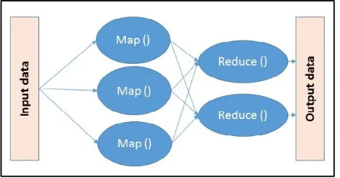
FIGURE 3. The general diagram of MapReduce framework.
MapReduce was introduced by Google [37] in order to pro-cess big data sets. Tasks are submitted initially to a division phase. Throughout this phase, the jobs include the number of tasks, mapped to a group of available mappers, for the purpose of processing. The mapper receives and produces an input and intermediate key/value pairs, respectively. The reducer takes an intermediate key and values set for that key, combining them together to form a smaller set of values. The main features of MapReduce are easy programming, auto-matic parallelism, and fault tolerance. In general, MapReduce exploits the ‘‘Divide and Conquer’’ principle. Hence, in this research instead of acquiring the channel information of all network elements (RRHs with their UEs) in one big chan-nel matrix, the estimation algorithms are applied for a pre-specified group of RRHs for each VBS using the MapReduce framework.
B. CHANNEL STATE INFORMATION IN CELLULAR NETWORKS
The mobile UE has to send its channel situation, which should be represented by the channel state information, to the base station for link adaptation between the VBS and the UE. The CSI mainly includes three reports; the precoding matrix indicator (PMI), rank indicator (RI), and channel quality indi-cator (CQI) [38]. Since adapting the modulation and coding scheme (MCS) depends on the CSI for instance, when the value channel quality indicator (CQI) (which is one of the CSI reports that are used to indicate the quality of communication link) is high, the value of MCS is also high. The RI is the number of useful transmitter antennas that can be used in the spatial multiplexing mode. The PMI is a measure that provides a preferred precoding matrix to be used in a VBS for a given radio link in spatial multiplexing mode. Hence, the former functions of the CSI reports reveal that the inac-curacy in this information leads to performance degradation in the entire mobile network.
C. SYSTEM MODEL AND CHANNEL ESTIMATION ALGORITHMS
The channel model of the received signal is presented in Equation (1). In full centralized C-RAN, the received signal in the equation for uplink transmission [5], [11],
where N represents the number of RRHs with single-antenna while K represents the number of single-antenna in UEs as follows:
YN = K
X
i=1
HiXi+Zi (1)
where, Y is the vector of the received signal; H is the channel state information matrix; X is the transmitted signal vector from K users; and Zi is the received noise vector.
In wireless communication systems, there are two common estimation algorithms, which are the MMSE and the least square (LS) estimator. The function of the estimator is to estimate the channel information (Matrix H), which includes the channel state information (CSI). The following two sub-sections present a brief description for both, the LS and MMSE estimators.
1) LEAST SQUARE ESTIMATOR
The objective of the channel LS estimator is to minimize the square value between the received signal Y and the pilot signal X. The least square estimate of the channel can be obtained by dividing the received signal by its expected value, as shown in Equation (2). The LS estimator has low com-putational complexity, since it is designed to work without any knowledge of the statistics of the channels. However, this estimator suffers from performance degradation due to the high mean square error (MSE) [14] in comparison with the MMSE, as shown in Fig.4.
ˆ HLS =
Y
X
T
=X−1Y (2)
[image:5.576.37.280.66.193.2]Where,HˆLSdenotes the estimate of channel H
FIGURE 4. Comparison between MMSE and LS estimators in terms of MSE.
2) MMSE ESTIMATOR
The statistics of MMSE estimator is represented by three auto-covariance matrices,Rgg,RYY andRHH and the
cross-covariance matrixRgY. These matrices can be calculated as
follows.
RYY =E
n
YYH
o
=xFRggFHxH+δ2nIn (3)
RHH =E
n
HHHo=FRggFH (4)
RgY =E
n
gYHo=RggFHxH (5)
Then, the estimation of the channel matrix in the MMSE estimator can be determined as follows:
gmmse =RgYR−YY1Y (6)
ˆ
Hmmse =Fgmmse=F
FHXH
−1
R−gg1δ2n+XF
−1
Y
=FRgg
FHXHXF
−1 δ2
n+Rgg
−1
F−1HˆLS
ˆ
Hmmse =RHH
h
RHH+δ2n(XXH)
−1i−1
X−1Y (7) where,
g: is the channel energy. Y: is the received signal.
F: is the discrete-time Fourier transform (DFT) matrix.
RgY: is the cross-covariance matrix of g and y.
Rgg: is the auto-covariance matrix of g.
RYY: is the auto-covariance matrix of Y.
RHH: is the auto-covariance matrix of H.
It is worth noticing that the MMSE estimator has the best performance in comparison with the LS and with other esti-mators, in terms of MSE [14], [39]. The simulation test is conducted as shown in Fig. 4 to quantify the performance of both estimators with the following key settings, 1UE and 1VBS, 4×4 antennas at UE and VBS and 1.4 BW. The result in Fig.4 shows superior performance for MMSE in compar-ison with LS. However, the main drawback of the MMSE is the high computational complexity as matrix inversion is required every time data changes [14]–[18]. Therefore, in C-RAN unlike the current mobile networks e.g. LTE-A, this computational complexity of acquiring channel information is extremely expensive and will be increased several times due to full centralized coordination on cloud computing for hundreds of RRHs which leads to huge channel information matrices. Hence, the focus of this study is to minimize the complexity of acquiring the CSI using MMSE estimator in future C-RAN architecture.
IV. PROBLEM DEFINITION
In C-RAN, the extremely large channel matrices can be con-sidered one of the main causes of the imperfection in the CSI. The detailed explanation for this problem is as follows.
After the introduction of MIMO technology, the impor-tance of accurate CSI acquisition increased, since this affects how efficiently the MIMO system works [40]. Practically,
however, when there is an increase in the number of antennas, the size of the matrix H increases and this leads to increased overheads of acquiring the CSI [34]. In the mathematical equation, the size of matrix H can be expressed by the fol-lowing equation [38], [41], [42]:
Hsize=Sc×Ns×Ar×At (8)
Where,
Sc: number of subcarriers; Ns: number of OFDM symbols;
Ar: number of receive antennas;
At: number of transmit antennas
[image:6.576.38.277.205.417.2]The number of OFDM subcarriers in the 3gpp standard is represented in Table 2 and the number of OFDM symbols is either (14 or 12) per subframe based on whether the nor-mal or extended cyclic prefix is used [38].
TABLE 2.OFDM subcarriers for uplink in each bandwidth of LTE systems [38].
[image:6.576.294.538.306.377.2]TABLE 3. The dimension of the channel matrix H against the estimation time overhead increase.
FIGURE 5. The rise of estimation time in relation to the no. of antennas.
FIGURE 6. Percentage of latency increase versus number of antennas at VBS.
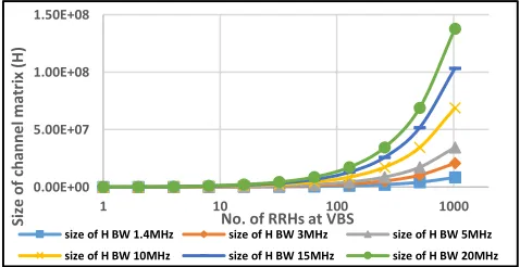
That is, with the expansion of the network size, the burden of computational complexity per user expands as well [5]. As a result, the delay of CSI leads to inaccurate decisions at the VBS. This is because the recently obtained CSI is not updated and consequently VBS does not represent the current (true) state at the mobile user. Figure 7 clarifies the problem of overheads by presenting how the increase in the dimension of H is proportional to the number of RRHs and the antennas of UEs with different channel bandwidths.
The Figures and Table above show that the magni-tude of the channel matrix increases significantly with the increase in RRHs, which eventually causes the problem of
FIGURE 7. The increase in the dimension of H with the growth in RRH for different bandwidths.
increased computation overheads and increased time taken to acquire CSI. As a result, this limits the scalability of the network.
It is worth stating that the system bandwidth is one of the important factors that also causes the growth in the dimension of matrix H as shown in equation 1, although this aspect is not within the scope of this paper. To compound this problem, the bandwidth in future networks is anticipated to increase significantly by using the white space and millimeter wave bands. Therefore, when using central processing C-RAN, a considerable amount of RRHs with their own large band-width will create a very large matrix H and the entire RRHs will yield multiple bandwidth increases. However, using the proposed MapReduce, the bandwidth will not increase in the same manner. The aggregated bandwidth is a multiple increase of the RRHs group only, not the complete number of antenna. This will definitely off-load the computational complexity in C-RAN architecture.
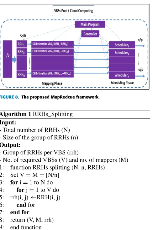
V. MapReduce DESIGN AS A SOLUTION
[image:7.576.37.279.411.544.2]FIGURE 8. The proposed MapRedcue framework.
Algorithm 1RRHs_Splitting Input:
- Total number of RRHs (N) - Size of the group of RRHs (n) Output:
- Group of RRHs per VBS (rrh)
- No. of required VBSs (V) and no. of mappers (M) 1: function RRHs splitting (N, n, RRHs)
2: Set V=M=[N/n] 3: fori=1 to N do 4: forj=1 to V do 5: rrh(i, j)←RRH(i, j)
6: endfor
7: end for
8: return (V, M, rrh) 9: end function
estimation (e.g. MMSE or LS) to acquire the CSI of the pre-specified group of RRHs. MapReduce can be deployed without the reducing phase [43]. Hence, this research amends the MapReduce framework in order to enhance its capabilities to gain the advantage of parallel processing.
The most important amendment is the use of the framework with the omission of the reducing functions, as reduction is not a prerequisite in this design. Therefore, in this work the name ‘reducing’ phase can be changed into ‘scheduling’ phase, since its main function is to schedule the estimated CSI directly to the scheduler of the VBS. The detailed description for the proposed MapReduce design is explained in Algorithms 1 and 2.
VI. ANALYTICAL DESCRIPTION TO THE OPERATION OF MapReduce USING QUEUEING THEORY
This section presents an analytical model to analyze the performance of C-RAN architecture with MapReduce using queuing theory. Two main benefits can be achieved from grouping RRHs in C-RAN using MapReduce. Firstly, it can reduce the time of acquiring the CSI, since the size of channel matrix is minimized based on the size of the group. Secondly, the network with this formulation can be scaled up without
Algorithm 2CSI Acquisition Using MapReduce in C-RAN Input:
- Y : the received signal for groups of RRHs - X : the transmitted signal vector
- Z : noise vector Output:
- The estimated H (CSI) for VBSs 1: Initialization
2: RRHs; N: no. of RRHs; K; no. of UEs per RRHs; n: group size of RRHs (n<N)
3: (V, M, rrh)=RRHs_splitting (N, n) 4: - Select Master node / Controller;
- Perform copies of user program (e.g. MMSE estimator) for (M) Mappers;
5: forid=1 to V // V: no. of VBSs
6: (data)=Read (Y, X, Z) // call for read function 7: fori=1 to n
8: forj=1 to K
9: Y(i, j)=H(i, j)∗X(i, j) + Z(i, j) 10: Data (id)=Y(i, j)
11: end for 12: end for
13: //Call MapReduce function
result=mapreduce (read, @CSIAcquisitionMapper, @ Scheduling_CSI);
14: readall (result) 15: end for
16: // Call function of Mapper (1) to Mapper (M) [from line 17, parallel processing at a time]
17: // function of Mappers 1 //apply channel estimation for VBS(1)
18: function CSIAcquisitionMapper1 (data, VBS_id) 19: { (Y, X, Z)=data
20: { find H_ estimate // using MMSE or LS 21: Add (intermKVStore,’ VBS_id ’, H_ estimate)
22: }
23: {Repeat the previous function on M mappers 24: // Call scheduling_CSI function
25: FunctionScheduling_CSI (intermKey, outKVStore)
27: // intermKey: intermediate KeyValueStore object // outKVStore: final KeyValueStore object 28: i=1 do
29: Add (outKVStore, ’VBS_id’, H_ estimate (i)) 30: While (i6=M)
31 End function
of the system for the purpose of minimizing the total costs of waiting time and then providing superior services. Likewise, using MapReduce reduces the time of CSI acquisition and this increases the system utilization via increasing the data throughput. Hence, this section will try to answer two ques-tions: i) why does the data throughput increase after using MapReduce? ii) why does the estimation time decrease after deploying the MapReduce framework?
From a queuing theory point of view, MapReduce can be represented as a multiple server queuing system (M/M/S).
For the purpose of accurate description for the pro-posed MapReduce framework in C-RAN, the following two assumptions have been considered in the calculations of the throughput and the waiting time. Firstly, both the arrival rateλ and the service rateµ are the same for all servers. This is for the purpose of fair comparison and to be compatible with the real simulation environment. Secondly, all servers are identical and have equal capabilities.
A. THROUGHPUT OF THE SYSTEM
In general, based on the principles of queueing theory, the throughput (TP) of the M/M/S can be calculated by summing the throughput or the service rateµof all servers as shown in the following formula [44]:
TPtotal_MMS=
Xm
i=1TPper−node(i)=µ1+µ2+. . .+µm (9)
The throughput of the pool of VBSs can be calculated by aggregating the throughput of all connected UEs in each VBS and then the total TP of all VBSs represents the total throughput of the pool of VBSs. The calculation of TP can be expressed in the following three equations:
TPUE(i)=B∗log 1+SINR(i) (10)
The aggregated throughput of all UEs represents the through-put per cell or VBS as follows:
TPVBS(j)=
Xz
i=1TPUE(i) (11) From equation 11, the total throughput for the pool of VBSs can be calculated as follows:
TPpool of VBSs=
Xm
j=1TPVBS(j) (12) Where,
TPUE: Throughput of the user equipment
TPVBS: Throughput of the virtual base station
TPpool of VBSs: Throughput of the pool of virtual base
stations
B: Bandwidth
SINR: Signal-to-noise-plus-interference ratio
z: Number of UEs
Before adopting MapReduce, there was a problem in the scal-ability of the VBSs because of the extremely large channel matrices, which make the acquisition of the CSI a formidable
task in C-RAN. Then, after considering the grouping tech-nique of the RRHs and parallel processing of MapReduce framework, the VBSs can be scaled-up. It is worth noting that calculating the throughput in C-RAN after adding MapRe-duce can follow similar characteristics of the multiple servers queuing system in increasing the system throughput when scaling-up the number of servers.
B. WAITING TIME
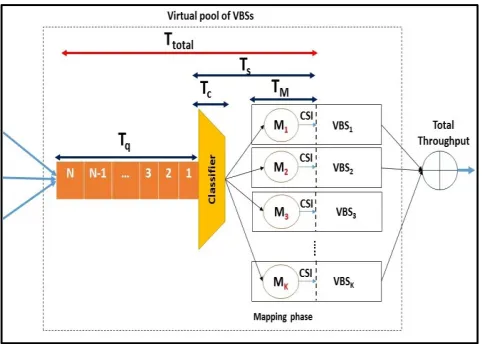
In queuing theory, the total waiting time (Ttotal) or
com-monly known as the response time [45] includes two parts as expressed in equation 13. The average waiting time in the queue (Tq) and the job service time (Ts) which is the time
required for the job to be served in the server.
Ttotal =Tq+Ts (13)
In the present design, MapReduce can be presented as a queu-ing system with multi-phase service. Therefore, the service time is divided into three phases; the classifier (Tc) or the
splitter of the incoming data, the mapping phase (TM) and
the reducing phase (TR). Hence, the total service time for
MapReduce framework can be expressed as follows:
Ts=Tc+TM+TR (14)
There is no need for the function of the reducing phase in the current design. The original reducing phase takes a set of an intermediate key-value pairs produced by the mapper as the input and runs a reducer function such as shuffling, sorting, filtering, aggregating, and combining. However, for link adaptation purposes, the VBS scheduler must directly receive the acquired CSI information at each mapper without the extra reducer stage. Therefore, the reducing phase is excluded from the current design by applying MapReduce with zero number of reducers. This can be considered as an advantageous point since the reducing phase takes addi-tional processing time and can represent a bottleneck stage in MapReduce without careful design planning [46]. Hence, the total waiting time can be represented by:
Ttotal=Tq+Tc+TM (15)
It is worth stating that the total waiting time can be affected by the number of servers, the service rate per server and the length of the queue. The rest of this section involves the mathematical representation for the component of the response time.
1) SERVICE TIME IN CLASSIFIER
The classifier is used to split the input data and send it to the servers, with a service rateβ ≥mµto avoid the case of bottleneck at the classifier, where, m is number of servers. Therefore the service time of classifier can be expressed asTc= 1β.
2) SERVICE TIME IN MAPPING PHASE
The service time (TM) for each mapper is assumed to be
FIGURE 9. M/M/1 queuing system.
two possible assumptions for determining the service time at the mapping phase, which either consider all servers as identical and have the same capabilities (therefore the service time will beαwhereα= 1
µ or if the servers have different capabilities then the service time of mapping phase can be
expressed asα=maxhµ1
1,
1 µ2, . . . ,
1 µm
i
by taking the time of the slowest server.
3) WAITING TIME IN QUEUE
For the purpose of analyzing the average waiting time in the queue (Tq), a Poisson arrivalλis considered. Three different
cases have been studied: (a) a queuing system with one server, (b) a queuing system with a number of servers equal to the number of chunks of input data, and (c) the queuing system with a number of servers less than the number of chunks of incoming data.
a: QUEUING SYSTEM WITH A SINGLE SERVER
In C-RAN the VBS that manage hundreds of RRHs can be considered a M/M/1 queue system. In the M/M/1 system the incoming data will suffer more waiting times in comparison to multi-server systems. In the case of M/M/1, the first chunk of data (N) will enter the server without waiting while the others will suffer from waiting in the queue as shown in Fig.9. Hence, the total waiting time (TWq) in the queue can be described as follows:
TWq=(N−1)∗α+(N−2)∗α+. . . .+1∗α (16)
From equation 16, the sum of positive numbers can be repre-sented by the following:
TWq=α∗ N−1
X
i=1 i
TWq=α∗
(N−1) (N−1+1)
2 =α∗
N(N−1)
2 (17)
[image:10.576.291.539.65.239.2]The average waiting time of Tq can be calculated by dividing the total waiting timeTWqby the total number of chunks of
FIGURE 10. M/M/S queue with (N=m).
input data, which is the received service.
Tq=
α∗N(N−1) 2
N =α∗
(N−1)
2 (18)
Where,αis the service time= 1
µ , hence the response time can be determined as follows:
Ttotal =Tq+TM =α∗
(N−1)
2 +α (19)
b: QUEUING SYSTEM WITH NUMBER OF CHUNKS OF ARRIVAL DATA IS EQUAL TO NUMBER OF SERVERS
In this case, the number of chunks of data (N) which represent the data from the groups of RRHs in the queuing system is equal to the number of servers (m) in the multiple server system, as shown in Fig.10. Due to the assumption above (N = m), then all the incoming N chunks of data will enter the m servers at the same time. Hence, there is no waiting time in the queue (Tq = 0). Therefore, the ser-vice time of the mapping phase requires the system to finish the processing of all data in the system, which will equal the total service time Ts. This is due to the
fact that all the data will be processed and finished con-currently. Therefore, the total time can be expressed as follows:
Ttotal=Ts =Tc+TM (20)
c: QUEUING SYSTEM WITH NUMBER OF SERVERS LESS THAN THE NUMBER OF CHUNKS OF ARRIVAL DATA (N)
The system, as shown in Fig.11, is more realistic, since in the normal condition the incoming data is more than the available servers. Therefore, the average waiting time in the queue can be calculated as follows:
According to the Figure above, the number of chunks (the number of input data N) can be expressed as follows:
FIGURE 11. M/M/S queue with (N≥K).
where,
N: number of input data in form of chunks/jobs (group of tasks) of the arrival data.
K: number of servers. b: the reminder of N/K.
a: number of times the input data has matched with the number of servers.
From the Figure above, it is noticeable that the first K chunks of data will enter the service directly without waiting in the queue: (0)δ, while the second K chunks will wait (1)δthe third K chunks will wait (2)δ and this continues for (a-1) times, whereδ is the summation of service time of classifier and mapping phase (δ=Tc+TM) Hence, the total waiting time
in the queue can be expressed as follows:
a−1
X
i=1
Kδi+abδ
But: a=N−b
K therefore, after replace (a) by N−b
K
TWq =
N−b
K
δ K N
−b K
−1+2b 2
!
TWq =
N−b
K
δN−b−K+2b
2
TWq =
N−b
K
N−K+b 2
δ (22)
For the average waiting time divide equation 24 by N
Tq= N−b
K
N−K+b 2
δ
N (23)
Therefore the overall response time can be expressed as follows:
Ttotal =Tq+Tc+TM = N−b
K
N−K+b 2
δ
N +δ (24)
The former part of this work investigated the potential of reducing the overall network computational complexity.
This has been achieved by processing data of a group of RRHs instead of the entire number of RRHs in the network. In order to complement this, the next part of this paper analyzes the computational complexity - per VBS – using a modified MMSE estimator, minimizing the execution time of the matrix inversion using fast matrix inversion by Strassen’s algorithm and Block LU decomposition.
VII. REDUCING PROCESSING TIME OF MATRIX INVERSION USING FAST MATRIX INVERSION ALGORITHMS
In the MMSE estimator, the matrix inversion was considered the main reason of its complexity [14], [18]. This section includes a novel idea of combining two algorithms, which are Block LU decomposition and Strassen’s algorithm. Both of these algorithms share the principle of dividing the matrix into sub-blocks of small matrices to find the inversion or the multiplication of matrices. Strassen’s algorithm breaks down the complexity of matrix inversion and multiplication from O(n3) to O(n2.807) [48]. Block LU also improves computing efficiency by speeding up the execution time and utilizing memory hierarchies efficiently [49]. The details of both algo-rithms are illustrated in the next sections. It is worth noting that although the reduction in complexity of matrix inversion might be small with Strassen, the reduction will be per matrix inverse. In other words, the aggregated total saving in the estimation time (ET) of the MMSE estimator will be large, since the MMSE includes more than one matrix inversion operation as shown in Equation (7).
A. STRASSEN’s ALGORITHM
In this algorithm, the matrix inversion or multiplica-tion is calculated by partimultiplica-tioning the matrix into smaller square matrices. Hence, in Strassen’s algorithm these oper-ations are applied on small sub matrices instead of apply-ing the matrix operations directly on one large matrix. In this algorithm, the matrix inversion will convert into matrix inversion and multiplication. Strassen’s algorithms for the matrix multiplication and inversion are explained as follows:
1) MATRIX MULTIPLICATION IN STRASSEN’s ALGORITHM
The matrix multiplication in Strassen’s algorithm is faster than the traditional multiplication algorithms. In the equa-tion expression, Z is the result of multiplying two square matrices X and Y, (Z=XY). According to the conventional matrix multiplication algorithms, the complexity of this mul-tiplication is O(N3) [50] while using Strassen’s method the complexity of Z will be of order O(N2.807). In the method, since the matrices are partitioned into half sized blocks, the matrices of (Z= XY) can be written in the following form:
Z11 Z12 Z21 Z22
=
X11 X12 X21 X22
Y11 Y12 Y21 Y22
Algorithm 3Strassen’s Algorithm for Matrix Multiplication Input:
Matrix X, Matrix Y, Block_size (B_S) Output:
Matrix Z, multiplication of X and Y
1: function Z=Strassen_mul(X, Y, B_S) 2: Read the dimension (n) of X
3: if dimension of n is not equal to power of 2 then 4: Error (’Enter matrix with power of 2 dimension ’)
5: End if
6: if n is less or equal to B_S
7: Z=X∗Y
8: else
9: Divide the current dimension of n,(z=n / 2) 10: Define two indexes i=1:z; j=z+1:n;
11: R1=Strassen_mul(X(i, i)+X(j, j), Y(i, i)+Y(j, j), B_S)
12: R2=Strassen_mul(X(j, i)+X(j, j), Y(i, i), B_S) 13: R3=Strassen_mul(X(i, i), B(i, j)-Y(j, j), B_S) 14: R4=Strassen_mul(X(j, j), B(j, i)-Y(i, i), B_S) 15: R5=Strassen_mul(X(i, i)+X(i, j), Y(j, j), B_S) 16: R6=Strassen_mul(X(j, i)−X(i, i), Y(i, i)+Y(i, j),
B_S)
17: R7=Strassen_mul(X(i, j)−X(j, j), YB(j, i)+Y(j, j), B_S)
18: Z=[R1+R4−R5+R7 R3+R5; R2+R4 R1+R3−R2+R6];
19: End if 20: Return (Z) 21: End function
Then the matrix multiplication can be calculated as follows:
R1 =(X11+X22) (Y11+Y22) R2 =(X21+X22)Y11
R3 =X11(Y11+Y22) R4 =X22(Y21+Y11) R5 =(X11+X12)Y22
R6 =(X21+X11) (Y11+Y12)
R7 =(X12+X22) (Y21+Y22) (26)
The overall results of matrix multiplication are:
Z11 =R1+R4−R5+R6
Z12 =R3+R5
Z21 =R+R4
Z22 =R1+R3−R2+R6 (27)
It is worth noting that, Strassen’s algorithm requires 7 multi-plications, while in the traditional multiplication algorithms requires 8 multiplications. Several researchers have stud-ied Strassen’s algorithm such as [51], [52]. The details of Strassen’s matrix multiplication algorithm is illustrated in Algorithm 3.
2) MATRIX INVERSION IN STRASSEN’s ALGORITHM
As mentioned earlier, the calculation of matrix inversion should be achieved by breaking down the matrix inversion into multiplications of several matrices. To find the inverse of Z =X−1 for a square matrix X, the matrix (X) should be divided into half sub matrices. The size of matrix X is N=m2k, where m and k are positive integer numbers and 2k is the size of the sub-matrices. Strassen’s algorithm of
matrix inversion has been studied broadly [53], [54]. The steps of Strassen’s matrix inversion can be expressed as follows:
Z11 Z12 Z21 Z22
=
X11 X12 X21 X22
(28)
Then the matrix inversion can be calculated as follows:
R1 =X11−1 R2 =X21xR1
R3 =R1xX12
R4 =X21xR3
R5 =R4−X22
R6 =R−51 (29)
The final results of matrix inversion are:
Z12 =R3xR6
Z21 =R6xR2
Z11 =R1−R3xZ21
Z22 = −R6 (30)
The algorithm for the previous equations (28, 29, 30) can be illustrated as in Algorithm 4 below. Algorithm 4 is reformu-lated from [54].
3) COMPLEXITY ANALYSIS OF STRASSEN’s ALGORITHM
The traditional matrix multiplication, such as two matrices of size (2×2) requires 8 multiplications. Hence, its complexity can be calculated as follows:
T(n)=8Tn 2
+O
n2
(31)
where, n≥2, solving Equation (31) using master theorem,
T(n)=Onlog28
=On3 (32)
Equation 34 illustrates that the complexity of traditional mul-tiplication for the smaller 2×2 matrix isO n3, while, in Strassen’s algorithm the multiplication of two matrices of size 2× 2 requires 7 multiplications, and the complexity isO n2.807.
T(n)=7Tn 2
+O
n2
(33)
T(n)=Onlog27
=On2.807 (34)
Likewise, the matrix inversion requires about 6/5(nlog27)
Algorithm 4Strassen’s Algorithm for Matrix Inversion Input:
Matrix X, Block_size (B_S) Output:
Matrix Z, Inverse of Matrix X
1: function Z=Strassen_inv (X, B_S) 2: Read the dimension (n) of X
3: if dimension of n is not equal to power of 2 then 4: Error (’Enter matrix with power of 2 dimension ’)
5: End if
6: if n is less or equal to B_S
7: Z=inv(X)
8: else
9: Divide the current dimension of n, (z=n / 2) 10: Define two indexes i=1:z; j=z+1:n 11: R1=Strassen_inv(X(i, i), B_S); 12: R2=Strassen_mul(X(j, i), R1, B_S) 13: R3=Strassen_mul(R1,X(i, j), B_S) 14: R4=Strassen_mul(X(j, i), R3, B_S) 15: R5=R4-X(j, j)
16: R6=Strassen_inv(R5, B_S); 17: Z(i, j)=Strassen_mul(R3, R6, B_S); 18: Z(j, i)=Strassen_mul(R6, R2, B_S) 19: Z(i, i)=R1-Strassen_mul(R3, Z(j, i), B_S) 20: Z(j, j)=-R6
21: End if 22: Return (Z) 23: End function
matrix inversion is considered the same as the matrix mul-tiplication O(n2.807). Details of the derivation of Strassen’s inversion complexity is explained in [55]. In conclusion, Strassen’s algorithm is faster than the traditional methods.
4) CHALLENGE OF STRASSEN’s ALGORITHM
The main challenge in Strassen’s algorithm is that the dimen-sion of the matrix X must be of order of 2k, where, k is an inte-ger [17]. Therefore, this might be the main reason that makes this algorithm uncommon for the mathematical operations of matrices. On the other hand, the dimension of the channel information matrices, where we need to reduce complexity is not always of power 2. Hence, in this research, two methods have been studied to generalize Strassen’s algorithm. These methods are illustrated as follows:
a: INCREASING THE DIMENSION OF MATRIX TO THE NEXT HIGHER POWER OF 2
As mentioned earlier, to use Strassen’s algorithm, the dimen-sion of matrix must be a power of 2. Hence, to solve this limitation, it can scale up the size of matrix to the next power of 2 by adding rows and columns of zeros with ones on the main diagonal at the end of the input matrix. This can be achieved using the Matlab function ‘‘nextpow2(n)’’ which returns the next power of 2. The following algorithm and numerical example clarify the operation of this technique.
Algorithm 5Generalization of Strassen’ Algorithm Using Next Power of 2
Input:
Matrix M, Block_size Output:
Inverse of M, (M−1)
1: Read matrix M
2: Check the dimension (n) of M
3: if dimension (n) of M is not a power of 2 4: //Check if M is a square matrix
5: if size(M,1)∼ =size(M,2)
6: error(’The matrix must be square.’)
7: end if
8: Scaling up the size of M to the next power of 2 9: Set 1 for the main diagonal
10: Set 0 for the additional rows and columns 11: M−1=Strassen_inv (B, Block_size); 12: Return the original size of M
13: Return (M−1) 14: End if
b: NUMERICAL EXAMPLE
M is a matrix of dimension 5x5 as shown below. Then to find the inverse of M by using Strassen’s algorithm, the steps in Algorithm 5 above are applied as follows.
M =
1 2 5 7 8
3 2 7 2 1
5 1 2 6 9
2 2 4 5 6
9 7 1 5 2
M =
1 2 5 7 8 0 0 0
3 2 7 2 1 0 0 0
5 2 7 2 1 0 0 0
2 2 4 5 6 0 0 0
9 7 1 5 2 0 0 0
0 0 0 0 0 1 0 0
0 0 0 0 0 0 1 0
0 0 0 0 0 0 0 1
Then the next power of 2 after 5 is 8, hence, the size will beM1−1 andM−1, as shown at the bottom of the next page.
FIGURE 12. Network performance using Strassen with next power of 2.
Strassen’s algorithm with the technique of next power of 2. The degradation in the performance comes from enlarging the original size of the matrix into a larger size of power of 2. In the next section, the block LU decomposition is proposed as a novel idea to tackle the problem of dimensions in Strassen’s algorithm. It is worth stating that in 5G networks the target end-to-end latency is 1ms as mentioned earlier. Hence, any reduction in the estimation time will contribute to the overall latency minimization.
B. GENERALIZATION OF STRASSEN’s ALGORITHM USING BLOCK LU DECOMPOSITION
Block LU decomposition is an approach used to speed up the operation of matrices [56]. The idea is to break down the high computation overhead of the big matrix into a set of smaller blocks of sub-matrices. The Block LU is used in this research for the purpose of generalization of Strassen’s algorithm, which requires the dimension of power 2. It is possible to make the size of the block of sub-matrices equal to power of 2 (n=2k) through Block LU, to fit with the requirement of Strassen’s algorithm. The Block LU method is an improve-ment to the standard LU factorization approach. In Block LU decomposition, the operations of matrix inversion or multi-plication start after dividing the upper and lower triangular into sub-blocks of small matrices. As a result of this division,
the length of the operations vectors will reduce from the original size of matrix N into n, which is the size of the sub-blocks. This approach has been studied extensively, such as in [57] and [58]. In general, the procedure of this approach can be classified into three main parts: partitioning of the original matrix into L and U triangular; dividing the lower and upper triangular into sub-blocks with a size of n; and then finding the inverse of each block and augmenting the results of sub matrices to determine the inverse of the original matrix. The details of Block LU decomposition and the combination of both Block LU- Strassen’s algorithms will be explained in the following sections.
1) PART 1 (MATRIX DECOMPOSITION INTO L AND U MATRICES)
Y is a square matrix with order N, the decomposition of Y into a product of two upper and lower matrices (Y=LU) is illustrated in equation (35) below:
y11 y12 ... y1N y21 y22 ... y2N y31 y32 ... y3N
...
yN1 yN2 ... yNN
= l11 l21 l22 l31 l32 l33
...
lN1 lN2 ... lNN
u11 u12 ... u1N
u22 ... u2N
u33 ...
... uNN (35)
where: the values of the main diagonal of the lower triangular
liiare set to one and also the unwritten values at both L and U set to zeros. The rest of values can be calculated using equations 38 and 39.
uij =yij− j−1
X
z=1
ljzuzj (36)
lij =
1
ujj
(y
ij
−
j−1
X
z=1
lizuzj) (37)
M1−1 =
0.0805 0.1421 0.2151 −0.4667 0.0390 0 0 0
−0.9069 −0.3044 −0.4075 1.8667 0.0138 0 0 0 −0.0742 0.1346 −0.0264 1.8667 −0.0516 0 0 0
1.5145 0.2365 0.2340 0.1333 0.1711 0 0 0
−0.9371 −0.2327 −0.1132 1.667 −0.1258 0 0 0
0 0 0 0 0 1 0 0
0 0 0 0 0 0 1 0
0 0 0 0 0 0 0 1
M−1 =
0.0805 0.1421 0.2151 −0.4667 0.0390 −0.9069 −0.3044 −0.4075 1.8667 0.0138 −0.0742 0.1346 −0.0264 0.1333 −0.0516
1.5145 0.2365 0.2340 −2.4667 0.1711 −0.9371 −0.2327 −0.1132 1.6667 −0.1258
The pivoting matrix P is also calculated by decomposition PY instead of Y, (PY = LU) to maintain high numerical stability and accuracy; where P is a permutation matrix of the rows, which includes 1s and 0s provided that the rest of the row and the column of each 1s are zeros. P matrix has no effect on the final result of matrix inverse.
2) PART 2 (PARTITIONING L AND U INTO SUB-BLOCKS)
In this stage, the equation of the original LU factorization can be written in the form of sub matrices as follows:
p
1 0
0 p2
Y1 Y2 Y3 Y4
=
L1 0 L2 L3
U1 U2
0 U3
(38)
Hence, from equation 40 we can get the following matrices:
P1Y1=L1U1 (39)
P1Y2=L1U2 (40)
P2Y3=L2U1 (41)
P2Y4=L2U2+L3U3 (42)
Then the following steps will be followed to find the sub matrices:
1. If the size of the sub matrix Y1 reaches the desired dimension (n), then decompose Y1to find L1, U1, P1 and find theL1−1,U1−1elsewhere, continue partitioning into smaller matrices.
2. Then, calculateLˆ
2, U2 from L1, U1, Y2and Y3. 3. Then, determineYˆ =Y4− ˆL2U2, where,Lˆ2=Y3U1−1
if the dimension ofYˆ equal to n then decopmseYˆto find L3, U3, elsewhere, continue partitioning into smaller matrices.
4. Obtain L2fromP2andLˆ2.
ˆ L2 ij = 1
(U1)ii
((Y3)ij−
Xi−1
z=1
ˆ L2
iz(U1)zj) (43)
(U2)ij =
1
(L1)ii
((Y2)ij−
Xi−1
z=1(L1)iz(U2)zj) (44) After obtainingLˆ2andU2now it can findYˆ =Y4− ˆL2U2, then if the dimension ofYˆ is equal to the block size n it can be decomposed to find L3, U3. It is worth mentioning that at the stage of calculating Y1andYˆ if they are not small enough (size larger than n), the processes of partitioning and calcu-lating the intermediate sub matrices continue recursively.
3) PART 3 (AUGMENTING THE RESULTS OF SUB-MATRICES AND FINDING THE FINAL INVERSE)
The inverse of the original lower triangular L, the upper triangular U matrices can be calculated in parallel, since both of them are independent, by augmenting all the sub-matrices of L (L1, L2, L3) and U (U1, U2, U3), and obtaining the permutation matrix P by augmenting P1and P2as follows. Algorithm 6 is recalled from the Block LU algorithm in [57].
L−1=
L1−1 0 −L−1
3 L2L
−1 1 L −1 3 (45)
Algorithm 6Block LU decomposition [57] Input:
N×N square matrix Y, block size n Output:
inverse of Y−1
1: function BlockLU (Y)
2: if the order of Y equal to the block size 3: (L, U, P)=lu (Y)
4: L−1=inverse (L) 5: U−1=inverse (U)
6: else
7: Divide Y into Y1, Y2, Y3, Y4 8: (L1−1,U1−1,P1) BlockLU (Y1) 9: Calculate U2 fromL1−1, P1and Y2 10: CalculateLˆ2fromU1−1and Y3 11: CalculateYˆ =Y4− ˆL2U2 12: (L3−1,U3−1,P2) BlockLU (Yˆ) 13: Calculate L2from P2andLˆ2 14: AugmentingL1−1, L2,L3−1to find L
−1 15: AugmentingU1−1, L2,U3−1to U−1 16: Augmenting P1and P2to find P 17: End if
18: Y−1=U−1L−1P 19: Return (Y−1) 20: End function
U−1 =
U1−1 −U−11U2U3−1
0 U3−1
(46)
P =
P1 0
0 P2
(47)
Finally, the inverse of matrix Y will be:
Y−1=U−1L−1P (48)
C. BLOCK LU – STRASSEN’s INVERSION
The inversion of Strassen’s algorithm is faster than the tra-ditional inverse algorithms used in tratra-ditional MMSE, since the complexity has been reduced into O(N2.807). In this work, and to generalize Strassen’s algorithm, the Block LU decom-position is proposed with modification. The idea is to use Strassen’s inversion as the core of the Block LU decomposi-tion instead of tradidecomposi-tional inversion, as shown in Algorithm 7. The proposed algorithm will ensure lower complexity and hence lower latency compared with Algorithm 6.
VIII. SIMULATION RESULTS AND DISCUSSION
This section is divided into two parts. The first part presents the results for deploying the MapReduce framework in the C-RAN network. The second part contains results for imple-menting fast matrix algorithms in the MMSE. This paper applies MATLAB R2016a to run the simulation tests. The simulation parameters setting are illustrated in Table 4.
Algorithm 7The proposed Block LU – Strassen Input:
N × N square matrix Y, block size(B_S) = 2∧L, L: is integer no.
Output: inverse of Y−1
1: function BlockLU (Y)
2: if the order of Y equal to the block size 3: (L, U, P)=lu (Y)
4: L-1=Strassen_inv (L, B_S) 5: U-1=Strassen_inv (U, B_S)
6: else
7: Partition matrix (Y) into (Y1,Y2,Y3,Y4) 8: (L1−1,U1−1,P1) BlockLU (Y1)
9: Calculate U2 fromL1−1, P1and Y2 10: CalculateLˆ2fromU1−1and Y3 11: CalculateYˆ =Y4− ˆL2U2 12: (L3−1,U3−1,P2) BlockLU (Yˆ) 13: Calculate L2from P2andLˆ2
14: AugmentingL1−1, L2,L3−1to find L−1 15: AugmentingU1−1, L2,U3−1to U−1 16: Augmenting P1and P2to find P 17: End if
[image:16.576.43.284.64.381.2]18: Y−1=U−1L−1P 19: Return (Y−1) 20: End function
TABLE 4. Simulation parameters.
[image:16.576.299.538.65.197.2]are presented. At the start, to quantify the amount of high computational complexity for large channel matrices on the performance of the network, the first simulation test is con-ducted with 64 and 128 antennas at one VBS using MMSE estimator with 1.4 MHz bandwidth. To establish a logical line of reasoning, one should note that in this work, the RRH is deployed with a single antenna, therefore the words antenna and RRH are alternated to describe the same concept. For the purpose of comparison, the test has been repeated using perfect channel estimation. As shown in Fig.13, the results reveal that the MMSE and the perfect channel estimation differ significantly in terms of data throughput. The perfect estimation or the theoretical estimation process means that no previous acquisition processing is necessary because of the perfect knowledge of CSI at the VBS. Consequently, unlike the real estimator (MMSE), the perfect estimator eradicates
[image:16.576.299.538.250.373.2]FIGURE 13. Test in above figure shows the effect of expansion on the cell throughput with (64 and 128 antennas) per VBS. using MMSE and perfect estimation algorithm.
FIGURE 14. Throughput per pool of VBSs (group of VBSs with 8 RRHs) using MapRedcue.
the issue of high computation overhead in obtaining the CSI with a large number of antennas in the VBS. The subsequent test uses the distributed processing in the C-RAN architecture to reduce the computation complexity faced with a large number of antennas.
The aim of deploying MapReduce is to switch the tech-nique of processing in C-RAN from centralized to a dis-tributed one. This reduces the size of H and minimizes the acquisition time of the CSI.
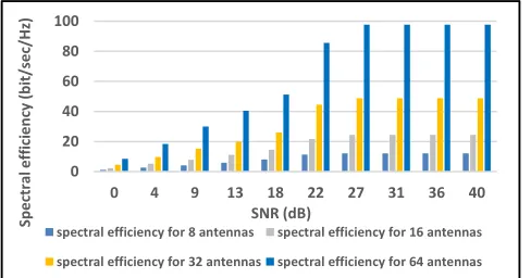
Figure 14 shows the possibility of expanding the num-ber of antennas without raising the computation overhead, while keeping the performance of the network the same for data throughput. While Fig.15 illustrates the increase in spectral efficiency, Fig.16 shows its percentage. In other words, the scalability of C-RAN with MapReduce increases the spectral efficiency of the network as the number of dis-tributed RRHs rises. Simultaneously, the estimation time and the overall response time (RT) remain constant within the time of the applied group. This is due to processing small manageable channel matrices instead of a large matrix with high computational complexity.
[image:16.576.36.277.417.517.2]FIGURE 15. Spectral efficiency with the rise the number of antennas.
FIGURE 16. Percenatge of increase in the spectral efficiency compared to the lagacy 8 antennas system.
FIGURE 17. Total response time for three groups of 8, 16 and 32 antennas at each VBS.
when considering next generation networks that require low end-to-end latency.
[image:17.576.36.279.228.398.2]Figure 18 also demonstrates the gain in the CSI acquisition time for different groups of RRHs. The figures demonstrate
FIGURE 18. Average estimation time for different groups of antennas: 8,16,32 and 64 antennas.
that the total estimation time can be minimized when group-ing is performed. In addition, the estimation time can be limited by allocating a group of RRHs to each VBS, and this reduces the computational overhead of big channel matrices. The advantage is that it meets the low coherence time require-ments for high carrier frequencies and UE speeds, and then to improve the accuracy of the CSI, since it conveys the state of the communication link between the UEs and the VBSs. The proposed distribution approach is beneficial in the next gen-eration of 5G networks since the latency will be minimized to a significant level, as shown in Fig.2, to meet the future critical time technologies. Simultaneously, a large number of antennas can be used in a scalable manner without raising the problem of the acquisition overhead in the whole network. The advantage is that in the cloud, the data, and the CSI can be completely distributed between VBSs [27]. Therefore, instead of employing a large number of antennas /RRHs per VBS (that causes a high overhead, with MapReduce) a set of VBS with the pre-specified group of RRHs have been used to obtain the CSI.
[image:17.576.38.280.435.652.2]FIGURE 19. Reduction gain (%) in response time for different RRH groups.
FIGURE 20. Throughput of pool of VBSs (simulation vs. therotical).
the overall response time decreases proportionally. Therefore more VBSs are recommended to be added in C-RAN-based MapReduce to reduce the response time. There is a noticeable difference between the analytical and the simulation results in Fig.21.In the simulation results, there are several param-eters under consideration, and the simulation tool facilitates the calculations. While in the analytical method, for the sake of simplicity, fewer parameters have been considered in the calculations.
[image:18.576.40.274.65.247.2]Part 2 (Simulation Results of C-RAN With Fast Matrix Algorithms): Several tests are conducted to examine the proposed fast matrix algorithms. At the start, to clarify the speed of Strassen’s algorithm, a comparison in the processing time is made between Strassen’s inverse algorithm and tradi-tional inverse function. The two main points are illustrated in Fig.22, which are that: Strassen’s algorithm requires less processing time and it gives more gain in time when scaling
[image:18.576.40.276.287.483.2]FIGURE 21. Reduction in response time versus no. of processors/ mappers.
FIGURE 22. Strassen_inv versus. traditional inv. with power of 2 matrices.
FIGURE 23. gain in estimation time (%) versus no. of antennas using Blocklu-Strassen alogorithm.
up the size of the matrix. However, this test is limited to a dimension of power 2 matrices.
[image:18.576.300.535.291.419.2] [image:18.576.299.535.456.588.2]FIGURE 24. Throughput per cell for 64 antennas at the VBS with fast algorithms (Block LU+Strassen).
FIGURE 25. Throughput per cell for 128 antennas at the VBS with fast algorithms (Block LU+Strassen).
can support scalability. As the number of antennas (or equiv-alently the size of the channel matrix) increases, the gain of execution time decreases.
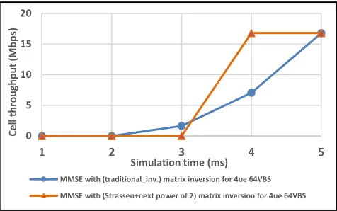
The results in Figures 24 and 25 show noticeable improve-ment in the data throughput of the network when con-sidering block LU–Strassen’s algorithms in calculating the matrix inverse in the MMSE estimator for VBSs with 64 and 128 RRHs. The reason is due to the reduction in the processing time of the matrix inversion, which leads to a reduction in the estimation time of the CSI acquisition. Therefore, the accuracy of the CSI is improved by adapting the communication channel more quickly between the UE and the VBS.
Figure 26 demonstrates a comparison of the network per-formance in terms of data throughput between the two meth-ods that have been used in this research for generalizing Strassen’s algorithm. The results show that Stassen-Block LU is more efficient, since it minimizes the initial system delay and speeds up the system response time.
The advantage of reducing the estimation time with Stassen-Block LU - particularly with the case of 64 antennas at the VBS - is that it can increase the size of the group of RRHs in MapReduce to 64 RRHs with acceptable system performance. Hence, the C-RAN network with 128, 256,
[image:19.576.300.534.247.391.2]FIGURE 26. System performance comparison between the proposed methods for generalizing Strassen’s algorithm.
[image:19.576.38.277.261.403.2]FIGURE 27. Throughput per pool of VBSs for scalable number of antennas (group of 2VBSs with 64 antennas) using MapReduce.
TABLE 5.Summary of complexity reduction.
512, 1024 RRHs can be represented with groups of 2VBSs, 4VBSs, 8VBSs and 16VBSs respectively, with 64 RRHs per VBS. For instance, Fig. 27, illustrates that 128 anten-nas can be represented by two VBSs with a group size of 64 RRHs, this scenario is not possible to implement with traditional matrix inversion due to the high execution time of matrix inversion.
It is worth mentioning that both of the proposed tech-niques (MapReduce and fast matrix algorithms) provide a considerable improvement in the reduction of computational complexity of acquiring CSI. The summary of the overall reduction is illustrated in Table 5.
IX. CONCLUSION
[image:19.576.298.537.454.528.2]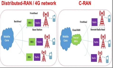
![TABLE 2. OFDM subcarriers for uplink in each bandwidthof LTE systems [38].](https://thumb-us.123doks.com/thumbv2/123dok_us/8678052.873985/6.576.294.538.306.377/table-ofdm-subcarriers-uplink-bandwidthof-lte-systems.webp)