A Bayesian approach to detect QTL affecting a simulated binary and quantitative trait

(1)

P R O C E E D I N G S

Open Access

A Bayesian approach to detect QTL affecting a

simulated binary and quantitative trait

Aniek C Bouwman

1*

, Luc LG Janss

2

, Henri CM Heuven

3

From

14th QTL-MAS Workshop

Poznan, Poland. 17-18 May 2010

Abstract

Background:We analyzed simulated data from the 14th QTL-MAS workshop using a Bayesian approach

implemented in the program iBay. The data contained individuals genotypes for 10,031 SNPs and phenotyped for a quantitative and a binary trait.

Results:For the quantitative trait we mapped 8 out of 30 additive QTL, 1 out of 3 imprinted QTL and both epistatic pairs of QTL successfully. For the binary trait we mapped 11 out of 22 additive QTL successfully. Four out of 22 pleiotropic QTL were detected as such.

Conclusions:The Bayesian variable selection method showed to be a successful method for genome-wide

association. This method was reasonably fast using dense marker maps.

Background

Discovering the genetic architecture of traits is not a tri-vial task, but it is important for our understanding of complex phenotypes. Dense marker maps make it possi-ble to perform genome-wide association (GWA) studies to detect QTL. Bayesian variable selection methods [1] are powerful in association studies, because they can simultaneous take polygenic and all SNP effects into account. This is implemented in packages such as ‘Genomic Selection’ [2] and ‘iBay’[3]. Meuwissen and Goddard [4] describe how this method could be extended to multi-trait models.

In this paper we analyzed simulated data using a Baye-sian approach implemented in the program iBay. The QTL-MAS workshop gives the opportunity to test this method on data with a QTL structure that is unknown beforehand. Although it is hypothesized that the quanti-tative and binary trait in the dataset are to some degree affected by the same QTL we used an univariate approach because the multivariate version of iBay is still in progress.

Methods Data

The pedigree contained 5 generations, all generations were genotyped but only the first 4 generations (2,326 individuals) were phenotyped for a quantitative and a binary trait. The genome consisted of 5 chromosomes and was genotyped for 10,031 SNPs. A full description of the dataset can be found at the 14th QTL-MAS work-shop website [5].

ASReml analysis

First both traits were analyzed in ASReml [6]. An animal model was applied to estimate the heritability of both traits. A bivariate animal model was applied to estimate the genetic correlation between both traits. In this bivariate analysis the binary trait was analyzed in a lin-ear model. Univariate analysis of the binary trait showed that a linear model gives similar estimates as a threshold model (results not shown).

QTL analysis

A GWA study was performed on the 2,326 individuals with phenotypes. The data was analyzed with a Bayesian variable selection method [1], implemented in iBay [3]. For QTL detection we used a model that included a

* Correspondence: [email protected]

1

Animal Breeding and Genomics Centre, Wageningen University, P.O. Box 338, 6700AH Wageningen, The Netherlands

Full list of author information is available at the end of the article

(2)

polygenic effect as well as all SNPs simultaneously. Var-iance estimates from ASReml were not used in the model. Sire-dam threshold models are required by iBay to analyze binary traits, therefore the binary trait was analyzed with a sire-dam model, while the quantitative trait was analyzed with an animal model. The following animal model was fitted for the quantitative trait:

y= +m

∑

skXk k +Z uu +e

k aa ,

and the following threshold sire-dam model was fitted for the binary trait:

y= +m

∑

a_kX_k _k + _ss+Z d_d +e

k aa Z ,

where yis the quantitative phenotype or the underly-ing liabilities of the binary phenotype for each

indivi-dual. Terms s_kX_kaa_k

k

∑

fit marker association effects where aa_k is a vector with allele substitution effects,

with aak~ N(0, I); Xk is the incidence matrix relating

allele substitution effects to observed marker genotypes and sk is a scaling factor that shrinks allele effects and models the variance explained by the marker. The scal-ing factors are conditionally estimated as simple nor-mally distributed regressions, and can be interpreted as a standard deviation.Zu,Zsand Zdare known incidence

matrices relating observations to random genetic effects

u, with u~N

(

0,As_u2

)

, sires, with s~N

(

0,Asu2

)

,

and damd, with d~N

(

0,As_u2

)

, respectively.Ais the

numerator relationship matrix, for the sire-dam model the progeny was not included in the relationship matrix.

The error vector is e~N

(

0,Ise2

)

, with identity matrix

I.

In iBay shrinkage of allele effects, through scaling fac-torss_k, is done in a dualistic manner by applying a mix-ture distribution on scaling factors that heavily shrink the effects for most of the markers, effectively removing most of the markers from the model. Only a small part of marker effects are less severely shrunken, identifying markers with important associations. This prior mixture distribution is a mixture of a normal and a truncated normal distribution:

where the first distribution is referred to as the‘null’ distribution that models the majority of markers with

no effect using π0 = 0.95 and setting sg02 to a small

value. Here sg02 was set to 0.015 for the quantitative

trait and to 0.005 for the binary trait (‘null’ markers explain ~2% of phenotypic variation,

~ ( .0 02*s_p2) / ( ₀*number of markers). The second distribution models markers with important effects. For this second distribution a truncated normal is used so that the signs of estimated allele effects will

be identifiable, and the parameter sg12 is estimated from

the data, using a flat prior. In this caseπ0/π1was set at

0.95/0.05.

For the mixture prior, the model estimates a‘mixture indicator’ which indicates for each marker whether it was estimated to belong to the first distribution or the second distribution. The first distribution is indicated by 0 and the second one with 1, so that, after averaging in the MCMC, a value ranging from 0 to 1 which is a pos-terior probability for each marker to have a large effect (i.e. the probability to belong to the second distribution) and can be used for model selection [1].

Applied MCMC techniques

All samplers were single site Gibbs samplers. The parti-cular parameterization with scaling factors was chosen so that scaling factorsskcan be sampled as‘regressions’

from normal distributions (N(0,1)) and with normal prior distributions.

Multiple MCMC chains of 50,000 cycles with a burn-in period of 1,000 cycles were run until the estimated effective number of samples was >100 for all parameters. The estimated effective number of samples was used as convergence diagnostic based on comparison of within and between chain variances.

Identification of associated markers

As indicated above, the posterior probability for a marker to come from the second mixture distribution can be used for model selection. We used two approaches to determine a cut-off on these posterior probabilities for the selection of significant associa-tions, denoting the estimated posterior probability by p_iand the prior probabilities used in the model byπ₀ andπ₁.

Analogous to the computation and use of the Bayes Factor between two models we used a ‘parameter-wise Bayes Factor’(pwBF) as the odds ratio between posterior and prior probabilities for an individual marker:

(3)

Using guidelines by Kass and Raftery [7] to judge Bayes Factors, a value above 3.2 is ‘substantial’, a value above 10 is ‘strong’, and a value above 100 is ‘decisive’.

Post-marker analysis

Using a simultaneous fit of all markers as in the Baye-sian variable selection method can cause the signal of a QTL to be spread over multiple markers. In that case individual marker have a moderate posterior probability, but the group of markers has a high joint posterior probability. The primary joint Gibbs sam-ples for the mixture indicators were used, which take account of the switches for adjacent markers being on or off, to derive the joint probability for having a sig-nal in a window. Different grouping-windows with size of 1 up to and including 11 SNP in a window were tried on the output. First, a probability for the presence of a QTL at all is given. Secondly, if there is a QTL present in the window, the probability of mul-tiple QTL in the window is given. If the mixture indi-cators show that more than one SNP within a window has a high probability of being in the model, this is counted to determine the probability of multi-ple QTL.

Results ASReml

Table 1 shows phenotypic variance and genetic para-meters for both traits. The bivariate analysis of the traits showed a positive genetic correlation of 0.66 between the traits.

iBay

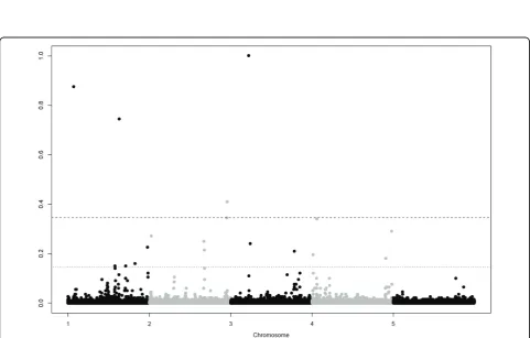
GWA for the quantitative trait resulted in 9 significant and 16 putative SNPs, the GWA for the binary trait resulted in 5 significant and 13 putative SNPs (Table 2). Figure 1 and 2 show Manhattan plots for the quantita-tive and binary trait respecquantita-tively. For both traits QTL were detected on all chromosomes, except chromosome 5, were none were simulated. Successfully mapped QTL are given in Table 3, next to the simulated details of these QTL. Mainly QTL with large effects were detected. Among the significant SNPs there was only one false positive, indicating that our threshold was

conservative, but could make a good distinction between significant and putative QTL.

Table 4 shows post-marker analysis results for both traits. Post-marker analysis showed that some regions had a probability of more than one QTL in the region.

Table 1 Phenotypic and genetic parameters for the quantitative (Q) and binary (B) trait

Trait Phenotypic variance Genetic parametersa Q 104.35 0.54

B 0.21 0.66 0.23

a

Heritabilities are on the diagonal and genetic correlation below the diagonal.

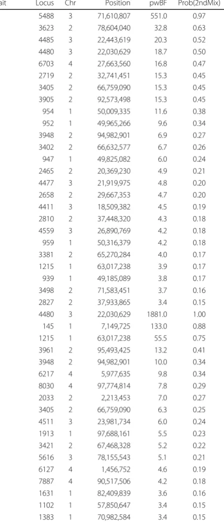
Table 2 Loci associated with the quantitative (Q) and binary (B) trait, their parameter-wise Bayes Factor (pwBF) and posterior probability (Prob(2ndMix))

Trait Locus Chr Position pwBF Prob(2ndMix) Q 5488 3 71,610,807 551.0 0.97

(4)

Figure 1Manhattanplot of posterior probabilities for the quantitative trait.Dashed and dotted lines are thresholds for significant and putative levels at parameter-wise Bayes Factor of 10 and 3.2 respectively.

(5)

Pleiotropy

Four QTL were segregating in both traits (Table 5). Pleiotropic effects of these QTL explained only 10% of the genetic correlation between the traits by including the SNPs as fixed effects in the bivariate animal model in ASReml (results not shown).

Discussion

The technique used by iBay are a Bayesian hierarchical regression model similar to Bayesian Lasso, by

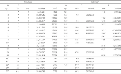
introduc-Table 3 Comparison simulated and detected QTL for the quantitative (Q) and binary (B) trait

Simulated Detectedc

Q B var Q B

QTL QTL Chr Position SNPb _QTL _SNP _Position _SNP _Position

1 * 1 7,536,081 R152 1.84 145 7,149,725 2 * 1 50,389,545 R960 1.13 959 50,316,379

3 * 1 58,038,782 R1106 1.09 1102 57,850,647 4 * 1 63,386,317 L1226 1.19 1215 63,017,238 1215 63,017,238 5 * 2 2,289,495 R2036 0.97 2033 2,213,453 6 * 2 30,511,220 L2675 0.48 2658 29,667,353

8 * 2 67,248,417 L3414 0.87 3405 66,759,090 3421 67,468,328 11 * 2 94,680,408 L3946 0.40 3948 94,982,901 3948 94,982,901 12 * 2 95,449,160 R3959 1.13 3961 95,493,425 14 * 3 22,415,527 L4483 4.50 4485 22,443,619 4480 22,030,629 17a 3 71,610,807 5488 4.49 5488 71,610,807

18 * 3 78,153,081 R5616 0.29 5616 78,155,543 22 * 4 6,296,223 R6224 0.57 6217 5,977,635 24 4 26,749,857 R6684 0.14 6703 27,663,560

30 * 4 97,651,414 R8024 0.72 8030 97,774,814 31a _Epi ₁ _49,185,089 ₉₃₉ _7.01 ₉₃₉ _79,185,089

32a _Epi ₁ _50,316,379 ₉₅₉ ₉₅₉ _50,316,379

33a _Epi ₂ _32,617,381 ₂₇₁₅ _4.18 ₂₇₁₉ _32,741,451

34a _Epi ₂ _33,139,075 ₂₇₂₇ ₂₇₁₉ _32,741,451

36a Imp 2 78,604,040 3623 2.20 3623 78,604,040

* QTL had pleiotropic effect (affected also binary trait)

Epi: epistatic QTL pair 1 (31-32) and 2 (33-34), only affecting the quantitative trait Imp: paternally imprinted QTL, only affecting the quantitative trait

a

QTL was on chip b

Closest SNP to the right (R) or left (L) of the QTL c

QTL were considered detected if the position was within 1Mbp from the simulated QTL.

Table 4 Post-marker analysis of the quantitative (Q) and binary (B) trait

Trait Region Sizea _Pr(_≥₁₎b _Pr(>1)c _{Marker start} _{Marker end}

Q 5 1.00 0.25 946 950 1 1.00 0.00 5488 5488 6 0.96 0.11 4479 4484 10 0.78 0.22 951 960 10 0.78 0.15 3901 3910 5 0.76 0.25 4485 4489 9 0.60 0.00 6696 6704 B 1 1.00 0.00 4480 4480 3 1.00 0.19 4482 4484 9 0.88 0.05 137 145 10 0.86 0.08 1207 1216

a

different grouping-windows with size of 1 up to and including 11 SNP were analyzed, region size is the number of SNPs in the window

b

probability of presence of a QTL in the region c

probability of more than one QTL in case there was a QTL present in the region

Table 5 Pleiotropic SNPs and their parameter-wise Bayes Factors (pwBF) for the quantitative (Q) and binary (B) trait

(6)

tion of a variance parameter per marker, and a model using a mixture model following the version of the Bayesian variable selection method by George and McCullogh [1]. The SNP variance originates from a mixture of two distributions, one for the SNP with an effect on the phenotype and the other for SNPs without an effect on the phenotype. The method is similar to BayesB [8]. However, BayesB uses an informative prior which is estimated from the data, in contrast iBay uses a fixed prior.

For the quantitative trait we ran 6 MCMC chains of 50,000 cycles with a burn-in period of 1,000 cycles. One chain took approximately 2.5 hour on a dual core Intel 2.33 GHz processor, so in total it took 15 hours. For the binary trait only 4 MCMC chains were needed, which took 10 hours.

A univariate QTL analysis was performed on the simulated data. However, a multivariate QTL analysis would increase the power and the precision of the pleio-tropic QTL position [9,10]. Multivariate analysis is espe-cially beneficial when one of the traits has a low heritability [10]. The simulated data contained two traits with relatively high heritabilities, therefore, the univari-ate analysis was able to detect the main QTL for either trait. A multivariate analysis might be able to detect the pleiotropic QTL with small effects as well.

Conclusions

The Bayesian variable selection method showed to be a successful method for GWA. This method was reason-ably fast using dense marker maps. The univariate Baye-sian analysis was able to detect the main QTL, however, a multivariate approach might be able to detect more pleiotropic QTL and to a more precise position.

Acknowledgements

This article has been published as part ofBMC ProceedingsVolume 5 Supplement 3, 2011: Proceedings of the 14th QTL-MAS Workshop. The full contents of the supplement are available online at http://www.

biomedcentral.com/1753-6561/5?issue=S3.

Author details

1_{Animal Breeding and Genomics Centre, Wageningen University, P.O. Box}

338, 6700AH Wageningen, The Netherlands.2_{Aarhus University, DJF}

Department of Genetics and Biotechnology, P.O. Box 50, 8830 Tjele, Denmark.3_{Clinical Sciences of Companion Animals, Faculty of Veterinary}

Medicine, Utrecht University, P.O. box 80163, 3508 TD Utrecht, The Netherlands.

Authors’contributions

ACB analyzed data and wrote manuscript. LLGJ developed software (iBay), participated in project design and coordination. HCMH conceived project, participated in project design, coordination and revising the manuscript.

Competing interests

The authors declare that they have no competing interests.

Published: 27 May 2011

References

1. George EI, McCulloch RE:Variable Selection Via Gibbs Sampling.JAMA

1993,88:881-889.

2. Calus MPL, Veerkamp RF:Accuracy of breeding values when using and ignoring the polygenic effect in genomic breeding value estimation with a marker density of one SNP per cM.Journal of Animal Breeding and Genetics2007,124:362-368.

3. Janss LLG:iBay manual version 1.47.Janss Biostatistics, Leiden, Netherlands; 2009.

4. Meuwissen THE, Goddard ME:Mapping multiple QTL using linkage disequilibrium and linkage analysis information and multitrait data.

Genet. Sel. Evol.2004,36:261-279.

5. QTL-MAS 2010 dataset.[http://jay.up.poznan.pl/qtlmas2010/dataset.html]. 6. Gilmour AR, Gogel BJ, Cullis BR, Thompson R:ASReml User Guide Release

2.0.VSN International Ltd, Hemel Hempstead, HP1 1ES, UK; 2006. 7. Kass RE, Raftery AE:Bayes Factors.JAMA1995,90:773-795.

8. Meuwissen TH, Hayes BJ, Goddard ME:Prediction of total genetic value using genome-wide dense marker maps.Genetics2001,157:1819-1829. 9. Knott SA, Hayley CS:Multitrait least squares for quantitative trait loci

detection.Genetics2000,156:899-911.

10. Sørensen P, Lund MS, Guldbrandtsen B, Jensen J, Sorensen D:A comparison of bivariate and univariate QTL mapping in livestock populations.Genet. Sel. Evol.2003,35:605-622.

doi:10.1186/1753-6561-5-S3-S4

Cite this article as:Bouwmanet al.:A Bayesian approach to detect QTL affecting a simulated binary and quantitative trait.BMC Proceedings2011

5(Suppl 3):S4.

Submit your next manuscript to BioMed Central and take full advantage of:

• Convenient online submission

• Thorough peer review

• No space constraints or color figure charges

• Immediate publication on acceptance

• Inclusion in PubMed, CAS, Scopus and Google Scholar

• Research which is freely available for redistribution