Performance Analysis of Dispersion Compensation
Fiber on NRZ and RZ Modulation with Difference
Power Transmission
Robi Darwis
*, Octarina Nur Samijayani, Ary Syahriar, Indrawan Arifianto
Department of Electrical Engineering, Faculty of Science and Engineering, Al Azhar University of Indonesia, Indonesia
Copyright©2019 by authors, all rights reserved. Authors agree that this article remains permanently open access under the terms of the Creative Commons Attribution License 4.0 International License
Abstract
Optical fiber communication hascharacteristics that really need attention. The characteristics of fiber optic transmission are very important in designing optical fiber networks, one of which is widening pulses called dispersions. Dispersion is the widening of light pulses in optical fibers which reduces data speed, signal to noise ratio and system quality. In addition to dispersion compensation, which is the most important feature needed in fiber-optic communication systems; transmission power needs to be considered to produce optimal signal output. In this paper, we will simulate the optimization effect of power and fiber dispersion compensation on Non Return to Zero (NRZ) and Return to Zero (RZ) modulation on optical transmission systems, with 5 dBm power parameters, 10 dBm 15 dBm and 0 dBm and DCF 5 km, 10 km, 15 km, 20 km and 25 km. Simulation results show that dispersion compensation is very influential on the transmission system. From these two modulations, there are differences in the results between NRZ and RZ. The results of dispersion compensation also affect the input power and DCF length.
Keywords
DCF, Power Transmission, NRZ, RZ1. Introduction
The characteristics of fiber optic transmission are very important in designing fiber optic networks [1,2]. Optical communication systems also face problems such as dispersion (chromatic dispersion, polarization dispersion modes, second order and third order dispersion), attenuation and nonlinear effects that limit performance. Dispersion factors are a very dominant problem compared to others [3, 4].
Effectively dispersion speaks of widening pulses. Dispersion is the effect that is responsible for spreading the
signal when propagating. The signal is represented by pulses [5]. Dispersion is the widening of light pulses in optical fibers which reduces data speed, signal ratio to noise and system quality. The widening of this pulse leads to Inter-Symbol-Interference (ISI), where the output pulses of a system will experience interference or overlap, so the output becomes undetectable [4].
Besides dispersion compensation, which is the most important feature needed in a fiber optic communication system[6], it seems that the best solution for high attenuation is to pump more optical power or concentrate and focus on power optimization. External modulation is usually adopted. In terms of power efficiency and bandwidth efficiency, a number of the most popular modulation techniques are used [7].
Modulation techniques that are widely used in optical communication systems are generally simple modulation-based on-off keying (OOK)[8]. This paper will analyze the performance of optical systems using dispersion compensation fiber and power optimization for NRZ and RZ modulation techniques. Performance will be analyzed based on measurements of Q factor, Bit Error Rate (BER) and Eye Diagram by varying various parameters and optimize the launch power and DCF length to maximize the good quality transmissions.
2. Basic Theory
2.1. Dispersion
on the design comes from the waveguide component of total dispersion. This is the only component that can be changed significantly by the appropriate modification of the refractive index profile shape [9].
Attenuation and dispersion are the two most important effects that play a major role in fiber optic transmission systems. Attenuation of optical signals will limit the availability of optical power along the transmission path, and for very low attenuation, the dispersion limit of the repeater distance is below what is possible from attenuation factors. Fat loss has been reduced from 100 dB / km (i.e., transmission may be only a few meters) at 1,300 nm in 1970 to around 0 25 and 0 15 dB / km which is very close to transparent boundaries which may be theoretically and transmission over several hundred kilometers fiber, for the wavelength region of 1300 and 1550 nm respectively, in 1980 [9].
2.2. The Effect of Fiber Optic Dispersion on Optical Transmission
Loss and dispersion are the major factor that affect fiber-optical communication being the high-capacity develops. The EDFA is the gigantic change happened in the fiber-optical communication system; the loss is no longer the major factor to restrict the fiber-optical transmission. Since EDFA works in 1550 nm wave band, the average Single Mode Fiber (SMF) dispersion value in that wave band is very big, about 15-20ps / ( nm. km-1). It is easy to see that the dispersion becomes the major factors that restrict long distance fiber-optical transfers [3, 10, 11]. In single-mode fiber, performance is primarily limited by chromatic dispersion which occurs because the index of the glass varies slightly depending on the wavelength of the light, as the light from real optical transmitter necessarily has nonzero spectral width. Polarization mode dispersion, another source of limitation occurs because although the single-mode fiber can sustain only one transverse mode, it can be carried with two different polarizations, and slight imperfections or distortions in a fiber can alter the propagation velocities for these two polarizations [3], [10], [11]. This phenomenon is called polarization mode dispersion and Mode birefringence Bm is defined as the follow
Bm= �βx-βy�
k0
= nx-ny (1)
nx, ny are the effective refractive of the two orthogonl polarizations. For a given Bm, its fast axis and slow axis components would develop the phase difference after the light waves transmission L Km.
Φ= k0Bm L= 2πλ �Nx-Ny�L=�βx-βy�L (2)
If the Bm remains constant, the phase difference between its fast axis and slow axis will be periodically repeated. The length that leads to a phase difference of 2π
or power periodic exchange is called polarization beat length:
L= 2π
�βx-βy� = λ
Bm (3)
If the incident light has two polaization components, due to refactive difference between the fast axis and slow axis, the tansmit rate of two polaization components will be different. Because the randomness of fiber birefingence changes, the group velocity of different polaization direction is also random, and this will result in the outut pulse broadening. Degee of pulse broadening can be expressed by different group delay ∆T.
∆τ
=
�VL gx–
L Vgy�
=
d
dω�βx-βy�L
=
�nx-ny
c
+
ω c
d(nx-ny)
dc �L (4)
From the equations present that the initial pulse is broadened by the transmission. The longer the optical signal transmission distance, the geater the fiber dispersion coefcient, the more pulse broaden. The two adjacent pulses result overheating, error judgment will generated [10, 11].
The influence of dispersion on system performance is also reflected in the optical fiber nonlinear effects. Dispersion increased the pulse shape distortion caused by the self-phase modulation dispersion (SPM); on the other hand, dispersion in WDM systems can also increase the cross-phase modulation, four-wave mixing (FWM) and other nonlinear effects [10-12].
2.3. DCF Dispersion Compensation Technology
In order to improve overall system performance and reduced as much as possible the transmission performance influenced by the dispersion, several dispersion compensation technologies were proposed [6]. Amongst the various techniques proposed in the literature, the ones that appear to hold immediate promise for dispersion compensation and management could be broadly classified as: dispersion compensating fibers (DCF), chirped fiber Bragg gratings (FBG) and high-order mode (HOM) fiber [10], [13].
The idea of using dispersion compensation fiber for dispersion compensation was proposed as early as in 1980, but it was not until the invention of optical amplifiers that DCF began to receive attention and be studied. As products of DCF are more mature, stable, not easily affected by temperature and wide bandwidth, DCF has become a most useful method of dispersion compensation [13].
∂Aj(z,t)
∂z + 1 2iβ2�λj�
∂2A j(z,t)
∂t2 -iγ�Aj(z,t)� 2
Aj(z,t)+ α
22Aj(z,t)=0 (5)
Aj(z,t) is complex amplitude of j channel optical pulse, 𝛽𝛽2(λi) is the dispersion parameter of j channel, γ is the nonlinear co-efficent, α is the loss co-efficient. After N-section dispersion compensation of DCF, the channel residual dispersion can be expressed as:
∆D�λj�= NLSMF��1-μp�DSMF�λp�+(j-p)∆λ(
dDSMF�λp�
dλ
-μpDSMF�λp�
DDCF�λp�
dDSMF�λp�
dλ )� (6)
In the formula, μp is the dispersion compensation rate of p-channel.
μp=�DDCF(λp)LDCF
DSMF(λp)LSMF�
(7) LSMF and LDCF are the conventional single-mode fiber length and dispersion compensation fiber length within the amplifer spacing. ∆λ is the channel wavelength spacing. DDCF (λp) and DSMF(λp) ae the dispersion coefcient of conventional single-mode fiber and dispersion compensation fber at the
λ
p wavelength[10, 11].2.4. Modulation Technique
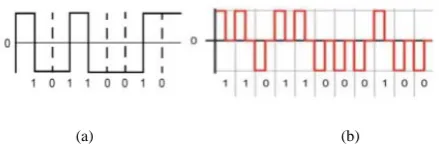
When analyzing the performance of optical communication systems, the data transmission format must be analyzed because it deals directly with the system output. Many coding techniques have been proposed before and have become standard in telecommunication and computer networks [14]. Optical modulation format is a method used to impress data on optical carrier waves for transmission through optical fibers. The simplest optical modulation format is modulation of on-off-keying (OOK) intensity, which can consist of two forms: non-return-to-zero (NRZ) and return-to zero (RZ) [15]. Return to zero (RZ) and non-return to zero (NRZ) are two very common modulation techniques, which are used to modulate optical pulses in optical networks. In a simple comparison, the NRZ modulation technique requires less bandwidth for transmission than RZ and is not sensitive to laser phase noise [16].
(a) (b)
Figure 1. (a) NRZ and (b) RZ of Optical Communication [17]
Each of these modulation schemes offers a certain optical average power, and therefore they are usually compared in terms of the average optical power required to achieve a desired BER performance or SNR. The power effciency ηp of a modulation scheme is given by the average power required to achieve a given BER at a given data rate [7]. Mathematically, ηp is defined as:
ηp=Epulse
Eb
(8) where Epulse is the energy per pulse and Eb is the average energy per bit.
3. Methodology
In this paper, we investigate the effect of the length of dispersion compensation fiber (DCF) and the optimization of power launch on the data transmission system. This study designed a simulation using two modulation techniques namely NRZ and RZ. This simulation uses Optisystem 7.0.
[image:3.595.306.535.396.542.2]The following parameters are set in this study:
Table 1. Standard Single-Mode Fiber Parameters
Parameters Values
Reference Wavelength 1550 nm
Length of Fiber 10 km
Attenuasi 0.2 dB/km
Dispersion 16.75 ps/nm/km
Dispersi slope 0.075 ps/nm2/km
Differential Group Delay 0.2 ps/km
Lower calculation limit 1200 nm
Upper calculation limit 1700 nm
Power Transmitter 5dBm, 10dBm, 15dBm, 20dBm
[image:3.595.65.285.565.643.2]This single-mode fiber can cause attenuation and dispersion in fiber transmission data. Therefore, the transmission media also requires amplifiers and DCF (Dispersion Compensating Fiber).
Table 2. Dispersion Compensating Fiber Parameters
Parameters Values
Attenuasi 0.2 dB/km
Dispersion -85 ps/nm/km
Dispersi slope -0.3 ps/nm2/km
Differential Group Delay 0.2ps/km
Lower calculation limit 1400 nm
Upper calculation limit 1700 nm
[image:3.595.306.535.628.744.2]The output of the transmission media will then be input for optical receivers.
For the above parameters, it will be analyzed how the effect of changing each power on each length of Dispersion Compensating Fiber in both RZ and NRZ modulation.
4. Result and Analysis
4.1. Results of Power Receiver in Difference Input Power and DCF Length
The table below is the result of a simulation of the effect of input power on different DCF lengths and on different modulation techniques on NRZ and RZ.
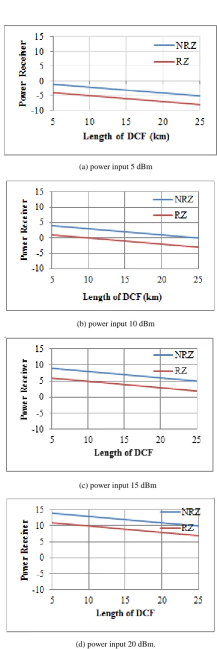
[image:4.595.312.528.58.701.2]Figure 1 shows a comparison of the power receiver to distance. The graph above is how the DCF length affects the power receiver results. It is seen that the greater the DCF distance, the smaller the power receiver.
Table 3. Power receiver results from simulations with difference power input in difference distance
Input Power
Length of DCF
(km) NRZ RZ
5 dBm
5 -1.097 dBm -4.012 dBm
10 -2.097 dBm -5.012 dBm
15 -3.097 dBm -6.011 dbm
20 -4.097 dBm -7.011 dBm
25 -5.097 dBm -8.012 dBm
10 dBm
5 3.990 dBm 0.986 dBm
10 2.990 dBm -0.012 dBm
15 1.990 dBm -1.012 dBm
20 0.990 dBm -2.012 dBm
25 -0.010 dBm -3.012 dBm
15 dBm
5 8.990 dBm 5.916 dBm
10 7.990 dBm 4.916 dBm
15 6.990 dBm 3.915 dBm
20 5.990 dBm 2.916 dBm
25 4.990 dBm 1.916 dBm
20 dBm
5 13.903 dBm 10.916 dBm
10 12.903 dBm 9.916 dBm
15 11.903 dBm 8.916 dBm
20 10.903 dBm 7.915 dBm
25 9.903 dBm 6.915 dBm
(a) power input 5 dBm
(b) power input 10 dBm
(c) power input 15 dBm
[image:4.595.60.288.349.656.2](d) power input 20 dBm.
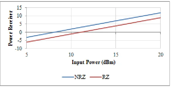
Figure 2. Graph of Power Receiver to Input power
Figure 2 shows how the power input added to the power receiver on this DCF system. From the graph above, it can be seen that the greater the input power, the more powerful the power receiver.
4.2. Q Factor and Bit Error Rate Analysis
[image:5.595.152.444.80.239.2]The following table is the result of a power optimization and dispersion compensation simulation on NRZ modulation with variations in the power delivery to each DCF length variation. This simulation produces the number of Q Factor and Bit Error Rate (BER)
Table 4. Q Factor and BER results from simulations using NRZ modulation
Power 5 km 10 km 15 km 20 km 25 km
5 dBm Q Factor 24.3869 12.2258 7.58777 4.51183 2.48181
BER 1.12e-131 1.12e-034 1.62e-014 3.21e-006 0.00649
10 dBm Q Factor 24.3628 12.8714 6.96144 4.23604 2.32612
BER 1.95e-131 3.261e-038 1.68e-012 1.135e-005 0.009945
15 dBm Q Factor 25.7458 15.3727 5.35276 3.44015 1.93778
BER 1.67e-146 1.136e-053 4.33e-008 0.0002895 0.026226
20 dBm Q Factor 11.809 6.84841 2.70905 1.90257 0
BER 1.68e-032 3.7224e-012 0.00335531 0.0284968 1
[image:5.595.69.525.370.500.2]From the table above, it can be seen that the type of power launched at different levels produces different Q Factors and BER at each distance or length of the DCF.
Table 5. Q Factor and BER results from simulations using RZ modulation
Power 5 km 10 km 15 km 20 km 25 km
5 dBm Q Factor 46.3815 19.5877 2.5202 0 0
BER 0 9.417e-086 0.00480306 1 1
10 dBm Q Factor 41.7241 17.6244 2.31997 0 0
BER 0 7.8161e-070 0.00865602 1 1
15 dBm Q Factor 29.2253 11.9276 1.81269 0 0
BER 4.61e-188 4.2426e-033 0.0318803 1 1
20 dBm Q Factor 7.27353 3.7132 0 0 0
BER 1.74e-013 9.3166e-005 1 1 1
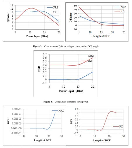
[image:5.595.72.527.552.682.2]Figure 3. Comparison of Q factor to input power and to DCF length
Figure 4. Comparison of BER to input power
Figure 5. Comparison of BER on DCF length
From table 4 and table 5, it can be analyzed that each addition of Dispersion compensating fiber will decrease the Q Factor value. The decrease in the Q Factor is due to one of the optical fiber dispersion values that accumulate when the link is getting farther away, where the positive dispersion value possessed by the SMF optical fiber accumulates positively linearly as the link length increases. The greater the accumulation of the dispersion value, the smaller delay between channels, which gives rise to a significant Inter Symbol Interference (ISI). The use of DCF optical fiber which has negative dispersion value can reduce the positive dispersion value of SMF, where it
accumulates positively linearly with increasing link length, thus increasing delay between channels that significantly reduce Inter Symbol Interference (ISI).
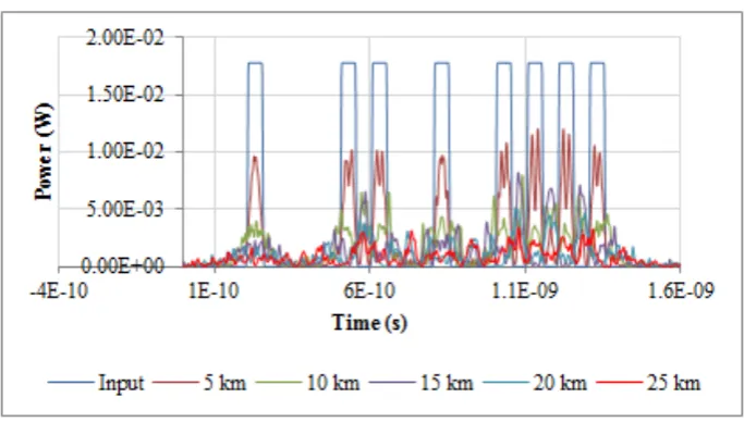
[image:6.595.83.514.83.217.2] [image:6.595.188.411.243.408.2]Figure 6. Graph of input and output with the difference of DCF length in NRZ
Figure 7. Graph of input and output with the difference of DCF length in RZ
4.3. Input and Output Analysis
Below is a graph of the input and output comparisons for each different distance. In this simulation, the input power entered is the average power of the previous test, which is 12.5 dBm with a variable length DCF variable that varies from 5 km to 25 km in multiples of 5.
Figure 6 and 7 show a comparison of the input signal and output signal in each modulation. Figure 6 shows a graph of the input and output signals on the NRZ transmission and figure 7 shows a graph of the input signal and output signal on the RZ transmission. It was seen that both experienced noise did not get a full signal on the receiver. This happens because of the effects of dispersion and noise during propagation.
5. Conclusions
Based on the above analysis, it can be concluded that by using power transmitter optimization and dispersion compensation on optical transmission systems greatly
affects system performance. The bigger the transmitter power, the Q factor will decrease and the BER will increase. As well as the addition of DCF, the Q factor will decrease and the BER will increase. Therefore power optimization and dispersion compensation fiber greatly influence the performance of the optical transmission system. Based on the replacement of the modulation technique used between Non Return to Zero (NRZ) and Return to Zero (RZ), in testing different input power NRZ produces a small Bit Error Rate than NR. In testing by varying the length of DCF even the value of BER on NRZ is smaller than RZ. These results can be concluded that NRZ is better than NZ when viewed in terms of BER.
Appendix
Bit Error Rate
[image:7.595.127.469.273.467.2]Pe = M
N+MPe1+
N
M+NPe1 (9) where P0 and P1 are the probabilities of the symbols, M is the number of samples for the logical 0, and N is the number of samples for the logical 1. Also, Pe0 and Pe1 are:
Pe0= 1 2erfc(
S-μ0
√2σ0) (10)
Pe1= 1 2erfc(
μ1-S
√2σ1) (11)
Where
µ
0,µ
1,σ
0 andσ
1 are average values and standard deviations of the sampled values respectively, and S is the threshold value.An enhancement of the simple Gaussian approximation can be achieved by averaging the separately estimated BERs for different sampled symbols [9]. For M sampled values for the logical 0 and N sampled values for the logical 1, the corresponding error rates are:
Pe1= 1
2N∑ erfc N i=1 (
μ1i-S
√2σ1i) (12)
Pe0=
1
2M∑ erfc M i=1 (
𝜇0i-S
√2σ0i) (13)
If the signal is mixed with the noise, the Average Gaussian method is modified to calculate the average error patterns. The detailed description is [14]:
Pe=∑
NP
Merfc
8
i=1 (
𝜇𝑖-S
√2σi) (14)
Q Factor
There are two modes to calculate the Q-Factor: The Q-Factor from BER is calculated numerically by:
Pe=1
2erfc( Q
√2) (15)
where the Q-Factor is calculated: Q = �𝜇1 - 𝜇0�
σ1- σ0 (16)
REFERENCES
K. Iizuka, Elements of Photonics For Fiber Integrated
[1]
Optics, 2nd ed. New York: Wiley Interscience, 2002.
G. Singh and J. Saxena, “Dispersion Compensation Using [2]
FBG and DCF in 120 Gbps WDM System,” Int. J. Eng. Sci. Innov. Technol., vol. 3, no. 6, pp. 514–519, 2014.
M. Yadav and A. K. Jaiswal, “Design Performance of High [3]
Speed Optical Fiber WDM System with Optimally Placed DCF for Dispersion Compensation,” Int. J. Comput. Appl., vol. 122, no. 20, pp. 36–39, 2015.
V. Joshi and R. Mehra, “Performance Analysis of an Optical [4]
System Using Dispersion Compensation Fiber & Linearly Chirped Apodized Fiber Bragg,” Open Phys. J., pp. 114– 121, 2016.
M. S. Wartak, Computational Photonics An Introduction
[5]
with MATLAB. New York: Cambridge University Press, 2013.
R. Udayakumar, V. Khanaa, and T. Saravanan, “Chromatic [6]
Dispersion Compensation in Optical Fiber Communication System and its Simulation,” ndian J. Sci. Technol., vol. 6, pp. 1–5, 2013.
R. Ghassemloy, Z; W, Popoola; S, Optical Wireless
[7]
Communications System and Channel Modelling with MATLAB. Londo: CRC Press Taylor And Francis Group, 2013.
D. Astharini, A. Mayola, O. N. Samijayani, and A. Syahriar, [8]
“Performance Analysis of Digital Modulation Techniques on Wireless Optical Channel,” vol. 17, no. 1, pp. 7–12, 2017.
B. H, Le, and Nguyen, Guided Wave Photonics
[9]
Fundamentals and Application With MATLAB. Australia: CRC Press Taylor And Francis Group, 2012.
B. Hu, W. Jing, W. Wei, and R. Zhao, “Analysis on [10]
Dispersion Compensation with DCF based on Optisystem,”
Int. Conf. Ind. Inf. Syst., vol. 6, no. 8, pp. 40–43, 2010.
A. B. Sarkar and K. S. Alam, “Analysis of Dispersion [11]
Compensation System for Optical Fiber Communication in a WDM Network,” Int. J. Sci. Eng., vol. 6, no. 8, pp. 1270– 1275, 2015.
S. Kumar, P. A. K. Jaiswal, E. M. Kumar, E. R. Saxena, M. T. [12]
Student, and S. Shiats, “Performance Analysis of Dispersion Compensation in Long Haul Optical Fiber with DCF,” IOSR J. Electron. Commun. Eng., vol. 6, no. 6, pp. 19–23, 2013.
Gurpreet, Navdeep, and Ranvir, [13]
“Use_of_Dispersion_Compensating_Fiber_in,” Int. J. Adv. Eng. Res. Sci., vol. 1, no. 4, 2014.
U. Jadon, H. Nain, and V. Mishra, “NRZ VS RZ : [14]
Performance Analysis of SMF with Different Laser Sources at 10 Gbps,” IEEE Int. Conf. Recent Trends Electron. Inf. Commun. Technol., pp. 43–46, 2016.
S. Gupta and N. K. Shukla, “Pre- , Post , Symmetric1 and 2 [15]
Compensation Techniques with RZ Modulation,” Int. Conf. Recent Adv. Inf. Technol., 2012.
F. E. Seraji and M. S. Kiaee, “Eye-Diagram-Based [16]
Evaluation of RZ and NRZ Modulation Methods in a 10 - Gb / s Single-Channel and a 160 - Gb / s WDM Optical Networks,” vol. 7, no. 2, pp. 31–36, 2017.
Z. Ibrahim, C. B. M. Rashidi, S. A. Aljunid, A. K. Rahman, [17]