Dynamic load forecasting for commercial power network

(1)

DYNAMIC LOAD FORECASTING FOR COMMERCIAL POWER NETWORK

ABDUSALAM RAJB ALZALET

A project report submitted in partial

fulfillment of the requirement for the award of the Degree of Master of Electrical Engineering

Faculty of Electrical and Electronic Engineering Universiti Tun Hussein Onn Malaysia

(2)

v

ABSTRACT

Load forecasting is an important component for power system energy management system. The electrical load is the power that an electric utility needs to supply in order to meet the demands of its customers. It is therefore very important to the utilities to have advance knowledge of their electrical load, so that they can ensure the load is met and thus minimising any interruptions to their service. It also plays a key role in reducing the generation cost, and also essential to the reliability of power systems. The electric power demand in Universiti Tun Hussein Onn Malaysia (UTHM) has increased as the power system network is getting larger with more consumption is to be expected. This loading trend is certain to continue in the near future. The aim of this project is to forecast the medium term loading of UTHM Linear regressions and polynomial based methods as well as artificial neural networks (ANN) approach have been adapted in the load forecasting from 2006 to 2012. The results attained are validated with the real data obtained from the Tenaga

(3)

vi

LIST OF TABLES

3.1 Year of each electric substation was built 24 4.1 Forecasted load demand by different approach 32

for 2011-2012 4.2 Forecasting % errors by different approaches 34

for 2011-2012

4.3 Forecasted load demand by different approach 36 for 2012-2013

4.4 4.5

4.6

4.7

4.8 4.9

4.10

Forecasting % errors by different approaches for 2012 38 Forecasted load demand and its % errors by ANN 39 for the year of 2007

Forecasted load demand and its % errors by ANN 42 for the year of 2008-2009

Forecasted load demand and % errors by ANN 45 for 2009-2010-2011

Forecasted load demand by ANN for 2013-2014 48 Forecasted load demand by different approaches 50 for the year of 2011

Forecasting % errors by different approaches 51 for the year of 2011

(6)

ix

LIST OF FIGURES

2.1 Component-based approaches to load modelling. 8 2.2 Load curves for the day-ahead load forecasting using the

Holt-Winters mechanism 14

2.3 Feed forward multi-layer ANN 17 2.4 Weekly BP/USD exchange rate series (1980-1993) 19 2.5 Monthly international airline passenger series

(Jan. 1949-Dec. 1960) 19

3.1 3.2

ANN training procedure Project flow chart

25 28 4.1 The load demand for UTHM power system from

2006-2012

30

4.2 Actual and forecasted load demand values using polynomial equation for 2011-2012

33 4.3 4.4 4.5 4.6 4.7 4.8 4.9

Actual and forecasted load demand values using linear regression method for 2011-2012

Actual and forecasted load demand values using linear regression method for 2012-2013

Actual and forecasted load demand values using polynomial equation for 2012-2013

Actual and forecasted load demand values using ANN for 2007

Errors by ANN for 2007

Forecasted and targeted values by ANN for 2007 Actual and forecasted load demand values using ANN for 2008- 2009

(7)

x 4.10 4.11 4.12 4.13 4.14 4.15 4.16 4.17

Errors by ANN for 208-2009 Forecasted and targeted by ANN

for 2008-2009

Actual and forecasted load demand values using ANN for 2009-2010-2011

Errors by ANN for 2009-2010-2011

Forecasted and targeted values by ANN for 2009-2010- 2011

Forecasted load demand values using ANN for 2013-2014

Actual and forecasted load demand values using different approaches for 2011

Forecasting % errors for 2011

(8)

xi

LIST OF SYMBOLS AND ABBREVIATIONS

T - Estimated time

- Real value for moment T - Discount factor

̃ - Forecasted value

- Value of the intercept

- Value of the slope h - Time horizon

, - Discount factors (constants)

- Forecast error

- Sum of squared forecast errors

- Seasonal adjustment

x(t( - Variable t - Time

T(t) - Trend variation at time t

S(t) - Seasonal variation at time t

C(t) - Cyclical variation at time t

I(t) - Irregular variation at time t

- Dependent variable

- Independent variable

- Number of variable

- Average value for the dependent variable W - Weighting matrix

Kth - Output node Jth - Hidden node

(9)

xii

MTLF - Medium-term load forecasting LTLF - Long–term load forecasting

UTHM - Universiti Tun Hussein Onn Malaysia

kWh - Kilowatt hour

MWh - Megawatt hour

TNB - Tenaga Nasional Berhad

MAPE - Mean Absolute Percentage Error

ANN - Artificial Neural networks

PSS - Statistical package for the social sciences

(10)

xiii

LIST OF APPENDICES

APPENDIX

TITLE

PAGE

A Project Planning For master project 1 and master project 2 60

(11)

1

CHAPTER 1

INTRODUCTION

1.1 Project Background

Accurate electrical load forecasting is a crucial issue for resource planning and management of electrical power generation utilities. Load forecasting can be divided into three categories. Short-term load forecasting (STLF) that covers a period of one hour to one month. Medium-term load forecasting (MTLF) covers a period of one month up to one year. It is essential for scheduling fuel supplies and maintenance operation. Long–term load forecasting (LTLF) predicts the requirements of energy

for more than one year. Capital assignment and infrastructure plans draw upon long-term forecasts.

Many tasks, in power generation industry, such as unit commitment, security assessment and enhancement of security depend on the near future load prediction including daily peak load [1]. Peak load forecasting inaccuracy has a negative impact on the economics of these utilities. For these reasons, many researchers in the last 20 years have tackled this area to devise more accurate and efficient techniques of load prediction [2].

(12)

2

scheduling process is also known as unit commitment. As load demand varies from hour to hour and from day to day, and starting-up a unit needs time, it is necessary to

have a demand prediction on hourly basis. This prediction should be provided one hour, one day, or one month a head [1].

If a power generation system is able to meet consumers demand at both normal and Emergency conditions the system is said to be secure. If this is not the case, the system is said to be insecure. The process of specifying whether a system is secure or insecure is called security assessment [3]. The set of actions necessary to restore the secure state of a system is called security enhancement. Both security assessment and security enhancement need load prediction. Load forecasting contributes in the decision-making concerning, among others, the processes of unit commitment and security enhancement. If the forecast is inaccurate the generation will be either above or below the required demand. If the prediction is too high, extra generation units will be put into operation without real need. If the prediction is too low shortfall will take place. Correcting the second situation either by activating standby units or purchasing electric power from neighbor countries. Thus, in both situations the generation utility will pay extra cost. Because of the important role of load forecasting in power system, researchers in the last two decades have been trying and experimenting to develop new techniques to increase the accuracy and

(13)

3

1.2 Problem Statements

Load forecasting problem is receiving great and growing attention as being an important and primary tool in power system planning and operation. Importance of load forecasting becomes more significant in developing countries with high growth rate. In recent years the electrical energy consumption is increased. A noticeable increase of electric energy consumption in UTHM University and especially after 2008 observed a significant increase in energy consumption due to developments that take place in all university facilities in terms of new section, library, and other new buildings. Since this development will be accompanied by increasing demand for energy, so it is necessary to perform the forecasting study to estimate the increase of energy demand that meet the needs of the future development plans, and helps the authority to take the right decisions regarding the investment and future plans.

1.3 Project Objectives

The objective of the project is to study the possible use of forecasting technique for UTHM power system loads, and estimating the annually load demand. It measurable objectives are as follows:

a) To analysis the historical data collected for UTHM in past years.

b) To propose dynamic load forecasting method for power consumption in UTHM. c) To simulate the power system load forecast and determine the medium term

(14)

4

1.4 Project Scopes

a) Collecting data for UTHM power loads since 2006 to 2012 and analysing it to

determine the growth rate kWh.

b) Study the load forecasting techniques and choose the suitable techniques and

choose the suitable techniques used.

c) Calculate the power loads using static methods to predict loads, to study the

behaviour of future loads resulting using Excel.

d) Simulate the power loads using dynamic method to forecast the load demand of

UTHM network by using ANN, MATLAB software.

(15)

CHAPTER 2

LITERATURE REVIEW

2.1 Introduction

Load forecasting is of the most difficult problems in distribution system planning and analysis. However, not only historical load data of a distribution system play a very important role on peak load forecasting, but also the impacts of meteorological and demographic factors must be taken into consideration. Generally, load forecasting methods are mainly classified into two categories: classical approaches and ANN based techniques. Classical approaches are based on dynamic methods and Static

(16)

6

2.2 Load models

For a long time, it has been recognized that the operation and performance of electricity supply systems are strongly influenced by the characteristics of the supplied load as given in Figure 2.1, Accordingly, the selection of the load model in a particular power system study will have a significant effect on the results of the study and, therefore, corresponding design decisions. Too optimistic load models can lead to inadequate system design or reinforcement, and may result in either costly upgrades or insecure systems, more vulnerable to various types of disturbances and collapse. Too pessimistic load models can, on the other hand, lead to unnecessary capital expenditure and uneconomical operation of the supply system.

In the past, more pessimistic load models have often been favored, in order to accommodate conservative safety and design margins. However, the most pessimistic load representation is sometimes hard to determine. Supply systems are increasingly being operated near to their operational margins, due to growing demand, economic and environmental pressures to run these systems close to their maximum capacity. Representative and accurate load models are thus becoming increasingly important for correct assessment of network performance. In addition, accurate load models can facilitate better decision making in relation to financial

investment.

(17)

7

Load models will play an increasingly important role in system design and planning. A major reason for this is the anticipated higher penetration of distributed

(18)

8

Figure: 2.1 Component-based approaches to load modelling

In this report, the term “load” is defined as either a single device or load type connected to the supply system, or an aggregation of load types connected to the supply system. A load model is mathematical or analytical representation of the changes in active and/or reactive power demand of a load, usually as a function of the changes in applied voltage and, in some cases, frequency. Load models can be

generally defined as either static or dynamic. A static model is used to represent the active and reactive power demand of the load as a function of voltage and frequency at a particular instant time. A dynamic load model represents active and reactive power demand as a function of voltage, frequency and time.

(19)

9

equivalent circuit of an induction motor [5], this is because induction motor load represents a significant proportion of the total system load. According to [6], the lack

of dynamic motor models in power system studies is often thought to be the main cause of differences in results between field-measurements and large-scale simulations. When static and dynamic models are used together, this is known as a composite dynamic load model [7].

2.3 Static load forecasting methods

These methods forecast future load based on its historical values. The goal is to infer the pattern in the historical data series and extrapolate that pattern into the future. The load is considered as a time series embedding hourly, daily and seasonal patterns. Several techniques have been used for the analysis of these methods such as multiple linear regressions, moving average process, general exponential smoothing. Problems encountered with this approach include the inaccuracy of prediction and numerical instability. In general, statistical methods work well unless there is a drastic change in the variables that have a potential effect on the load pattern.

2.3.1 Exponential Smoothing methods

The method used for the load forecast is based on time series and takes into consideration only the history of the consumption in order to establish a pattern in the past that might be useful and similar with the present load curves. This technique uses exponentially decreasing weights as the observation get older. Recent observations are given relatively more weight in forecasting than the older observations. Exponential Smoothing is used to generate the smoothed values in order to obtain estimates power load. Exponential smoothing types currently used are [8]:

(20)

10

The Holt-Winters mechanism.

2.3.1.1 The first-order exponential smoothing

It uses a recursive equation that can also be seen as the linear combination of the current observation and smoothed observation of the previous time unit. As the latter contains the data from all previous observations, the smoothed observation at moment T (estimated time) is in fact the linear combination of the current observation and the discounted sum of all previous observations [8]:

̃ +( ). ̃ (2.1)

Where:

̃ is the estimated value for moment T+1;

- the real value for moment T;

 [0, 1] - discount factor

̃ - forecasted value;

The discount factor represents the weight put on the previous observation while (1 − ) is the weight put on the smoothed value of the previous observations. The most

important issue for the exponential smoothers is the choice of the discount factor, λ [8, 9].

2.3.1.2 The second-order exponential smoothing

The first-order exponential smoothing method was extended by Holt for presenting time series with trend (and random component). This approach adjusts the time series considering the trend to be linear [8]:

(21)

11

Where

- the value of the intercept;

- the value of the slope;

h - time horizon.

For the one step ahead forecasting, the value of h is 1. Parameters and are calculated as follows:

=     

       

Where

,  [0, 1] are the discount factors (constants);

  - values for this parameters at time t;

, - values for this parameters at time t – 1.

The constants α, β will be chosen for the smallest sum of the squared forecast errors (the value of λ from the first-order exponential smoothing will be determined in same

manner) [8, 9],

= ̃ - (2.5)

=∑ (2.6)

Where

- the forecast error;

̃ - forecasted value;

- real value;

(22)

12

2.3.1.3 The higher-order exponential smoothing

The first and second order exponential smoothing can be extended to the general n-th degree polynomial model presented in n-the equation below:

= + .t +

.

+ … +

.

+

(2.7)

Where are assumed to be independent with mean 0 and constant variance In

order to estimate the parameters the next equations will be used:

̃( )

=

 ̃  ̃( )



̃( )

=

 ̃( )



 ̃( )



̃( )

=

 ̃( )



 ̃( )





Where ̃( )is the estimated value for the n-th order exponential smoothing [8].

2.3.1.4 The Holt-Winters mechanism for seasonal time series

Some time series data exhibit cyclical or seasonal patterns that cannot be effectively modeled using the polynomial model as given in equations (2.8). Several approaches are available for the analysis of this data as given in Figure 2.2. The methodology of the Day-Ahead forecast by Holt and winters and is generally known as winters’ method; in this case, a seasonal adjustment is made to the linear trend model. Two types of adjustments are used, namely the multiplicative and the additive model a multiplicative model and the estimated values are calculated as in the following

equation [9]:

̃ = ( + h. ). (2.9)

(23)

13

h - the time horizon;

̃ - The forecasted value;

- The level of the time series;

- The trend of the time series;

- The seasonal adjustment. The parameters mentioned above are determined in

the next recursive equations:

=[

]

   

  [

]

  

= .[ ]+  



where , are the discount factors constants which must be chosen for the smallest sum of the squared forecast errorsas given in equation (2.6), and p represents the period of the season. The discount can be determined also by the smallest MSE (mean square error – equation (2.13), or by any statistical indicator taken into account [8, 9],

MSE = ∑ (2.13)

(24)

[image:24.595.103.540.79.321.2]

14

Figure 2.2: Load curves for the day-ahead load forecasting using the Holt-Winters mechanism

2.3.2 Multiple Linear Regressions

Multiple linear regression analysis presume that a variable, Y, is linearly related to multiple independent variables, , , …, . Thus, multiple linear regressions presumes that

Y = ̂ + ̂ + ̂ + … + ̂ + (2.14)

where β0, β1, β2, βk are constants and ε is an error term that is a normal random variable with mean 0 and unknown variance σ2. The parameter β0 is the intercept and the parameters β1, β2… βk are the slopes.

Regression analysis provides estimators ̂ ̂ ̂ … ̂ so that the estimated regression line is

̂₌_̂ ₊_̂ ₊_̂ _+….+_̂ _{. (2.15)}

As in the case of simple linear regression, multiple linear regression analysis

(25)

15

errors,∑ We Will not present equations for the estimators because we will be using Excel to generate Estimates. The key point for multiple linear regressions is that the independent variables, i.e., X1, X2… Xk must be independent of each other in the sense of being uncorrelated with Each other. If two or more of the independent variables are correlated with each other, then at least one of the variables is redundant. More importantly, if two or more of the independent variables are correlated, and then we face the problem of multicollinearity.

The PHStat system includes a stepwise regression routine. This system runs through all possible regressions, given a data set, and selects the “best” regression. You will find the system under PHStat/Regression/Stepwise Regression. Stepwise regression is not a solution to the problem of multicollinearity, but it is any easy way to avoid the problem [10].

2.4 Dynamic load forecasting methods

When the traditional static load models are not sufficient to represent the behavior of the load, the alternative dynamic load models are necessary. The parameters of these load models can be determined either by using a measurement-based approach, by carrying field measurements and observing the load response as a result of alterations in the system, or by using a component-based approach; first by identifying individual and then by aggregating them in one single load. The literature for dynamic load models is quite large depending on the results from different field measurements and their purposes.

Many studies have shown the importance of the load representation in voltage stability analysis. Static load models are not accurate enough for capturing the

(26)

16

2.4.1 Artificial Neural Networks

Artificial Neural networks ANN is not something new; they have been used at a large scale in the electric power industry mainly for load forecasting. The goal in the power industry is to predict the consumers demand for short-term. The concept is based on computing systems that are able to learn through experience by recognizing patterns existing within a data set. ANN experience is acquired by a process called training. The feed-forward network consists of a collection of processing units called neurons (nods). The neurons are arranged in layers. These layers are a single input layer Figure 2.3, one or more hidden layers and a single output layer. The input layer contains a Number of neurons equal to the number of input variables; the same applies to the output layer out with the output variable. Both the number of hidden layers and the number of neurons in each layer are experimentally determined [12].

Each layer can then have several neurons; these neurons are interconnected to the neurons in the next layer by means of information channels with different strengths called weights. Each neuron can have multiple inputs. The inputs to a neuron could be from external stimuli or could be from the output of other neurons. The output from a neuron could be an input to many other neurons in a network. Signals flow into the input layer, pass though the hidden layers, and arrive at the

output layer. With the exception of the input layer, each neuron receives signals from the neurons of the previous layer linearly weighted by the interconnect values between neurons. The neuron then produces its output signal by passing the summed signal through a non-linear function.

Training a network is an iterative process. It means adjusting the weights using some learning algorithm. Most ANN is trained using the back propagation algorithm. Initially, training data is fed to the network via the input layer. This data is in the form of input/output pairs of vectors. The network computes an output for each input vector. The sum squared error between the calculated and actual outputs of neural network over the training data is propagated backward to the input layer [13].

(27)

17

process is repeated until sum squared error is less than a preset value or a specified number of epochs are reached. Once the neural network is trained, it produces very

fast output for a given set of input data [14, 15].

Figure 2.3: Feed forward multi-layer ANN

2.4.2 Time series

Time series modeling is a dynamic research area which has attracted attentions of researchers’ community over last few decades. The main aim of time series modeling

(28)

18

have been evolved in literature [16, 17].

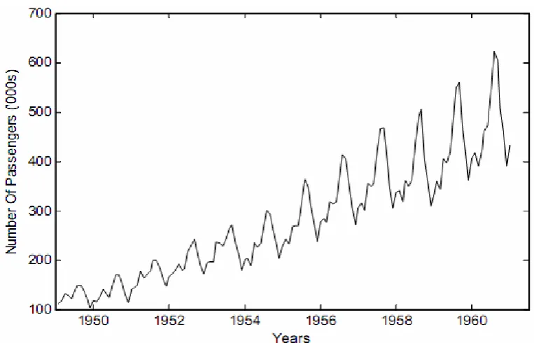
A time series is a sequential set of data points, measured typically over successive times. It is mathematically defined as a set of vectors x(t),t = 0,1,2,... where t represents the time elapsed. The variable x(t( is treated as a random variable. The measurements taken during an event in a time series are arranged in a proper chronological order a time series containing records of a single variable is termed as multivariate. But if records of more than one variable are considered, it is termed as multivariate. A time series can be continuous or discrete. In a continuous time series observations are measured at every instance of time, whereas a discrete time series contains observations measured at discrete points of time. For example temperature readings, flow of a river, concentration of a chemical process etc. can be recorded as a continuous time series. On the other hand population of a particular city, production of a company, exchange rates between two different currencies may represent discrete time series. Usually in a discrete time series the consecutive observations are recorded at equally spaced time intervals such as hourly, daily, weekly, monthly or yearly time separations in Figure 2.4, Figure 2.5. As mentioned in, the variable being observed in a discrete time series is assumed to be measured as a continuous variable using the real number scale. Furthermore a continuous time series can be easily transformed to a discrete one by merging data together over a

specified time interval.

Two different types of models are generally used for a time series viz. Multiplicative and Additive models.

Multiplicative Model: Y(t) =T(t)×S(t)×C(t)×I(t ) (2.16) Additive Model: Y(t) =T(t)+ S(t)+C(t)+ I(t) (2.17)

Here Y(t) is the observation and T(t) , S(t) , C(t) and I(t) are respectively the trend, seasonal, cyclical and irregular variation at time t.

(29)

[image:29.595.117.529.72.321.2]

19

Figure 2.4: Weekly BP/USD exchange rate series (1980-1993)

Figure 2.5: Monthly international airline passenger series (Jan. 1949-Dec. 1960)

2.5 Model validation methods

[image:29.595.118.500.370.615.2]

(30)

20

satisfy analysis objectives. Whereas model verification techniques are general the approach taken to model validation is likely to be much more specific to the model,

and system, in question. Indeed, just as model development will be influenced by the objectives of the performance study, so will model validation be. A model is usually developed to analyze a particular problem and may therefore represent different parts of the system at different levels of abstraction.

As a result, the model may have different levels of validity for different parts of the system across the full spectrum of system behavior. For most models there are three separate aspects which should be considered during model validation:

(i) Assumptions

(ii) input parameter values and distributions

(iii) Output values and conclusions.

However, in practice it may be difficult to achieve such a full validation of the model, especially if the system being modelled does not yet exist. In general, initial validation attempts will concentrate on the output of the model, and only if that validation suggests a problem will more detailed validation be undertaken. Broadly speaking there are three approaches to model validation and any combination of them may be applied as appropriate to the different aspects of a

particular model. These approaches are: (i) Expert intuition

(ii) Real system measurements (iii) Theoretical results/analysis.

In addition, as suggested above, ad hoc validation techniques may be established for a particular model and system [18].

2.5.1 Internal Validation

The most common internal method of validating the model is least squares fitting. This method of validation is similar to linear regression and is the (squared

(31)

21

activities. An improved method of determining is the robust straight line fit, where data points are away from the central data points (essentially data points a specified standard deviation away from the model) are given less weight when

calculating the . An alternative to this method is the removal of outliers (compounds from the training set) from the dataset in an attempt to optimize the QSAR model and is only valid if strict statistical rules are followed. The difference

between the value is less than 0.3 indicates that the number of descriptors involved in the QSAR model is acceptable. The number of descriptors is not acceptable if the difference is more than 0.3 [19].

=

{

∑ (∑ )(∑ )

√[( ∑ (∑ ) )][ ∑ (∑ ) ]

}

(2.18)

Where:

Dependent variable;

Independent variable;

Number of variable;

2.5.2 External validation

Several authors have suggested that the only way to estimate the true predictive

power of a QSAR model is to compare the predicted and observed activities of an sufficiently large external test set of compounds. The problem in external validation is how can we select the training and test set. clearly discussed that how we can solve this problem in one of their article22. To estimate the predictive power of a QSAR model, Golbraikh and Tropsha recommended use of the following statistical characteristics of the test set14: (i) correlation coefficient R between the predicted and observed activities; (ii) coefficients of determination predicted vs. observed

activities , and observed vs. predicted activities; (iii) slopes k and k' of the

(32)

22

Pred > 0.6,

- / < 0.1, r2 - / < 0.1 and

0.85 k 1.15 or 0.85 k’ 1.15 (2.19)

.

The predictive ability of the selected model was also confirmed by external pred. A value of pred is greater than 0.6 may be taken as an indicator of good external

predictability.

=1-∑ ( )

∑ ( )

(2.20)

Where

(33)

23

CHAPTER 3

METHODOLOGY

3.1 Power load data collection

(34)

[image:34.595.188.451.90.369.2]

24

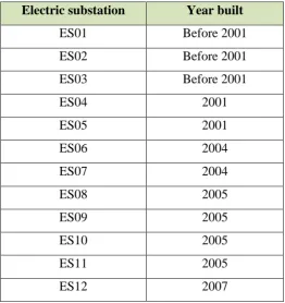
Table 3.1: Year of each electric substation was built

Electric substation Year built

ES01 Before 2001

ES02 Before 2001

ES03 Before 2001

ES04 2001

ES05 2001

ES06 2004

ES07 2004

ES08 2005

ES09 2005

ES10 2005

ES11 2005

ES12 2007

3.2 Analysis

The actual data as mentioned in section 3.1 is used to determine the future load demand of UTHM network. The work is performed using EXCEL software to derive an equation based on the existing data. EXCEL curve fitting tool known in the insert and layout has the ability to generate various types of equations such as Linear regressions and polynomial. The next step is to use MATLAB to derive an ANN approach by training the neurons in the specific layers. These layers consists of single input layer, one or more hidden layers and single output layer. The input layer contains of a number of neurons equals to the number of input variables in the training network by an iterative process. The weights are adjusted using some learning algorithms. For the purpose of forecasting in this project, two types of equations have been chosen linear regression and polynomial equations, ANN will be used in dynamic load forecasting after the static load forecasting is conducted.

(35)

56

REFERENCES

[1] D. W. Bunn and E. D. Farmer, ''Economic and Operation Context of Electric load prediction'', in D. W. Bunn and E. D. Farmer,

(ed.),Comparative models for Electrical load forecasting, pp.3-11, New

York: John Wiley and Sons Ltd., 1985.

[2] Andrew P. Douglas et al., ''Risk Due Load forecast Uncertainty in Short Term Power System Planning'', IEEE Transactions on Power System, Vol. 13, No. 4, PP. 1499, November 1998.

[3] Robert Fich1, ''Security Assessment and Enhancement, in Application Of Artificial Neural Network to Power System'', M. A. El-Sharkawy And Degmar Neural (eds.), pp. 104-127, New Jersey: The Institute of Electrical and Electronic Engineers, Inc., 1996

[4] S. Crary, “Steady state stability of composite systems,” Electrical Engineering, vol. 52, pp. 787–792, Nov. 1933.

[5] IEEE Task Force on Load Representation for Dynamic Performance, “Standard load models for power flow and dynamic performance

simulation,” IEEE Trans. Power Syst., vol. 10, no.3, pp. 1302–1313, Aug

1995.

(36)

57

[7] IEEE Task Force on Load Representation for Dynamic Performance, “Load representation for dynamic performance analysis (of power systems),”

IEEE Trans. Power Sys t., vol. 8, no. 2, pp. 472–82, May 1993.

[8] D. C. Montgomery, C. L. Jennings, M. Kulahci, Introduction to Time Series

Analysis and Forecasting, Publisher John Wiley and Sons, ISBN

978-0-471-65397-4.

[9] Introduction to Time Series Analysis

http://www.itl.nist.gov/div898/handbook/pmc/section4/p mc4.htm

[10] Ganesan, Rajesh, et al. "Regression and ANOVA: an integrated approach

using SAS software." IIE Transactions 36.12 (2004): 1211-1216.

[11] Inés, Romero Navarro. "Dynamic Load Models for Power

Systems-Estimation of Time-Varying Parameters During Normal Operation." TEIE 1034 (2002).

[12] Bunnoon, Pituk. "Mid-Term Load Forecasting Based on Neural Network Algorithm: a Comparison of Models."

[13] Park, Dong C., et al. "Electric load forecasting using an artificial neural network." Power Systems, IEEE Transactions on 6.2 (1991): 442-449.

[14] Ghods, Ladan, and Mohsen Kalantar. "Different Methods of Long-Term Electric Load Demand Forecasting; A Comprehensive Review." Iranian

Journal of Electrical & Electronic Engineering 7.4 (2011): 249.

[15] Yasar, Y. Aslan S. Yavasca C. "LONG TERM ELECTRIC PEAK LOAD FORECASTING OF KUTAHYA USING DIFFERENT APPROACHES.

(37)

58

[17] Zhang, Guoqiang, B. Eddy Patuwo, and Michael Y Hu. "Forecasting with artificial neural networks:: The state of the art." International journal of

forecasting 14.1 (1998): 35-62.

[18] Oreskes, Naomi, Kristin Shrader-Frechette, and Kenneth Belitz. "Verification, validation, and confirmation of numerical models in the earth sciences."Science 263.5147 (1994): 641-646.

[19] Veerasamy, Ravichandran, et al. "Validation of QSAR Models-Strategies

and Importance.

[20] Gavin, Henri. "The Levenberg-Marquardt method for nonlinear least squares curve-fitting problems." Department of Civil and Environmental

Engineering, Duke University (2011).

[21] M.I.A. Lourakis. A brief description of the Levenberg-Marquardt algorithm

implemented by levmar, Technical Report, Institute of Computer Science,

Foundation for Research and Technology- Hellas, 2005.

[22] K. Madsen, N.B. Nielsen, and O. Tingleff. Methods for nonlinear least

squares problems. Technical Report. Informatics and Mathematical

Dynamic load forecasting for commercial power network

TABLE OF CONTENTS

LIST OF TABLES

LIST OF FIGURES

LIST OF SYMBOLS AND ABBREVIATIONS

LIST OF APPENDICES

APPENDIX

TITLE

PAGE

.

+ … +

.

+

=



=





=





=

{

}