Georgia State University
ScholarWorks @ Georgia State University
Economics Dissertations Department of Economics
5-11-2015
Essays On Housing Tax Policy and Discrimination
in the Mortgage Market
William H. Martin Georgia State University
Follow this and additional works at:https://scholarworks.gsu.edu/econ_diss
This Dissertation is brought to you for free and open access by the Department of Economics at ScholarWorks @ Georgia State University. It has been accepted for inclusion in Economics Dissertations by an authorized administrator of ScholarWorks @ Georgia State University. For more information, please [email protected].
Recommended Citation
Martin, William H., "Essays On Housing Tax Policy and Discrimination in the Mortgage Market." Dissertation, Georgia State University, 2015.
ABSTRACT
ESSAYS ON HOUSING TAX POLICY AND DISCRIMINATION IN THE MORTGAGE MARKET
By
WILLIAM HAROLD MARTIN
March 2015
Committee Chair: Dr. Kurt Schnier
Major Department: Economics
This dissertation explores the impact of tax policy and institutions on decisions in the
market for housing. Two essays address the impact of tax policy on home values, neighborhood
accessibility, and public finance; a third essay presents an experimental test for discrimination in
mortgage lending.
The first essay is joint work with Andrew Hanson. In it, we estimate the sensitivity of
mortgage interest deducted on federal tax returns to the availability of the Mortgage Interest
Deduction (MID). Our primary results show that for every one percentage point increase in the
tax rate that applies to deductibility, the amount of mortgage interest deducted increases by
$303–590. We also compute the elasticity of mortgage interest and deadweight loss of the tax
policy.
The second essay simulates changes to average home prices in twenty-seven cities that
would result were the MID reformed. I use local variation in housing parameters to simulate
home price changes for three different reforms: eliminating the MID, converting the MID to a
fifteen percent credit, and capping the MID at fifteen percent. City price changes vary in
is also notable, with areas high in income experiencing steeper price declines and areas of lower
income experiencing shallow declines. To varying degrees, each reform reduces price
differences across neighborhoods, making more neighborhoods affordable to any given income
class.
The third essay is joint work with Andrew Hanson, Zack Hawley, and Bo Liu. We
design and implement an experimental test for differential response by Mortgage Loan
Originators (MLOs) to requests for information about loans. Our e-mail correspondence
experiment is designed to analyze differential treatment by client race and credit score. Our
results show net discrimination of 1.8 percent by MLOs through non-response. We also find that
MLOs offer more details about loans and are more likely to send follow up correspondence to
whites. The effect of being African American on MLO response is equivalent to the effect of
ESSAYS ON HOUSING TAX POLICY AND DISCRIMINATION IN THE MORTGAGE MARKET
BY
WILLIAM HAROLD MARTIN
A Dissertation Submitted in Partial Fulfillment of the Requirements for the Degree
of
Doctor of Philosophy in the
Andrew Young School of Policy Studies of
Georgia State University
Copyright by William Harold Martin
ACCEPTANCE
This dissertation was prepared under the direction of the candidate’s Dissertation
Committee. It has been approved and accepted by all members of that committee, and it has been accepted in partial fulfillment of the requirements for the degree of Doctor of Philosophy in Economics in the Andrew Young School of Policy Studies of Georgia State University.
Dissertation Chair: Dr. Kurt Schnier
Committee: Dr. Spencer Banzhaf Dr. Andrew Hanson Dr. Sally Wallace
Electronic Version Approved:
Mary Beth Walker, Dean
Andrew Young School of Policy Studies Georgia State University
iv
ACKNOWLEDGEMENTS
It takes a community to raise a scholar. I am grateful to the community at the Andrew
Young School for all it has done to develop its students into well-rounded researchers. My
committee exemplifies the range of talents and qualities that served me well as I advanced
through my academic career.
Andrew Hanson became my mentor early on, and despite changing institutions has
remained my closest collaborator. I value his guidance and training in how to think about
research questions, how to talk about them in published work, and how to approach life as an
academic economist. I am also grateful to Kurt Schnier for his advice and support, particularly
through the middle of my graduate studies as I sorted out the type of research that I want to do.
Spencer Banzhaf is a bastion of microeconomic analysis, and I am grateful for his relentless
example of using economic theory to evaluate and interpret empirical findings in order to
sharpen one’s work. I am grateful to Sally Wallace for asking incisive questions that improve
how I approach my work and for teaching me the value of being familiar with as broad an array
of data resources as possible.
My graduate studies were also facilitated by a well-functioning administration, which
cannot be overpraised. Bess Blyler and her colleagues who support the administrative functions
of the department do so much to make our academic lives run smoothly, for which they deserve
many thanks.
Finally, I am grateful to my wife Amanda for her steadfastness and patience as I pursued
the peculiar activity of acquiring a doctorate in Economics. And to Zippy and Zora, for putting
the challenges I faced in graduate school into perspective with a refreshing walk outside, or
v
TABLE OF CONTENTS
ACKNOWLEDGEMENTS ... iv
List of Tables ... vii
List of Figures ... ix
Abbreviations ... x
Introduction ... 1
Chapter I Housing Market Distortions and the Mortgage Interest Deduction ... 4
1. Introduction ... 4
2. Background and Related Literature ... 6
3. Identification Strategy for Elasticity Estimates ... 8
4. Data ... 14
5. Estimation Results, Elasticities, and Deadweight Loss ... 16
6. Conclusion ... 30
Chapter II The Impact of Housing Tax Preferences on Home Values and Neighborhood Sorting ... 32
1. Introduction ... 32
2. Background and Related Literature ... 34
3. Model Design ... 37
4. Data ... 42
5. Model Adjustments to Simulate Policy Changes ... 45
6. Identification Strategy for Model Parameters ... 48
7. Results ... 54
8. Conclusion ... 75
Chapter III Discrimination in Mortgage Lending: Evidence from a Correspondence Experiment ... 77
1. Introduction ... 77
2. MLOs in the Lending Process ... 81
3. Experiment Design ... 82
4. Experiment Implementation and Sample Characteristics ... 89
5. Results ... 94
vi
7. Conclusion ... 115
Appendix 1. Correspondence Construction ... 117
Appendix 2. Side-by-Side Comparison Tool ... 118
Appendix 3. Grader Instructions for Side-by-Side Comparison ... 119
Conclusion ... 120
References ... 123
vii
List of Tables
Table 1. First Stage Instrumental Variable Results ... 13
Table 2. Summary Statistics ... 15
Table 3. Effect of Mortgage Interest Deductibility on Annual Mortgage Interest Claimed ... 17
Table 4. Effect of Mortgage Interest Deductibility on Annual Mortgage Interest Claimed (Including HVI) ... 19
Table 5. Elasticity of Mortgage Interest Deductibility with Respect to Tax Induced User Cost Change ... 23
Table 6. Deadweight Loss from the Mortgage Interest Deduction ... 26
Table 7. Tax Revenue Estimates for MID Policy Changes ... 28
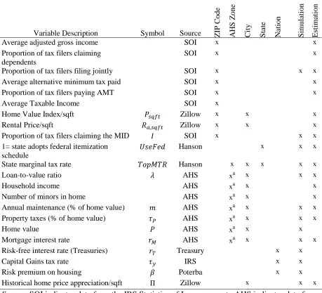
Table 8. Description of Variables ... 43
Table 9. First Stage Results of Instrumental Variables Specification ... 51
Table 10. Impact of the Mortgage Interest Deduction on the Percent of Itemizing Tax Filers .... 55
Table 11. Impact of the MID on the Loan-To-Value (LTV) Ratio of Homeowners ... 56
Table 12. WLS Tests of User Cost Parameters... 57
Table 13. Behavioral Parameter Changes Resulting from MID Policy Changes ... 59
Table 14. Percent Change in User Cost Resulting from MID Policy Changes ... 60
Table 15. Simulated Effects on Home Prices of Policy Changes to the Mortgage Interest Deduction ... 62
Table 16. Percent Change in Housing Expenditure Required for Upward Mobility within a City ... 73
Table 17. Names Identifying Race... 87
viii
Table 19. Number of Audits and Response Rate across States ... 90
Table 20. Mortgage Loan Originator Characteristics ... 92
Table 21. Response Rate and Mortgage Loan Originator (MLO) Level Response to Race
Differences ... 96
Table 22. Response Rate and Mortgage Loan Originator (MLO) Level Response to Credit Score
Differences ... 99
Table 23. Response Rate and Mortgage Loan Originator (MLO) Level Response by Race and
Credit of Credit-Seeker ... 101
Table 24. Intensity of Mortgage Loan Originator (MLO) Response ... 104
Table 25. Side-by-Side Comparison of Mortgage Loan Originator(MLO) Response Content .. 107
Table 26. Name Robustness and National Popularity ... 112
ix
List of Figures
Figure 1. State Tax Policy Regarding the Mortgage Interest Deduction ... 9
Figure 2. Eliminating the MID in Atlanta, GA ... 66
Figure 3. Converting the MID to a 15% Credit in Atlanta, GA... 66
Figure 4. Capping the MID at 15% in Atlanta, GA ... 67
Figure 5. Eliminating the MID in Los Angeles, CA ... 68
Figure 6. Converting the MID to a 15% Credit in Los Angeles, CA ... 68
Figure 7. Capping the MID at 15% in Los Angeles, CA ... 69
Figure 8. Eliminating the MID in Pittsburgh, PA ... 70
Figure 9. Converting the MID to a 15% Credit in Pittsburgh, PA... 70
Figure 10. Capping the MID at 15% in Pittsburgh, PA ... 71
x
Abbreviations
AA African American
AGI adjusted gross income
AHS American Housing Survey
AMT alternative minimum tax
DHHH Department of Health and Human Hygiene
DOJ Department of Justice
EDT Eastern Daylight Time
HMDA Home Mortgage Disclosure Act
HVI home value index
IV instrumental variables
LTV loan to value
MID mortgage interest deduction
MLO mortgage loan officer
MSA metropolitan statistical area
MTR marginal tax rate
NMLS Nationwide Mortgage Licensing System
SAFE Secure and Fair Enforcement for Mortgage Licensing Act
SMTP Simple Mail Transfer Protocol
SOI Statistics of Income (division of IRS)
TRA86 Tax Reform Act of 1986
1
Introduction
Housing is among the largest markets in which consumers participate. It is also heavily
influenced by a variety of public policies and institutions. In this dissertation I explore the
impact of a specific tax policy, the Mortgage Interest Deduction (MID), on different aspects of
the housing market. I also explore the role that racial discrimination plays in access to mortgage
lending. A recurring theme throughout the dissertation is an examination of the heterogeneous
effects of policies and institutions on different social groups, including income class and race.
The first essay is joint work with Andrew Hanson. We use data on federal tax returns to
estimate the sensitivity of mortgage interest deducted to the availability of the MID. Our
primary results show that for every one percentage point increase in the tax rate that applies to
deductibility, the amount of mortgage interest deducted increases by $303–590. This work
complements a variety of studies1 that examine different margins on which the MID affects
consumer behavior by capturing the joint effect of those decisions through mortgage interest
payments as reported in tax returns. We also compute the elasticity of mortgage interest and
deadweight loss of the tax policy. Finally, we calculate the change in tax expenditure by income
class for each alternative policy that we consider. The tax expenditure of the MID is highest for
middle and upper-middle income classes. The high elasticity estimates we find suggest that
behavioral response to MID reform would substantially reduce the tax revenue generated from
MID reform compared with static estimates, which is consistent with observations by Poterba
and Sinai (2011).
2
In the second essay I combine data on federal tax returns with local household data from
the American Housing Survey to simulate the impact of MID reform on average home prices in
twenty-seven cities.2 I employ the user cost model to simulate home price changes at both the
city and neighborhood levels for three different reforms: eliminating the MID, converting the
MID to a fifteen percent credit, and capping the MID at fifteen percent. I also propose
improvements to the user cost model by calibrating key parameters that are often taken on
assumption in the existing literature. I find that price effects vary substantially across cities; for
instance, eliminating the MID would decrease prices by as much as 15.7 percent in Washington,
D.C. and by as little as 3.2 percent in Memphis. There is also substantial variation between
neighborhoods that closely correlates to income levels. I find suggestive evidence that the MID
reinforces income class barriers between neighborhoods, and I estimate that the affordability gap
between neighborhood income quartiles decreases by as much as 17.7 percent under MID
reform.
The third essay is joint work with Andrew Hanson, Zack Hawley, and Bo Liu. We
design and implement an experimental test for differential response by Mortgage Loan
Originators (MLOs) to requests for information about loans. Using an email audit technique, we
test whether mortgage loan officers discriminate against potential clients on the basis of race.
We find a net difference in response rate of 1.8 percent favoring whites. A subset of our subjects
are exposed to stated credit scores, allowing us to compare racial discrimination to credit
discrimination. We find that the response rate differential of being African American is
equivalent to having a lower credit score by 71 points. We also find that MLOs offer more
details about loans and are more likely to send follow up correspondence to whites.
3
On the whole, this work provides evidence of the heterogeneous effects of policy and
institutions in the housing market. The first essay shows how consumer behavior and tax policy
interact to produce an uneven distribution of benefits across income classes and distortions in the
housing market. The second describes the uneven distribution of the MID across space, owing to
differences in home prices, take-up rates through itemization and marginal tax rates. The third
4
Chapter I
Housing Market Distortions and the Mortgage Interest Deduction3
1. Introduction
The largest government intervention in housing markets is the mortgage interest
deduction (MID). The Executive Office of the President (2011) estimates that the MID amounts
to $98.5 billion in foregone revenues in 2012, and $609 billion between 2012 and 2016. There is
a large and growing literature suggesting that the MID distorts housing market decisions, mainly
by increasing the demand for mortgage debt in favor of equity financing (Jones 1995; Ling and
McGill 1998; Dunsky and Follain 2000; Hendershott and Pryce 2006; Poterba and Sinai 2011),
or increasing the size of home (Hanson 2012b). 4 The MID may also distort decisions by
inducing renters to become owners, incentivizing the purchase of a second home, purchasing a
larger lot, choosing a longer term mortgage, changing the speed that debt is paid off, and
inducing those who would otherwise claim the standard deduction to itemize their tax deductions
(or to increase other itemized deductions). The existing body of work on the distortions caused
by the MID may not be sufficient to measure the full deadweight loss from the subsidy because it
does not jointly capture all of these distortions.
To capture the full distortion caused by the MID, we measure how sensitive mortgage
interest deduction claims are to the interaction between MID availability and marginal tax rates.
This is analogous to Feldstein (1995; 1999) relating the full distortion from of the income tax to
the sensitivity of taxable income, rather than a more narrow measure like hours worked or labor
3 This essay is based on joint work with Andrew Hanson of Marquette University.
5
force participation. We relate the distortion from the MID to the sensitivity of mortgage interest
deducted to capture the full distortionary effect of the deduction, rather than a more narrow
measure like home size or self-reported levels of housing debt. While we consider many of these
more narrow measures interesting in their own right,5 a more comprehensive measure is
necessary to accurately portray deadweight loss from the MID.6
Using Internal Revenue Service ZIP code level data, we first estimate the sensitivity of
MID claims to state level variation in top marginal income tax rates and availability of the MID.
In addition to weighted least squares, we use several comparison groups to estimate this
relationship, as well as estimating with instrumental variables. Our primary results show that for
every one percentage point increase in the top marginal tax rate, the amount of mortgage interest
deducted increases by $303–590. We then combine the empirical estimates with the user cost
model of housing to produce elasticities of mortgage interest deducted with respect to the
after-tax cost of housing – these estimates range from -0.78 to -1.862. With these elasticities in hand
we estimate the total amount of deadweight loss caused by the MID to be between 16 and 36
percent of the tax expenditure. We also use our elasticity estimates to consider how sensitive
federal revenues are to changes in MID policy, including switching the deduction to a credit or
eliminating it entirely.
The remainder of the paper begins by briefly discussing the existing literature on MID
induced distortions. Section 3 discusses our identification strategy for empirically estimating the
sensitivity of mortgage interest deductions to availability and generosity of the deduction.
5 For example, from a policy perspective it is important to know if the MID is inducing home ownership, as this may aid in bringing home ownership rates to the socially optimal level if there are externalities from ownership.
6
Section 4 details the data we use in estimation, and Section 5 discusses our main empirical
results and how they relate to elasticity, deadweight loss, and tax revenue estimates. The final
section of the paper concludes.
2. Background and Related Literature
The literature examining distortions from the mortgage interest deduction prior to 1990
primarily focused on how deductibility alters the debt-financing decision of home purchasers.
Smith, Rosen and Fallis (1988) summarize this literature and describe the primary distortion
from the tax treatment of housing to be a substantial increase in homeownership rates, by as
much as 4 percentage points. The literature up to that time focused on identifying the
relationship between ownership and generosity of the mortgage interest deduction using
time-series variation in the U.S. homeownership rate. Later work, that shows no relationship between
ownership rates and generosity of the MID, uses both time series and cross section variation
(Glaeser and Shapiro 2003; Hanson 2012b).
Beginning in the mid-1990s, the literature shifted focus to examine distortions from the
MID in the home finance decision. Jones (1995), using Canadian data, finds a significant effect
of marginal tax rates on the amount of mortgage debt in a household’s portfolio. Ling and
McGill (1998) use 1985 and 1989 American Housing Survey data to estimate the effect of a
variety of factors on mortgage debt, including income tax rates. They find that mortgage debt is
highly sensitive to the potential tax savings it offers. Dunsky and Follain (1997; 2000) examine
the impact of the Tax Reform Act of 1986 (TRA86) on the demand for mortgage debt using data
from the Survey of Consumer Finances. TRA86 made tax savings on mortgage interest generally
smaller by lowering marginal rates and increasing the standard deduction. Dunsky and Follain
7
Hendershott and Pryce (2006) estimate the sensitivity of mortgage debt to changes in the
limits of deductibility, using data from the United Kingdom. They also estimate tax revenue
changes that would occur in response to changes in deductibility policy. They then simulate the
response of mortgage debt and tax revenue to the policy change of altogether removing the UK
MID. Using multiple specifications on multiple age brackets and across two regions they find
declines in the loan-to-value ratios in response to a shift from full MID to no MID that range
from 6.7 percent to 50.7 percent.
Poterba and Sinai (2008; 2011) consider the tax expenditure implications of property tax
and mortgage interest deductions. They estimate elasticities of mortgage debt with respect to the
after-tax interest rate to average -0.715 (they include several different estimates across income
groups). They model the way households might respond to an elimination of the MID and
conclude that revenue from such a policy change would be $72.4 billion if households do not
rebalance their portfolio in the face of tax adjustments and $58.5 billion if households do
rebalance their asset portfolios.
We extend the literature on the distortionary effects of the MID by offering a
comprehensive measure of the response to changes in policy generosity by examining the effect
on dollars deducted. This measure captures the full distortion potential of the MID by
encompassing all decisions that it may affect including: inducing renters to become owners,
incentivizing the purchase of a second home, purchasing a larger lot, choosing a longer term
mortgage, changing the speed that debt is paid off, and inducing those who would otherwise
claim the standard deduction to itemize deductions (or increase other itemized deductions). In
self-8
reported, as tax returns carry penalties and the threat of audit when information is given
inaccurately.
3. Identification Strategy for Elasticity Estimates
We use two primary techniques to identify the effect of the mortgage interest deduction
on the amount of mortgage interest that tax filers deduct: weighted least squares (WLS) and
instrumental variables (IV).7 Both identification strategies use variation in state MID policy
combined with state marginal tax rate differences to identify the effects of the MID on interest
deducted. While the federal MID is available to all income taxpayers who itemize deductions,
not all states have an income tax and not all states that have an income tax allow an MID.
Following (Hanson 2012b), the WLS estimates use a variety of comparison groups to
identify the effect of the MID on dollars of mortgage interest deducted including: all states, only
other income tax states, and only states with a top marginal income tax above the median.
Figure 1 shows the variation in MID policy we use to categorize states into groups. As the figure
shows, there are several states that choose not to allow an MID, while several others do not have
an income tax and therefore do not allow an MID. The WLS estimation may be biased if states
choose MID policy endogenously – that is, if tax filers with large amounts of mortgage interest
cause states to adopt an MID. IV estimation mitigates this concern by instrumenting for state
MID policy using adoption of all federal itemized deductions to explain the existence of a state
level MID.
9
Figure 1. State Tax Policy Regarding the Mortgage Interest Deduction
3.1 Weighted Least Squares
We use weighted least squares, rather than ordinary least squares, as our primary
estimation technique to ensure our regressions are representative of the population of tax filers.
Our data are at the ZIP code level (see data section for complete description), and since ZIP
codes contain uneven numbers of tax filers we weight the regressions to get an appropriate
estimate. We weight our regression using the square root of the number of MID claims in each
ZIP code and estimate the effect of the MID on the dollars of mortgage interest deducted with
the following regression:
𝐷𝑜𝑙𝑙𝑎𝑟𝑠 𝐷𝑒𝑑𝑢𝑐𝑡𝑒𝑑𝑖 = 𝛼 + β1𝑇𝑜𝑝𝑀𝑇𝑅𝑖 ∗ 𝑀𝐼𝐷𝑖 + 𝐙𝒊′+ 𝜀 (1)
Figure 1: State MID and Income Tax Policy
MID not allowed
MID allowed
10
where 𝐷𝑜𝑙𝑙𝑎𝑟𝑠 𝐷𝑒𝑑𝑢𝑐𝑡𝑒𝑑 is the average amount of mortgage interest deducted per MID claim
for each ZIP code, 𝑇𝑜𝑝𝑀𝑇𝑅 is the top marginal tax rate in the state, 𝑀𝐼𝐷 is an indicator variable
equal to one if the state allows the MID and zero if it does not.8𝒁 is a set of control variables that
includes the average adjusted gross income (AGI) of tax filers, the proportion of tax filers
claiming dependents, the proportion of tax filers completing a joint return, the average amount of
all other itemized deductions per tax filer (and the square of this term), the proportion of filers
subject to the alternative minimum tax, and the average dollar amount of alternative minimum
tax (AMT) paid per AMT filer.9 We correct all standard error estimates in equation 1 for
heteroskedasticity using the White (1980) correction following the explanation in (Winship and
Radbill 1994), to account for the effects of the weighting procedure on standard errors.
Using equation 1 to estimate the effect of the MID on the dollars of mortgage interest
deducted relies on three primary assumptions. First, tax filers in states without an MID make a
valid counter-factual for what tax filers in states with an MID would deduct in the absence of the
state level MID. Second, there are no omitted variables influencing the amount of mortgage
interest deducted that are correlated with availability of the MID. Third, the MID is not
endogenous – individuals with larger deductions do not cause states to have an MID.
Controlling for observed factors alleviates some concerns about omitted variables. Supposing
unobservables might be correlated with income tax rates, we attempt to alleviate this concern by
using alternative comparison groups of states with similar state income tax rates. We use two
alternative comparison groups: states without an MID but that have an income tax, and states
8 (Hanson 2012b) explains the benefits of using a proxy for an individual’s marginal tax rate, rather than the actual marginal tax rate, which is likely endogenous. This explanation is based on the argument in (Angrist and Pischke 2009) that proxies can reduce bias in estimation.
11
without an MID but with a top marginal income tax rate higher than the median states of
Georgia, Kentucky, Louisiana and Missouri (each with a top marginal income tax rate of 6.00
percent).
3.2 Instrumental Variables
Using alternative comparison groups may eliminate some of the unobservable differences
between states that allow an MID and states that do not; however, it is still possible that
unobservables exist and are correlated with MID policy. It is also possible that classic
endogeneity is still present – residents with high amounts of mortgage debt lobby states to enact
mortgage interest deductions. As a further guard against the possibility that omitted variables or
reverse causality are a problem in equation 1, we estimate an IV specification.
Our instrument for state level MID availability follows (Hanson 2012b), and is an
indicator variable of whether a state follows the federal definition of itemized deductions. An
instrument in this case requires a variable correlated with a state allowing a deduction for
mortgage interest, but only correlated with home size through its correlation with state MID
policy. A state’s adoption of the federal definition of itemized deductions is arguably
uncorrelated with many of the potential sources of omitted variable bias and reverse causality
between the MID and home size because it implies that the residents of the state did not actively
lobby to get a MID. States that take the federal definition of itemized deductions allow all
federal deductions, not just the MID, so it is unlikely that having this policy is strongly correlated
with resident preferences for housing consumption. States still actively choose to allow the
federal definition of itemized deductions, but this would most likely be the result of influence
12
including for medical and dental expenses, state and local taxes, gifts to charity, and business
expenses incurred.
Our first stage for the instrumental variables regressions is:
𝑀𝐼𝐷𝑖 = 𝛼 + β1𝐹𝑒𝑑𝐼𝑡𝑒𝑚𝑖 + 𝐙𝒊′∗ +𝜀 (2)
where 𝐹𝑒𝑑𝐼𝑡𝑒𝑚 is a dummy variable equal to one if a state follows the federal definition of
itemized deductions, and zero otherwise, and 𝒁 is the same set of control variables from equation
1. We obtain the predicted values of 𝑀𝐼𝐷𝑖 for each ZIP code and use them in the second stage
regression weighted by the number of tax filers in each ZIP code:
𝐷𝑜𝑙𝑙𝑎𝑟𝑠 𝐷𝑒𝑑𝑢𝑐𝑡𝑒𝑑𝑖 = 𝛼 + β1𝑀𝐼𝐷̂ ∗ 𝑇𝑜𝑝𝑀𝑇𝑅𝑖 𝑖 + 𝐙𝒊′+ 𝜀 (3)
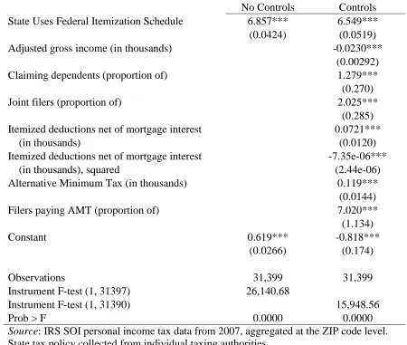
Table 1 shows the first stage IV results. These results show a strong correlation between
states that follow the federal definition of itemization and allowing a state level MID. In both the
specification with control variables and without them, the F-statistic is well above the customary
10 that suggests instrument validity, showing that the correlation between the instrument and the
13 Table 1. First Stage Instrumental Variable Results
No Controls Controls State Uses Federal Itemization Schedule 6.857*** 6.549***
(0.0424) (0.0519)
Adjusted gross income (in thousands) -0.0230***
(0.00292)
Claiming dependents (proportion of) 1.279***
(0.270)
Joint filers (proportion of) 2.025***
(0.285)
Itemized deductions net of mortgage interest 0.0721***
(in thousands) (0.0120)
Itemized deductions net of mortgage interest -7.35e-06***
(in thousands), squared (2.44e-06)
Alternative Minimum Tax (in thousands) 0.119***
(0.0144)
Filers paying AMT (proportion of) 7.020***
(1.134)
Constant 0.619*** -0.818***
(0.0266) (0.174)
Observations 31,399 31,399
Instrument F-test (1, 31397) 26,140.68
Instrument F-test (1, 31390) 15,948.56
Prob > F 0.0000 0.0000
Source: IRS SOI personal income tax data from 2007, aggregated at the ZIP code level. State tax policy collected from individual taxing authorities.
14
4. Data
We use Internal Revenue Service (IRS) data on the universe of tax filers for 2007 to
estimate equations 1 – 6. The unit of observation in the IRS data is the ZIP code, broken into
seven classes of AGI. For our primary analysis we combine the data across seven classes into
one observation per ZIP code (revenue estimates make use of the individual AGI classes). The
data is limited in several ways. To protect taxpayer privacy, AGI classes with fewer than 10
observations are combined with the next lowest class.10 Taxpayers whose income forms an
undisclosed percentage of a ZIP code total are excluded entirely from the data. Also, the IRS
uses the self-reported ZIP code of each taxpayer and does not make any attempt to correct
invalid ZIP codes or impute missing ZIP codes. We view these limitations as minor, given the
detail they provide about MID claims across geography.
The data include counts of taxpayers who claim the MID as well as the total amount of
mortgage interest deducted for all ZIP codes in the U.S. – from this we form the dependent
variable, average MID claimed per return. The IRS data contain other relevant information
about dollar amounts and number of filers which we use to construct several control variables
including: average adjusted gross income of tax filers, the proportion of tax filers claiming
dependents, the proportion of tax filers completing a joint return, the average amount of all other
itemized deductions per itemizer, the proportion of filers subject to the alternative minimum tax,
and the average dollar amount of alternative minimum tax paid per AMT filer.
15
Although our data is only for one year of tax returns, we believe the advantages that it
offers in terms of the micro-level of geography and the detail on both MID claims and dollars
claimed are sufficient counter-weight to concerns about external validity across tax years.
Indeed, subsequent releases of the IRS ZIP code file do not include as detailed of information
about MID claims.11 Furthermore, the MID claimed in any given tax year is not the result of
decisions made in that year alone – it is instead the product of many preceding years of decisions
to contract for mortgage debt, with recent years weighted more heavily in the total due to the
amortization schedules used in home loans.
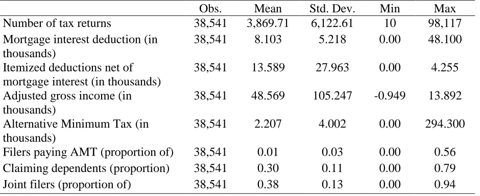
Table 2 provides summary statistics for the relevant variables we construct from the IRS
tax return data. The mean value of mortgage interest deduction is the mean of all ZIP code
[image:28.612.75.545.419.611.2]means, at $8,103. Itemized deductions, AGI, and AMT are also means of the ZIP code means.
Table 2. Summary Statistics
Obs. Mean Std. Dev. Min Max
Number of tax returns 38,541 3,869.71 6,122.61 10 98,117
Mortgage interest deduction (in thousands)
38,541 8.103 5.218 0.00 48.100
Itemized deductions net of mortgage interest (in thousands)
38,541 13.589 27.963 0.00 4.255
Adjusted gross income (in thousands)
38,541 48.569 105.247 -0.949 13.892
Alternative Minimum Tax (in thousands)
38,541 2.207 4.002 0.00 294.300
Filers paying AMT (proportion of) 38,541 0.01 0.03 0.00 0.56 Claiming dependents (proportion) 38,541 0.30 0.11 0.00 0.79
Joint filers (proportion of) 38,541 0.38 0.13 0.00 0.94
Source: IRS SOI personal income tax data from 2007, aggregated at the ZIP code level.
11 While the IRS provides data for prior years up through 2008, prior year data does not break out the MID from itemized deductions; 2008 data provides MID amounts by ZIP code, but not number of claims, making the
16
We combine the IRS data with state MID policy and top marginal tax rates using author
assembled data from state tax forms for tax year 2007. Two zip codes are listed in multiple
states, which is a data anomaly. Because we exploit state policy variation, we categorically
exclude all returns in the two ZIP codes that erroneously cross state borders.
5. Estimation Results, Elasticities, and Deadweight Loss
Table 3 shows estimation results for equations 1 and 3. These results show that the
generosity of the mortgage interest deduction (as measured by the interaction between MID
availability and state top marginal tax rate) is positively correlated with the amount of mortgage
interest tax filers deduct. The WLS results, shown in columns 1 – 6, suggest that for every
percentage point increase in the top marginal tax rate, tax filers deduct an additional $303-590 of
mortgage interest. The magnitude of the coefficient of interest depends on the comparison group
we use, with smaller magnitudes when the comparison group is “all other” states, and larger
magnitudes when the comparison group is only states with an income tax rate above the median.
The magnitude is slightly larger for specifications without control variables, and is statistically
17
Table 3. Effect of Mortgage Interest Deductibility on Annual Mortgage Interest Claimed
All Observations State Income Tax > 0
State Income Tax >
median IV: All Observations No
Controls Controls
No
Controls Controls
No
Controls Controls
No
Controls Controls Top marginal tax ratea * (state 388.8*** 340.2*** 493.5*** 455.0*** 589.9*** 574.6*** 376.2*** 303.0*** mortgage interest deduction
allowed = 1)
(13.81) (12.01) (15.24) (11.53) (20.51) (15.14) (13.59) (11.54)
Adjusted gross income (in thousands) 41.19*** 28.02*** -0.637 38.21***
(4.450) (4.437) (3.226) (4.098)
Claiming dependents (proportion of) 5,851*** 7,441*** 9,431*** 6,054***
(508.8) (562.0) (680.6) (501.2)
Joint filers (proportion of) -3,023*** -2,761*** -4,995*** -2,710***
(450.7) (478.6) (572.1) (438.1)
Itemized deductions net of mortgage -95.20*** -49.42*** 33.89** -91.77***
interest (in thousands) (17.84) (17.98) (16.48) (15.93)
Itemized deductions net of mortgage -0.0110 -0.0103 -0.0109** -0.0112
interest (in thousands), squared (0.0105) (0.00768) (0.00509) (0.0107)
Alternative Minimum Tax (in 174.9*** 65.24** 57.29* 229.9***
thousands) (36.13) (26.97) (32.75) (21.86)
Filers paying AMT (proportion of) 42,141*** 51,638*** 64,786*** 42,432***
(2,621) (2,454) (2,165) (2,552)
Observations 32,779 32,779 27,289 27,289 18,062 18,062 31,399 31,399
R squared 0.108 0.532 0.148 0.593 0.157 0.591
Source: IRS SOI personal income tax data from 2007, aggregated at the ZIP code level. State tax policy collected from individual taxing authorities.
atax rate given in percent terms, i.e. 5.00 percent given as 5.00
18
We also estimate each sample in WLS and IV using an alternate set of controls that
includes a local home value index. We use the average monthly ZIP code level home value
index (HVI) for 2007 constructed by Zillow, a private firm that collects and uses real estate data.
Adding this control departs fundamentally from our general equilibrium framework – whereas
our other estimates permit the impact of the MID on all dimensions of the market (including
home values) to be captured in the subsidy, the set of specifications that include HVI as a control
breaks out one of the dimensions on which the MID presumably distorts markets.
Table 4 reports the results of regressions that control for local home prices. The
coefficient of interest is now considerably lower, ranging from $96-240 for a one percent
increase in the MID subsidy. The effect is muted by the coefficient on the HVI, which ranges
from $24-26. This implies a linear change of one point in the HVI index leads to an increase of
$24-26 in mortgage debt.
These estimates reflect the impact of higher home values on a household’s decision to
incur a dollar of mortgage interest in a separate coefficient from the one we focus on up to this
point. An argument can be made that controlling for home values improves counterfactual
balance; however, home values are functionally related to the amount of mortgage debt a person
carries. Because of this, the meaning of the coefficient of interest is changed in these
specifications – it no longer measures total response to the tax subsidy, but the response net of
housing value change. We prefer not to break apart mortgage debt response into some of its
constituent components since our data does not allow an exhaustive breakdown to clearly
interpret the separate coefficients. Therefore our estimates going forward will not carry this
alternate set of controls. Given estimated coefficients roughly one-third of our preferred
19
Table 4. Effect of Mortgage Interest Deductibility on Annual Mortgage Interest Claimed (Including HVI) All Observations State Income Tax > 0 State Income Tax > median IV: All Observations Top marginal tax ratea * (state 96.75*** 209.0*** 240.2*** 96.13***
mortgage interest deduction allowed = 1)
(12.48) (12.72) (15.61) (10.71)
Adjusted gross income (in 39.43*** 36.42*** 11.19** 40.06***
thousands) (4.668) (3.563) (5.054) (4.456)
Claiming dependents (proportion of) 11,719*** 12,112*** 12,718*** 11,888***
(551.0) (516.6) (626.3) (499.3)
Joint filers (proportion of) 6,370*** 6,192*** 5,965*** 6,333***
(496.6) (470.3) (640.9) (483.9)
Itemized deductions net of mortgage -52.36*** -6.680 50.83*** -67.65*** interest (in thousands) (19.80) (17.72) (18.91) (16.63) Itemized deductions net of mortgage -0.219 -0.436*** -0.301*** -0.205 interest (in thousands), squared (0.149) (0.0911) (0.0704) (0.146)
Alternative Minimum Tax (in 156.0*** 44.58 30.95 225.4***
thousands) (51.83) (29.09) (29.23) (26.28)
Filers paying AMT (proportion of) 813.8 5,705** 15,922*** 1,079
(3,251) (2,798) (3,459) (3,194)
Zillow Home Value Index (per sqft) 26.44*** 24.62*** 24.37*** 26.20***
(0.817) (0.832) (0.899) (0.777)
Observations 9,456 7,837 5,231 9,283
R squared 0.790 0.827 0.828
Source: IRS SOI personal income tax data from 2007, aggregated at the ZIP code level. State tax policy collected from individual taxing authorities.
atax rate given in percent terms, i.e. 5.00 percent given as 5.00
20 Elasticity Estimates
The WLS and IV coefficients provide quantity change estimates- how sensitive the
amount of mortgage interest deducted is to a more generous MID. Elasticity estimates require
combining quantity change estimates with price change estimates. To calculate price change
estimates that are compatible with the quantity change estimates in table 3, we apply the user
cost model of housing to a one percent change in the top marginal tax rate. The user cost model
relates how a change in the tax rate that applies to the MID effects the annual cost of purchasing
housing. There is a long literature that relates the tax treatment of owner occupied housing to the
annual cost with the user cost model. See Rosen (1979a; 1979b; 1985), Poterba (1984; 1992),
Green and Vandell (1999a), Glaeser and Shapiro (2003), Himmelberg, Mayer and Sinai (2005),
Anderson, Clemens, and Hanson (2007), and Poterba and Sinai (2008, 2011) as examples.
We use the most recent version of the user cost model, presented in (Poterba and Sinai
2011), as it includes several innovations from previous iterations. Poterba and Sinai consider a
housing specific risk premium as a cost to borrowers, while recognizing that buyers benefit from
the reduction in risk associated with being able to pre-pay or default. Thus, the model excludes
the mortgage interest rate in excess of the risk free rate as a cost. With these considerations, and
current tax treatment, the user cost of housing with preferential tax treatment of mortgage
interest is:
𝑈𝐶 = (1 − {τ𝐷𝜆 + τ𝑌(1 − 𝜆)})𝑟𝑇+ (1 − τ𝑌)𝛽 − τ𝐷𝜆(𝑟𝑀− 𝑟𝑇) + 𝑚
+(1 − τ𝐷− 𝑘)τ𝑃− 𝜋 (4)
where τ𝐷 represents the marginal income tax rate applying to deductions, 𝜆 is the loan to value
21
interest rate, 𝛽 is a housing specific risk premium, and 𝑟𝑀 represents the mortgage interest rate.12
𝑚 is annual maintenance and depreciation costs, and τ𝑃 is the local property tax rate. The
parameter 𝑘, also an innovation to the user cost model added by Poterba and Sinai (2011), allows
flexibility in viewing the property tax as a benefit tax or an excise tax. If the property tax is
completely a benefit tax, then 𝑘 = 1, and we are left with only the deduction portion; if 𝑘 = 0,
then the property tax is completely an excise tax and the full cost (minus deduction) is included;
we assume that 𝑘 = 0. 𝜋 is expected annual home price inflation.
The parameters we use to estimate the user cost change from a one percentage point
increase in the marginal tax rate mostly follow(Poterba and Sinai 2011). We construct a
sample-specific marginal income tax rate composed of an average of state marginal tax rates in each
sample (weighted by the number of MID claims in each state) and a federal marginal tax rate of
25 percent. The weighted average state marginal tax rate ranges from 5.6 to 8.2 percent (the
former belonging to all observations and the latter to the sample of states with a tax rate greater
than the median of 6 percent). This results in an assumed 𝜏𝐷 ranging from 30.6 to 33.2 percent.
We also assume that the marginal income tax rate applying to investment income (τ𝑌) is 25
percent, which is consistent with the short-term capital gains rate for 2007.
Our standard assumption for loan to value ratio (𝜆) follows (Anderson, Clemens, and
Hanson 2007); however, elasticity estimates are quite sensitive to this parameter so we also
estimate elasticities using a value of 0.71, taken from the summary of prime loans securitized
through Freddie Mac in 2007, as reported on-line by the Federal Reserve (Frame, Lehnert, and
Prescott 2008). We use the 2007 average interest rate on the 10-year U.S. treasury bond for 𝑟𝑇,
22
and the average of monthly national average mortgage rates in 2007 for 𝑟𝑀 from HSH
Associates.13 Poterba and Sinai (2011) assume a housing-specific risk premium (𝛽) of 2 percent,
annual maintenance and depreciation costs (𝑚) of 4 percent, and an annual property tax rate (𝜏𝑃)
of 1.04 percent- we follow in adopting these parameters.
To construct expected house price inflation, we use data on actual house price inflation
between 1991 and 2007. We weight each state’s average annual home price inflation by the
number of MID claims. This data, reported by the Federal Housing Finance Agency,14 gives us a
value for expected house price inflation (𝜋), of 5.78 percent.15
13 HSH Associates is a private publisher of mortgage and consumer information. They collect nation-wide data on mortgage interest rates on a weekly basis and maintain a historical series of this data on-line. National Monthly Mortgage Statistics: 2007. <http://www.hsh.com/natmo2007.html>
23
Table 5. Elasticity of Mortgage Interest Deductibility with Respect to Tax Induced User Cost Change
All Observations State Income Tax > 0
State Income Tax >
median IV: All Observations No Controls Controls No Controls Controls No Controls Controls No Controls Controls
Standard LTVa -1.21 -1.06 -1.47 -1.36 -1.62 -1.58 -1.16 -0.94
Low LTVb -1.02 -0.90 -1.24 -1.14 -1.35 -1.32 -0.98 -0.79
aStandard LTV is 0.8
bLow LTV is 0.71
24
We combine user cost changes from equation 4 for a one percentage point increase in τ𝐷
with the point estimates in table 3 to estimate the elasticity of mortgage interest deducted with
respect to a tax induced user cost change, using the following equation:
𝜖 = %∆ 𝑀𝐼𝐷 %∆ 𝑈𝐶 =
𝛽1 𝐴𝑣𝑒𝑟𝑎𝑔𝑒 𝑀𝐼𝐷
(1 − 𝑈𝐶𝑠𝑡𝑎𝑛𝑑𝑎𝑟𝑑
𝑈𝐶𝑠𝑡𝑎𝑛𝑑𝑎𝑟𝑑+1𝑝𝑐𝑡 )
(5)
where 𝛽1 represents the coefficient on the interaction between the MID and top marginal tax rate
in equations 1 and 3, depending on the specification. 𝑈𝐶𝑠𝑡𝑎𝑛𝑑𝑎𝑟𝑑 is the user cost calculated
using the sample-specific marginal tax rate, and 𝑈𝐶𝑠𝑡𝑎𝑛𝑑𝑎𝑟𝑑+1𝑝𝑐𝑡 is the user cost calculated by
increasing the marginal tax rate by one percent. Table 5 shows the elasticity estimates for all
coefficient estimates in table 3 for both standard user cost assumptions and for the user cost
model with a lower loan to value ratio.
The elasticity estimates range in value from -0.79 to -1.62, depending on the point
estimate and the user cost assumption about loan to value. The average elasticity estimate across
point estimates and user cost assumptions is -1.20. The benchmark for comparison of these
elasticities used to calculate deadweight loss in the literature is the standard assumption used by
Poterba (1992) that the housing demand elasticity is -0.8.16 Only our most conservative elasticity
estimate is smaller than the elasticity value assumed in Poterba, and in one case is more than
double this value. This suggests that examining the response of mortgage interest deducted,
rather than housing consumption, will yield larger estimates of deadweight loss from the tax
25
favored status of housing. This is what we expect given that our measure encompasses a broader
range of decisions.
Deadweight Loss
We follow the simple Harberger (1964) formula used in (Poterba 1992) to estimate the
deadweight loss from the mortgage interest deduction. We use total tax expenditure (𝑇) as the
base for calculating deadweight loss instead of the aggregate housing market (price*quantity):
𝐷𝑊𝐿 = −1
2 𝜖 𝜃2𝑇, 𝜃2 = (1 −
𝑈𝐶𝑀𝐼𝐷
𝑈𝐶𝑁𝑜 𝑀𝐼𝐷) (6)
The user cost change resulting from the MID comes from the discount created by the
federal MID, starting from a base with a marginal tax rate of 25 percent for τ𝐷 in the MID case
and moving to 0 percent in the no MID case. (The state component of τ𝐷 is omitted as we are
only estimating the deadweight loss of the federal MID). All other user cost model parameters
are the same as those used in equation 4.
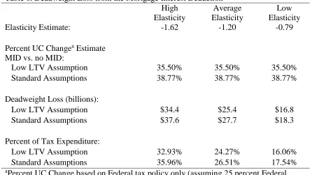
Table 6 shows deadweight loss estimates for a range of elasticity values (max, min, and
average of the empirical estimates), and for both standard (0.8) and low (0.71) loan to value
(LTV) ratios. Table 6 also shows the percentage change in user cost created by the federal MID.
Using the standard user cost assumptions and the Poterba and Sinai (2011) model, the MID is
responsible for a 39 percent reduction in annual user cost. Using the lower LTV parameter
produces a slightly smaller user cost change of 36 percent.17 The deadweight loss estimates are
also somewhat sensitive to the LTV choice, but are mainly driven by the elasticity.
26
Table 6. Deadweight Loss from the Mortgage Interest Deduction High
Elasticity
Average Elasticity
Low Elasticity
Elasticity Estimate: -1.62 -1.20 -0.79
Percent UC Changea Estimate MID vs. no MID:
Low LTV Assumption 35.50% 35.50% 35.50%
Standard Assumptions 38.77% 38.77% 38.77%
Deadweight Loss (billions):
Low LTV Assumption $34.4 $25.4 $16.8
Standard Assumptions $37.6 $27.7 $18.3
Percent of Tax Expenditure:
Low LTV Assumption 32.93% 24.27% 16.06%
Standard Assumptions 35.96% 26.51% 17.54%
aPercent UC Change based on Federal tax policy only (assuming 25 percent Federal
marginal tax rate).
Note: Share of income spent on housing assumed to be 25 percent following (Poterba 1992).
The minimum value for the elasticity of mortgage interest deducted (-0.79) shows a
deadweight loss of $17-18 billion annually, or about 16-18 percent of the total tax expenditure.18
Using the maximum value elasticity shows about double the amount of deadweight loss: $34-38
billion or 33-36 percent of the total tax expenditure. The average elasticity value produces
deadweight loss estimates of $25-27 billion, or 24-27 percent of total tax expenditure.
Tax Revenue
We also apply our estimates to generate tax revenue implications. We consider three
scenarios: (1) eliminating the MID altogether, (2) switching the MID to a uniform 15 percent
credit on mortgage interest and (3) capping the MID at 28 percent (rather than a tax filer’s actual
27
marginal tax rate). We maintain internal validity by computing the effects of each policy on the
seven AGI classes provided by the IRS data set separately before summing them in table 7.
First, we estimate the marginal tax rate for each AGI class to be the average of the single and
married-filing-jointly rates that would apply to the mean AGI for each class, weighted by the
proportion of filers with joint and non-joint returns in each class. This reflects the tax subsidy
received per dollar of interest deducted under current tax law. Then we compare each class’s
user cost (using the parameters given above) under the current tax law to the three alternatives
proposed above. This forms the change in cost of housing to which we apply one of four
elasticity estimates: zero (or no mortgage interest quantity adjustment) and the low, average and
high elasticity estimates from table 3.
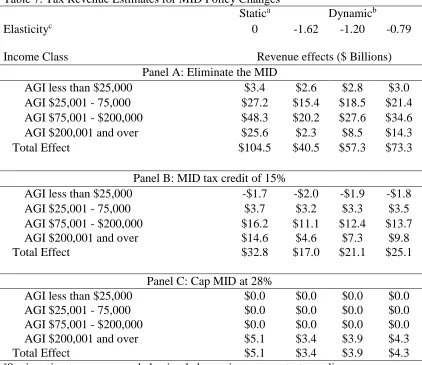
As an example, by removing the MID altogether and assuming no decrease in mortgage
interest consumption, the federal government could have raised an additional $104.5 billion in
2007. If we relax the assumption that no behavioral change will occur, the expected tax revenue
falls to a range of $41-73 billion depending on the elasticity. More specifically, we report the tax
revenue estimates as they impact each of four income groups, providing insight into the variation
driven by different income tax brackets. As expected, eliminating the MID outright causes more
revenue to be raised from earners in higher tax brackets assuming no MID quantity adjustment.
If, however, we believe earners are responsive to changes in tax policy, revenue from higher
income brackets falls off sharply at higher elasticities. The static (no adjustment) assumption
suggests earners with an AGI of less than $25,000 would pay an additional $3.4 billion versus
earners with an AGI of more than $200,001 who would pay $25.6 billion in additional taxes.
Contrast this with the high-elasticity dynamic scenario, where debt consumers are responsive to
28
Table 7. Tax Revenue Estimates for MID Policy Changes
Statica Dynamicb
Elasticityc 0 -1.62 -1.20 -0.79
Income Class Revenue effects ($ Billions)
Panel A: Eliminate the MID
AGI less than $25,000 $3.4 $2.6 $2.8 $3.0
AGI $25,001 - 75,000 $27.2 $15.4 $18.5 $21.4
AGI $75,001 - $200,000 $48.3 $20.2 $27.6 $34.6
AGI $200,001 and over $25.6 $2.3 $8.5 $14.3
Total Effect $104.5 $40.5 $57.3 $73.3
Panel B: MID tax credit of 15%
AGI less than $25,000 -$1.7 -$2.0 -$1.9 -$1.8
AGI $25,001 - 75,000 $3.7 $3.2 $3.3 $3.5
AGI $75,001 - $200,000 $16.2 $11.1 $12.4 $13.7
AGI $200,001 and over $14.6 $4.6 $7.3 $9.8
Total Effect $32.8 $17.0 $21.1 $25.1
Panel C: Cap MID at 28%
AGI less than $25,000 $0.0 $0.0 $0.0 $0.0
AGI $25,001 - 75,000 $0.0 $0.0 $0.0 $0.0
AGI $75,001 - $200,000 $0.0 $0.0 $0.0 $0.0
AGI $200,001 and over $5.1 $3.4 $3.9 $4.3
Total Effect $5.1 $3.4 $3.9 $4.3
aStatic estimates assume no behavioral change in response to tax policy.
bDynamic estimates incorporate behavior through elasticity operating on the change
in user cost.
cElasticities given are the low, average and high values derived from table 5.
29
than the highest ($2.2 billion) in additional taxes. This reflects the large incentive high earners
have to shift their debt consumption.
Our model estimates substantial revenue gains from switching the MID to a 15 percent
tax credit. Switching the MID to a tax credit has been advocated recently by the
Simpson-Bowles Debt Commission, and in the past by President Bush’s Tax Reform Panel. Revenue
gains from the switch to a credit come despite using a dynamic estimate that allows for more
mortgage interest to be deducted by lower income tax filers. The credit achieves such gains by
raising more revenue from the higher income classes (primarily those with income over
$75,001). It even reduces the tax burden on those with an AGI of less than $25,000 by nearly $2
billion. This simulation does not consider how making a new tax credit refundable would
change these revenue estimates, but we expect the revenue reductions to be modest, as
refundability would presumably also be limited to mortgages of a smaller size than the current $1
million limit.
The increase in revenues due to capping the MID at 28 percent is comparably quite low,
between $3.4 and 5.1 billion depending on the elasticity estimate used. This reflects the fact that
such a policy would only affect taxpayers in higher brackets, and only by the relatively small
difference between 28 percent and the top tax brackets. The results for all three tax law changes
are summarized in table 7.19
A key implication of these estimates is the relative uncertainty of the implications of tax
policy changes. Even with the novel data available to us, the estimates of elasticity range
widely. Table 7 should therefore be cautiously interpreted as an example of the possible changes
30
to tax revenue using elasticities that vary somewhat widely. No single number presents itself as
a take-away conclusion without making strong assumptions about which elasticity is correct.
Table 7 is more useful to illustrate the pattern of impact that might result from a change in tax
policy on different income classes, and to compare the relative impact of different tax policies.
6. Conclusion
This paper estimates the distortions caused by the mortgage interest deduction. Using
IRS data at the ZIP code level data we are able to exploit state variations in the availability of the
mortgage interest deduction using both weighted least squares regression and IV estimation. We
found relatively consistent estimates of the total change in mortgage interest deducted across
these estimates. Our results show that a one percentage point increase in the tax rate that applies
to deductibility increases the amount of mortgage interest deducted by $303–590. Employing a
user cost model we find this translates to elasticities of mortgage interest deducted with respect
to the after-tax cost of housing between -0.79 and -1.62, and deadweight loss estimates ranging
from 16-36 percent of MID tax expenditure.
Our approach to measuring deadweight loss from the MID examines the net effect of the
policy and incorporates the wide array of potential distortions that it may cause, rather than
examining the more narrow outcomes highlighted in previous work. This is a useful addition to
specific-choice estimation because it does not rely on the precision of theory behind specific
choices – regardless of the motivating factors, our estimate captures the entire effect of tax policy
on the quantity decision it is aimed at: the selection of mortgage interest to pay. All of these
choices factor into the deadweight loss of the deduction itself, and all of them are wrapped up in
31
Our elasticities imply that previous estimates of the tax revenue generated by a reduction
in the MID that do not account for full behavioral change are too large. The tax revenue
estimates given in table 7 provide a map for the relative magnitude of revenues gained when
considering behavioral change under several policies. Notably our estimates for switching to a
tax credit generate a surprising amount of revenue and expand ownership incentives to lower
income tax payers. Our work also suggests that the MID is likely to be a more substantial drag
on economic efficiency than previous estimates suggest, as we show larger elasticities that
account for behavioral change across several dimensions. The idea that the MID causes
inefficiency is inherently tied to two ideas: that imputed rents should be taxed according to a
Haig-Simons view of income, and that the MID does not encourage homeownership on the
margin (and that homeownership creates a positive externality). The most recent empirical
evidence (Hanson 2012b) suggests that the MID does not encourage homeownership. We view
taxing imputed rents as a way to make the MID an appropriate tax policy, although we question
32
Chapter II
The Impact of Housing Tax Preferences on Home Values and Neighborhood Sorting
1. Introduction
The mortgage interest deduction (MID) is a significant tax benefit to homeowners. The
Congressional Budget Office estimates that the MID cost $70 billion in foregone tax revenues in
2013, or nearly half a percent of GDP (Congressional Budget Office 2013). In 2011 it was
claimed by twenty-five percent of all tax filers. A variety of studies suggest that, to varying
degrees, the MID encourages debt financing (Dunsky and Follain 1997; Dunsky and Follain
2000; Hendershott and Pryce 2006; Poterba and Sinai 2011), buying larger homes (Hanson
2012b), and becoming owners rather than renters (Green and Vandell 1999b). Much of this
literature is focused on either the tax consequences or the behavioral impacts of the MID reform.
Previous work provides little discussion of the MID’s impact on home prices, yet
consumers, bankers and policymakers are likely to view a change in housing prices as among the
most significant consequences of reforming the MID. Home equity is a significant component of
homeowner wealth, and changes to home values would impact a household’s current and future
spending ability. The price effects of MID reform can be thought of as an adjustment cost of
correcting what is generally seen as a market-distorting tax subsidy, and they do not fall evenly
across space. This paper simulates the price effects of MID reform across a set of cities, and at
the neighborhood level within select cities, advancing the literature in several ways.
First, this study simulates average home price effects for twenty-seven different metro
areas as well as neighborhood-level effects in nineteen metro areas. Using city- and ZIP
code-level data on housing, I simulate changes to local housing prices for three different policy
33
credit, and capping the MID at a rate of fifteen percent. I find that simulated price changes vary
substantially from city to city: eliminating the MID results in an average home price decline in
Washington, D.C. of 15.7 percent, whereas the average home price in Memphis, TN would fall
by only 3.2 percent. Price changes also vary substantially between policies. For instance,
converting the MID to a fifteen percent refundable credit would reduce prices in Washington,
D.C. by only 0.6 percent and raise the average price in Memphis by 9.4 percent. In addition,
simulations at the neighborhood level reveal substantial variation in price changes within a metro
area due to sharp differences in characteristics among neighborhoods.
Second, it provides empirical support for the idea that the MID induces neighborhood
sorting on income; this result follows from the simulated neighborhood-level price effects.
While previous studies have observed that the marginal benefits of the MID increase with
income level (Glaeser and Shapiro 2003; Hanson and Martin 2014), this study examines the
distributional impact of the MID in a spatial setting.20 I break neighborhoods into income
quartiles and compute an average “affordability gap,” or the increase in user cost necessary for
the median household in a given income quartile to move to the median home one quartile higher
within the same city. I find that the average affordability gap shrinks under each reform, in one
case by as much as 17.7 percent. This implies that, by preferentially subsidizing wealthy
households, the MID also subsidizes household sorting by income across neighborhoods.
Third, it estimates key parameters in the user cost model of housing in order to calibrate
it. This model is used extensively in the public finance and real estate literatures to describe
housing costs, yet its parameters are often either taken on assumption or proxy values are used.
One troublesome parameter is the expected home price inflation rate; I use spatial variation to
34
produce a first-order coefficient for the proxy of long-run historic price inflation, which I use to
improve price predictions in the model. I also estimate the degree to which homeowners view
local property tax as an excise tax (rather than a benefit tax). The public finance literature
remains unsettled on this question; previous studies that incorporate this feature in a user cost
model typically assume a value.
Finally, it estimates behavioral adjustments to MID policy change on two dimensions: the
propensity of tax filers to itemize deductions and the degree to which homeowners utilize debt
financing in response to changes in the MID. Taking account of these behavioral adjustments in
price simulations results in differences of up to 1.9 percentage points from a set of simulations
that ignore behavioral adjustments.
The paper proceeds as follows: section 2 describes prior related work; section 3 discusses
the theoretical underpinnings of the model; section 4 briefly describes the data; section 5
describes how the model is adjusted to simulate specific policy changes; section 6 explains the
identification strategy for estimated parameters; section 7 presents the results; section 8 provides
discussion and concludes.
2. Background and Related Literature
In the growing literature on the effects of the MID, many focus on the tax expenditure of
reforming the MID or the behavioral impacts of the policy (Dunsky and Follain 1997; Green and
Vandell 1999b; Dunsky and Follain 2000; Poterba and Sinai 2011; Hanson 2012b; Hanson and
Martin 2014). Gyourko and Sinai (2003; 2004) discuss the spatial pattern of the benefits
received from tax preference. In each of these studies, price effects are secondary if they are