Climate change and sectors of the surface water cycle In CMIP5 projections

www.hydrol-earth-syst-sci.net/18/5317/2014/ doi:10.5194/hess-18-5317-2014

© Author(s) 2014. CC Attribution 3.0 License.

Climate change and sectors of the surface water

cycle In CMIP5 projections

P. A. Dirmeyer, G. Fang, Z. Wang, P. Yadav, and A. Milton

George Mason University, 4400 University Drive, MS 6C5, Fairfax VA 22030, USA

Correspondence to: P. A. Dirmeyer (pdirmeye@gmu.edu)

Received: 27 June 2014 – Published in Hydrol. Earth Syst. Sci. Discuss.: 25 July 2014 Revised: – – Accepted: 24 November 2014 – Published: 19 December 2014

Abstract. Results from 10 global climate change models are synthesized to investigate changes in extremes, defined as wettest and driest deciles in precipitation, soil moisture and runoff based on each model’s historical 20th century sim-ulated climatology. Under a moderate warming scenario, re-gional increases in drought frequency are found with little in-crease in floods. For more severe warming, both drought and flood become much more prevalent, with nearly the entire globe significantly affected. Soil moisture changes tend to-ward drying, while runoff trends toto-ward flood. To determine how different sectors of society dependent on various com-ponents of the surface water cycle may be affected, changes in monthly means and interannual variability are compared to data sets of crop distribution and river basin boundaries. For precipitation, changes in interannual variability can be important even when there is little change in the long-term mean. Over 20 % of the globe is projected to experience a combination of reduced precipitation and increased variabil-ity under severe warming. There are large differences in the vulnerability of different types of crops, depending on their spatial distributions. Increases in soil moisture variability are again found to be a threat even where soil moisture is not pro-jected to decrease. The combination of increased variability and greater annual discharge over many basins portends in-creased risk of river flooding, although a number of basins are projected to suffer surface water shortages.

1 Introduction

The suite of climate model simulations from the Coupled Model Intercomparison Project Phase 5 (CMIP5) offers a wealth of information about the potential for future climate

change across a range of emission/mitigation scenarios. The CMIP5 simulations have suggested that hydrologic feed-backs of the land surface to the atmosphere are likely to in-tensify and the spatial and temporal extent of the regions of strong feedbacks will expand in the 21st century (Dirmeyer et al., 2013, 2014). Land–atmosphere interactions are stud-ied because of their potential implications for climate dictability and their role in hydrologic extremes. These pre-vious results motivate us to examine how extremes in the sur-face water cycle are projected to change in the next century, and how they may affect specific sectors of society.

Recent studies have used the output of a small number of CMIP5 models to drive an additional suite of sector mod-els to assess changes in the likelihood of flood (Dankers et al., 2014), drought (Prudhomme et al., 2014), significant wa-ter resource impacts (Schewe et al., 2014) and agriculture (Rosenzweig et al., 2014). In such a two-step modeling ap-proach, versions of the same land surface model are some-times employed twice (once in the CMIP5 climate model and again as a sector model) or different land surface models are convolved where inconsistencies can amplify errors (cf. Koster et al., 2009).

study: meteorological (precipitation), hydrological (runoff) and agricultural (soil moisture).

Section 2 describes the data sets used and the specific anal-yses applied to those data in this study. Changes in the occur-rence rates of extremes are presented in Sect. 3. Section 4 cat-egorizes projected hydrologic changes in terms of the sectors defined above. Rainfall changes are assessed based on the spectrum of various climate indices. Soil moisture changes are composited against the global coverage of various types of crops, suggesting possible impacts on agriculture. Runoff changes are integrated over large river basins to assess im-pacts on water resources. A discussion of caveats for this study is given in Sect. 5, and a summary is presented in Sect. 6.

2 Data and analyses

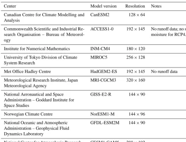
Monthly mean fields of precipitation, total runoff and mois-ture in the uppermost 10 cm of the soil from CMIP5 simula-tions (Taylor et al., 2012) are examined, along with averages of interannual standard deviation (IASD) based on monthly means. Data are taken from single simulations of 10 differ-ent climate models, the first ensemble member in each case (r1i1p1). The 10 models are listed in Table 1. Three different climate cases are considered: the transient 20th century (his-torical) case as well as two of the future climate scenarios – net radiative forcing scenarios of 4.5 Wm−2(RCP45) and 8.5 Wm−2(RCP85) (van Vuuren et al., 2011). Output from the last 90 simulated years of the three different climate cases of each model are detrended before interannual variances are calculated, as described in Dirmeyer et al. (2014). All anal-yses are performed on each model’s native grid on a month-by-month basis, and then aggregated to standard 3-month seasons by averaging the results across the 3 months, or ag-gregated across growing seasons for the crop-based analysis as explained below. Only multi-model statistics are shown – all multi-model means are a simple average of the indicated statistic across the 10 models.

Historical thresholds for extremes are defined for each model and month at each land surface grid box. Specifically, the extreme deciles are calculated from the last 90 years of un-detrended data from the historical case; the thresholds would be the values for the ninth driest and ninth wettest value for each month at each point. This defines for this study the contemporary 20th century definitions of “drought” and “flood” as represented by each model for each month of the year. These thresholds are then compared to the distri-butions derived from the RCP4.5 and RCP8.5 cases; that is, we determine how many years out of 90 exceed the histor-ical thresholds. Large changes indicate areas where adapta-tion will be critical for future water resources. Calculaadapta-tions are performed for each month and then averaged to derive estimates for 3-month seasons.

As explained in Dirmeyer et al. (2013), data from each model is interpolated onto a high-resolution global grid be-fore being combined into multi-model analyses. This avoids loss of information in the process of interpolation to a lower resolution grid than some models, or between offset grids of a similar resolution. However, the results should still be in-terpreted as representative of variability at the resolution of the climate models. We use only data over land from each model based on each model’s land–sea mask, and retain data on the high-resolution grid only where at least 8 of the 10 models have land.

For the hydrologic sector analysis, the CMIP5 data are in-terpolated onto the 1/2◦grid of the Total Runoff Integrated Pathways (TRIP) river routing data set of Oki et al. (1999). TRIP is also used to define the 100 largest named river basins for basin-scale assessments. For the agricultural sector anal-ysis, the high-resolution grid matches the 1/12◦_{gridded crop} information of Sacks et al. (2010). This is also the data set used for the global distribution of 19 major types of crops, as well as the mean planting and harvest dates. As explained in the documentation for that data set, crop calendar data were not available for all locations where each crop is grown. Ex-trapolated planting and harvest dates are provided that fill out the global grid. This information is used to define the grow-ing season at each location so that totals, averages and IASD of the multi-model water cycle variables can be calculated for the growing season. Fields for extremes in the meteoro-logical sector (precipitation) are also analyzed on the grid of Sacks et al. (2010).

3 Changes in extremes

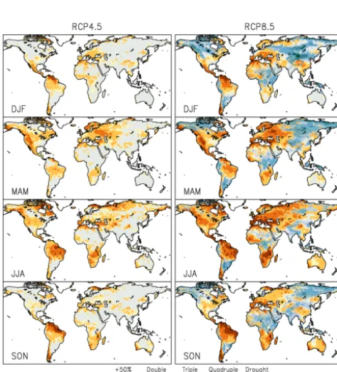
Figure 1 shows the multi-model estimates for the changes in occurrence of droughts and floods in precipitation. Shading indicates where the 20th century thresholds are exceeded at least 50, 100 (double), 200 (triple) and 300 (quadruple) per-cent more often than in the historical case (effectively 13.5, 18, 27 and 36 out of 90 years). Bootstrap tests of sampling with replacement over 104 time series simulations suggest the likelihood of falsely exceeding 50, 100 and 200 % in-creases in frequency of a 10 % tail with a sample size of 90 are 7.6, 0.7 and less than 0.01 %, respectively. There are some locations where both extremes become notably more frequent; the color scales overlap in those locations (e.g., south-central Amazon during JJA).

Table 1. CMIP5 models used in this paper.

Center Model version Resolution Notes

Canadian Centre for Climate Modelling and Analysis

CanESM2 128×64

Commonwealth Scientific and Industrial Re-search Organisation – Bureau of Meteorol-ogy

ACCESS1-0 192×145 No runoff data; no soil moisture for RCP4.5

Institute for Numerical Mathematics INM-CM4 180×120

University of Tokyo Division of Climate System Research

MIROC5 256×128

Met Office Hadley Centre HadGEM2-ES 192×145 No runoff data

Meteorological Research Institute, Japan Meteorological Agency

MRI-CGCM3 320×160

National Aeronautical and Space Administration – Goddard Institute for Space Studies

GISS-E2-R 144×90

Norwegian Climate Centre NorESM1-M 144×96

National Oceanic and Atmospheric Administration – Geophysical Fluid Dynamics Laboratory

GFDL-ESM2M 144×90

National Center for Atmospheric Research CESM1-CAM5 288×192

In the RCP8.5 case, there is hardly a region or season that is not projected to experience a marked change in precipi-tation extremes. There are widespread increases in flood fre-quency at higher latitudes of the Northern Hemisphere, peak-ing in area and severity durpeak-ing DJF. Increases are also pro-jected throughout most or all of the year over much of tropi-cal Africa and extratropitropi-cal South America, the Pacific coasts of Colombia, Ecuador and Peru, Indonesia, South Asia and Tibet. Otherwise, the regions of more pervasive drought in RCP4.5 intensify and expand.

These changes are largely reflected in soil moisture as well (Fig. 2), with a shift in the zero line relative to the precipitation changes toward more drought area, reflecting the increase in evaporation that accompanies warmer tem-peratures. A number of agriculturally important locations are seen to suffer a doubling or tripling of drought in the RCP4.5 case, and even a quadrupling or more in the RCP8.5 case. Such areas include much of eastern Europe in spring, the Great Plains of North America in summer, and the Mediter-ranean region year-round. Most agricultural areas of South and East Asia appear to escape escalation in drought in the RCP4.5 case, but China and Southeast Asia begin to succumb in RCP8.5. Tropical South America and southern Africa ap-pear to be hard-hit in both scenarios. Wet extremes in soil moisture become much more frequent across India and sur-rounding nations during and after the monsoon. It is not im-mediately clear whether this would be helpful or disruptive

for agriculture – consequences would likely depend on the location, character of the precipitation and crops grown.

Figure 3 shows the basin-average changes in the frequency of drought and flood for the 100 largest named river basins in the TRIP data set. In RCP4.5 there is only one instance of a basin having at least a 50 % increase in flood situations – the Yukon in DJF. Otherwise, the drought regions evident in precipitation are reflected here, particularly over north-ern South America, southnorth-ern North America, southnorth-ern Eu-rope and parts of Africa. Whereas changes in soil moisture extremes skew toward drought relative to the precipitation changes, runoff extremes tend more strongly toward flood. This difference is symptomatic of the projected changes in precipitation rates toward more intense rainfall events sep-arated by more severe dry periods. The change in the fre-quency distribution of precipitation favors runoff increases and reduces infiltration. Combined with greater evaporative stresses, soil moisture easily becomes depleted.

Figure 1. Multi-model estimates of change in exceedance of 10 %

(drought) and 90 % (flood) monthly precipitation totals in the RCP4.5 case (left) and RCP8.5 case (right), based on the historical simulation climatologies, for the indicated seasons. “Double” indi-cates twice as many months exceed the historical 10 % threshold for the tail of the distribution, “triple” is three times, etc.

Figure 2. As in Fig. 1 for moisture in top 10 cm of soil.

Figure 3. As in Fig. 1 for basin-average runoff from the 100 largest

river basins.

area where flood extremes increase by 5 or more years from RCP4.5 to RCP8.5 covers nearly the entire globe for each season and variable, even soil moisture (not shown). There are no locations where the multi-model estimates for flood extremes dropped by more than four cases per 90 years for any of the variables examined.

4 Sector impacts

Here we present tailored examinations of the meteorological (precipitation), agricultural (soil moisture) and hydrological (runoff) sectors.

4.1 The meteorological sector

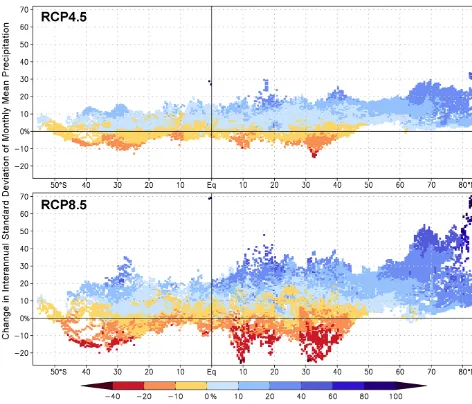
Figure 4. Scatter diagram of the change from the historical case to

the indicated future climate projection of the annual mean precipi-tation (color) and average IASD of monthly mean precipiprecipi-tation (y

axis) for all land points as a function of latitude. Each mark is a grid box on the interpolated high-resolution grid. All changes are expressed as a percentage of the climatological value from the his-torical case.

corresponding change in annual mean precipitation for each corresponding grid point.

A number of noteworthy features are evident in this fig-ure. First, as one might expect, the range of changes in both mean precipitation and its variability are generally larger in the RCP8.5 case than in RCP4.5. Second, there is a strong correspondence between the changes in mean and variance – the blue colors tend to appear for the larger changes of IASD, and the redder colors are for the small and negative changes. North of about 50◦N, nearly all locations are projected to have increases in both the mean and variability of precipita-tion.

From the standpoint of impacts, the most important fea-ture may be the preponderance of points above the x axis that are shaded orange or red. These indicate locations where mean precipitation is projected to decrease but interannual variability will increase. This is a particularly troubling com-bination, as it suggests both less reliability and less avail-ability of water from precipitation sources in these locations. The extent and magnitude of changes of this type are greater in the RCP8.5 case. By contrast, there are almost no points below the x axis that are in shades of blue – few locations are projected to have both more abundant and less variable precipitation.

Figure 5 shows the spatial distribution of locations that are projected to have, in the RCP8.5 case, a decrease of mean precipitation and an increase in interannual variability. Shad-ing denotes the average change in the IASD of monthly

pre-Figure 5. Change from the historical to the RCP8.5 case in the

aver-age IASD of monthly mean precipitation shown only for locations where it is positive but the change in annual mean precipitation is negative.

cipitation – the ordinate of Fig. 4. Locations are masked out (shaded white) where either precipitation is projected to in-crease or variability will dein-crease. The shaded regions can be interpreted as areas of particular vulnerability, quantified specifically from the meteorological sector of the water cy-cle. They cover more than 20 % of the land area, exclud-ing Antarctica. Of course, regions that are projected to ex-perience sharp declines in precipitation are vulnerable even with decreases in variability (e.g., much of the Mediterranean coast), but they are not included in this metric.

4.2 The agricultural sector

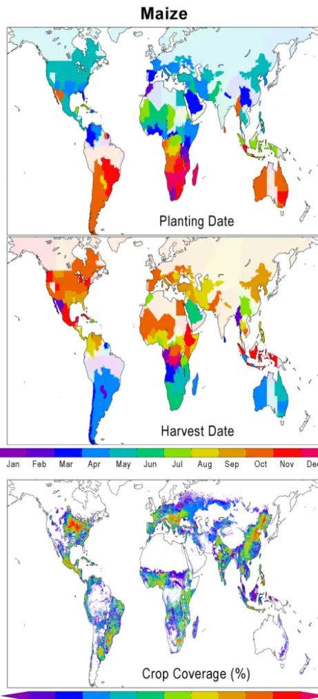
For the agricultural sector, we examine the projected changes in soil moisture in areas where crops are grown. Figure 6 shows an example of crop data from Sacks et al. (2010) for maize. Planting and harvest date data, and thus growing sea-son definitions, are primarily defined within political bound-aries in this data set for contemporary conditions (see Sect. 5 for a thorough discussion of caveats). The mean dates are used in each case; data on the range of start and end dates are also available, but we assume that they amount to random variations that will not affect the aggregate statistics. Faint shading indicates where dates in the data set were extrap-olated to fill in regions of missing data. The coverage map (upper right) is used to generate area-weighted global means of growing season mean top 10 cm soil moisture and IASD (based on monthly values) for each crop.

Table 2. Crop coverage-weighted statistics of mean and interannual standard deviation (IASD) of top 10 cm soil moisture [kg m−2] during the 20th century (hist.) and projected changes [%] from multi-model averages of 10 CMIP5 models. Changes of more than±3 % are bold.

Crop Area Mean Change Change IASD Change Change

type [103km2] (hist.) (RCP4.5) (RCP8.5) (hist.) (RCP4.5) (RCP4.5)

Wheat 2092 20.8 −2.1 % −4.5 % 3.5 +0.1 % −1.1 %

Rice 1526 27.9 +0.4% −0.2 % 3.3 +0.9% +4.5 %

Maize 1361 24.9 −2.2 % −4.6 % 3.6 +1.3% +2.6% Soybeans 746 25.8 −1.5 % −3.3 % 3.8 +2.0% +3.6 %

Pulses 671 21.6 −0.5 % −1.5 % 3.3 +0.2% +1.6%

Barley 543 21.0 −3.3 % −8.2 % 3.3 −0.1 % −1.3 %

Sorghum 389 21.2 −0.9 % −2.7 % 3.4 +1.7% +3.5 %

Millet 334 17.7 −0.6 % −1.6 % 3.2 +0.3% +1.8% Cotton 305 19.7 −0.8 % −1.2 % 3.5 +0.6% +2.3% Rapeseed 246 25.4 −1.1 % −2.2 % 3.4 −0.7 % +0.1% Groundnuts 222 22.6 −0.1 % −0.8 % 3.5 +1.0% +3.3 %

Sunflower 204 20.2 −1.9 % −6.8 % 3.5 −0.4 % −3.0 %

Potatoes 193 24.1 −2.1 % −5.2 % 3.4 +1.8% +2.4% Cassava 155 25.7 −0.8 % −2.1 % 2.8 +1.9% +6.5 %

Oats 132 22.2 −2.8 % −7.9 % 3.5 −0.1 % −1.1 %

Winter rye 94 28.5 −2.5 % −5.6 % 3.4 −1.1 % −4.4 %

Sweet potatoes 91 26.6 −0.6 % −1.4 % 3.3 +2.7% +7.1 %

Sugarbeets 61 21.7 −3.7 % −9.9 % 3.4 +0.9% −1.0 %

Yams 36 24.9 −0.6 % −2.7 % 2.3 +2.4% +9.7 %

statistical significance, so changes of more than 3 % in both metrics are highlighted in bold.

Several features stand out. There is again a strong but not universal tendency for the RCP8.5 case to show greater changes than the RCP4.5 case. Almost all area-averaged changes are negative, although maps of the changes show regions of both increasing and decreasing soil moisture in every instance. The greatest soil moisture decreases for both RCP4.5 and RCP8.5 cases are for barley and sugarbeets, both primarily European crops. Much of Europe suffers widespread precipitation decreases during summer in nearly all models (Dirmeyer et al., 2013), contributing to the drier soils. Rice, groundnuts, sweet potatoes, pulses and cotton are among the least affected crops in the global mean. While drier conditions are often not a favorable change for sustain-ing existsustain-ing agriculture, increases in year-to-year variations in moisture are particularly detrimental. Fourteen of 19 crops are projected to experience greater interannual variability of soil moisture under the RCP4.5 scenario, and 13 of 19 in the RCP8.5 case, with all increases of more than 3 % occurring in RCP8.5. The most strongly affected crops are projected to be tropical varieties: yams, sweet potatoes and cassava. Rice is also projected to experience increases in soil moisture IASD of nearly 5 % on average in the RCP8.5 case, even though mean soil moisture changes little. Winter rye and sunflower are forecast to have decreases of at least 3 % in both the mean and IASD of soil moisture.

To quantify further how soil moisture may change, cu-mulative probability distributions have been calculated. The

distributions are calculated spatially across the growing re-gions of each crop using the time mean soil moisture values, weighted by fractional coverage. For soil moisture, we focus on the median value and the value of the lowest decile (50 and 10 % of the cumulative distributions, respectively) in the historical case, and then find what fraction of the crop areas lie below those values in the future climate cases. Values ex-ceeding 50 or 10 % respectively indicate an increased area of that cropland experiencing drier conditions. One hundred bins of equal range of soil moisture are used, chosen to span the range of values in each case. Results are shown in Table 3. Situations where the drier areas have increased in extent by 20 and 40 % are highlighted.

Again, drying is generally stronger for the RCP8.5 case. However, in terms of fractional increases in area, it is the dry tail of the distribution that often suffers the greatest im-pact. Higher latitude crops such as barley, oats, winter rye and sugarbeets show the most pronounced shifts in median soil moisture. Sunflower is also strongly affected at the dry end of the soil moisture range. Rice, sorghum, millet, cotton, rapeseed and sweet potatoes are relatively stable in terms of their overall probability distributions of mean soil moisture.

Table 3. Crop coverage-weighted multi-model estimates of median (50 %) and lowest decile (10 %) values of top 10 cm soil moisture

[kg m−2] in historical case (hist.) and the projected percentage of area that will fall below those values in two future climate scenarios. Cases where the area increases by at least 20 % (i.e., by 10 % for median, 2 % for lowest decile) are shown in bold, and cases where the area increases by at least 40 % (20 % for median, 4 % for lowest decile) are bold and underlined.

Crop Median Below Below Decile Below Below

type (hist.) (RCP4.5) (RCP8.5) (hist.) (RCP4.5) (RCP4.5)

Wheat 21.0 55 % 62 % 13.5 12 % 13 %

Rice 29.6 49 % 52 % 18.9 10 % 9 %

Maize 25.1 58 % 63 % 18.5 11 % 15 %

Soybeans 25.2 59 % 62 % 21.0 11 % 15 %

Pulses 22.0 52 % 54 % 11.6 11 % 12 %

Barley 21.9 59 % 73 % 13.7 12 % 13 %

Sorghum 21.9 53 % 56 % 12.5 10 % 11 %

Millet 16.2 51 % 52 % 10.5 11 % 11 %

Cotton 18.8 51 % 51 % 10.8 11 % 11 %

Rapeseed 28.0 49 % 54 % 13.6 11 % 10 %

Groundnuts 23.6 50 % 50 % 13.8 11 % 13 %

Sunflower 19.6 57 % 68 % 14.8 12 % 22 %

Potatoes 23.9 55 % 60 % 17.1 12 % 13 %

Cassava 26.5 51 % 55 % 19.2 12 % 14 %

Oats 22.3 62 % 75 % 17.7 13 % 19 %

Winter rye 29.1 64 % 83 % 25.6 18 % 24 %

Sweet potatoes 27.6 51 % 52 % 18.5 11 % 11 %

Sugarbeets 21.6 59 % 70 % 16.2 12 % 17 %

Yams 25.4 51 % 57 % 19.8 12 % 17 %

there are notable increases in precipitation and a smaller area of cultivation experiencing less than the lower decile of rain-fall based on the historical values. For winter rye, there is a huge increase in total evapotranspiration during the growing season, which is the main driver of soil moisture depletion. For groundnuts as well as millet, soybeans and yams, there is a notable increase in runoff at the dry end of the spec-trum, consistent with change in the nature of precipitation towards fewer, more intense events. This is also evident for the shifts in the medians, where groundnuts, millet, pulses and rice show little change in mean soil moisture even though they experience increases in median and mean rainfall, with the difference going largely to increased runoff. Low-latitude crops in particular experience lower median soil moisture even though median precipitation increases, because runoff rates also increase. Yams offer an extreme example, as me-dian precipitation increases slightly, but 68 % of the crop area in the RCP8.5 case experiences runoff higher than the his-torical median, and 57 % has lower soil moisture than the historical median. This change results in a large shift in the distribution of evapotranspiration as well, where 86 % of the yam-growing area has lower ET than the historical median. Rapeseed has little change in median soil moisture but a pos-itive shift in rainfall nearly as strong as winter rye, and like winter rye the moisture sink appears to be evapotranspiration. Overall, the greatest increases in agricultural drought fre-quency appear to affect temperate (mainly European) crops and strictly tropical crops.

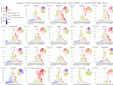
Lastly, we combine the calculation of degree of consen-sus among models for a positive verconsen-sus negative change (cf. Dirmeyer et al., 2013, 2014) with the distribution of pro-jected soil moisture changes for each crop. Figures 7 and 8 show for each crop the total area projected to have soil mois-ture changes in each of 12 ranges (6 positive, 6 negative). The coloring further shows the degree of consensus among mod-els. The pie charts summarize the percentage of each crop’s planting area in each consensus band. There is a great deal of detail in these plots, but here we only point out a few high-lights. For the RCP8.5 case (Fig. 7), four crops (barley, oats, sugarbeets and sunflower) have nearly complete consensus (>85 %) among the CMIP5 models for drier soils over more than half of their area. Most crops are dominated by drying soils. In the RCP4.5 case (Fig. 8), overall the impacts are less severe, the consensus for drying is somewhat weaker, and there is a greater but still subordinate indication for areas of wetter soils.

mod-Figure 6. Mean planting and harvest dates (indicated by month) and

the fractional coverage of each 1/12◦×1/12◦grid box of the crop maize, from the data of Sacks et al. (2010).

els (shaded green) yet a clear skew in the distribution toward decreased IASD, suggesting the multi-model results for that crop may be strongly influenced by extremes in one or two models, and uncertainty should be considered large.

4.3 The hydrological sector

Figure 10a shows the average simulated annual runoff for the 100 largest named river basins in the TRIP data set. On such long timescales, the runoff is effectively equal to pre-cipitation minus evapotranspiration. Figure 10b and c show the projected change in runoff, in percent, from historical to the RCP4.5 and RCP8.5 cases, respectively. The patterns of change are largely similar, but the magnitudes are gen-erally larger for the RCP8.5 case. There are projected de-creases in basin-scale runoff in the Americas from the south-ern United States to the subtropical region of South Amer-ica, in a band from Europe to central Asia, and across south-ern Africa. Other areas show increases, with the largest per-centage changes over northwestern Africa, high latitudes in the Northern Hemisphere, Australia and the mid-latitudes of South America.

Figure 10d, e show the changes in the IASD of runoff, calculated month by month for each model and then aver-aged across models and all months of the year, expressed in terms of standard deviations from the historical case. As with the agricultural metrics, an increase in IASD of hydrologic metrics implies less dependability and a greater propensity for extremes. Most regions show an increase in variability, including in the RCP8.5 case a number of basins in South America, Africa and Asia that show a decrease in annual runoff. The greatest percentage increases are over South Asia and western Africa.

An important tendency is revealed in Fig. 11, which shows the percentage change in the IASD scattered against the change in annual runoff for the 100 basins. The top panel is the change for the RCP4.5 case, and the bottom is for RCP8.5. The 12 largest basins are labeled and the sizes of the symbols are proportional to the ranks of the basins by area; colors simply help to differentiate the symbols. Many basins have a greater percentage increase in standard devia-tion than percentage increase in mean, indicated by the points that lie within the upper grey triangles. However, very few basins show a greater decrease in standard deviation than mean (points in the lower grey triangles). This asymmetry is reflected in the best fit linear regression through the points (solid line), which crosses the 0 % mean runoff change line at about+4.6 % change in standard deviation in the RCP4.5 case, and at +5.8 % for the RCP8.5 case. This mirrors, at the basin scale, what was found for precipitation at the point scale in Sect. 4.1; variability in the water cycle increases even when the mean is unchanged.

5 Discussion of caveats

ex-Figure 7. Probability distribution (total areas) of changes from the historical case to the RCP8.5 case in mean growing season top 10 cm soil

moisture for each crop, with the colored shading indicating the degree of consensus among models and the area of each color in the bars and pie charts proportional to the area covered by that level of consensus.

pected to affect our conclusions, but the use of monthly data increases our sample size considerably and thus confidence in the statistics. Anomalies in precipitation especially are generally uncorrelated from month to month. For the assess-ment of changes in extremes in Section 3, the choice of the 10 % tails is arbitrary and may not be an appropriate absolute threshold to define drought or flood on the monthly timescale at all locations. However, for relative comparisons there is lit-tle sensitivity to the precise choice of threshold.

The estimates of the impacts of changes to the surface water cycle on agriculture are based on static contemporary crop distributions. In reality, agriculture is constantly chang-ing and patterns of land use will adapt to changchang-ing climate as much as possible. The results on impacts to the agricultural sector should be interpreted as a measure of potential hydro-logic vulnerability to various cropping areas as they are cur-rently distributed. There are other climate change effects as well, notably temperature and atmospheric CO2, that are not considered here but have been documented elsewhere (e.g., Rosenzweig et al., 2014). The degree of crop-level impacts in this study should be interpreted as a measure of likely de-gree of need for adaptation to maintain productivity for each crop.

Furthermore, the CMIP5 models do not necessarily spec-ify the same distribution of agriculture as the crop data of Sacks et al. (2010), and none of the CMIP5 models repre-sent as many different crop types at such high spatial reso-lution. This creates numerous local inconsistencies between the observed crop distributions we have used and the type of vegetation specified in the climate models (as well as ever-present inconsistencies between models). This is also a prob-lem whenever climate model output is reapplied as forcing to component models (cf. Schellnhuber et al., 2014).

Figure 8. As in Fig. 7 but for changes from the historical case to the RCP4.5 case.

Figure 10. (a) Annual average runoff (kg m2) for the 100 largest river basins. (b) Changes (%) from historical to the RCP4.5 case and (c) the RCP8.5 case. (d) Percentage change in the IASD of monthly mean runoff averaged for all months from historical to the RCP4.5 case and (e) the RCP8.5 case.

Figure 11. Percentage change in IASD of monthly mean runoff

averaged for all months versus percentage change in annual mean runoff for the cases shown. The 12 largest river basins are labeled, and the sizes of the dots are proportional to the rank of the size of the basin. The least-squares best-fit line through the points is shown. Shading indicates the region where there is a greater percentage in-crease in standard deviation than percentage inin-crease in mean.

As with all climate studies, accuracy and the veracity of conclusions are greatest at the large scales and erode at the local scale. Given that characteristic, we emphasize as a re-sult of this study the likelihood of a great deal of variability in the impacts of climate change on different regions and facets of the meteorological, agricultural and hydrological sectors. For instance, the general conclusion is likely sound that most crops should experience drier soils and greater year-to-year variability in soil moisture, with certain crops being much more strongly affected than others. But as the spatial scale decreases, uncertainty in the projections increases.

6 Summary

mois-ture and runoff. Changes in extremes, means and interannual variability have been assessed. For the agricultural and hy-drologic sectors, climate change data have been convolved with data on crop distribution and river basin boundaries to provide targeted assessments.

Changes in extremes are defined by rates of exceedance of the driest and wettest 10 % thresholds derived from the historical 20th century simulations by each model at each grid point for each month of the year. For the RCP4.5 cli-mate projection, the only significant changes are towards in-creased drought, with northern South America appearing the most vulnerable in terms of precipitation and runoff. For soil moisture, many other areas of the globe also show marked increases in drought frequency. The drought trends intensify in the RCP8.5 case, but increased rates of flood conditions also appear around the globe. For soil moisture and runoff there are increases in both dry and wet extremes, but for soil moisture drought amplification predominates, while for runoff floods increase over more area than droughts. The pre-cipitation response lies between the other two variables, with increased drought most prevalent during JJA and flooding es-calating most during DJF.

Sector assessments show for precipitation that the pro-jected increases in interannual variability will be a major is-sue, driving the increases in extremes in all water cycle vari-ables. More than 20 % of the globe is projected to see a com-bination of increased precipitation variability and decreased mean precipitation for the RCP8.5 case – a particularly dan-gerous combination for water resources.

In the agricultural sector, soil moisture changes in the growing areas of 19 major crops show that staples pre-dominantly grown in Europe are likely to be hardest hit by drought. Many crops show offsetting regional impacts, although no attempt to account for agricultural adaptation has been made in this study. Global crops least affected by changes in mean soil moisture are rice, groundnuts, sweet potatoes, pulses and cotton. However, increased interannual variability in soil moisture is projected to affect most crops, especially in tropical areas. Figures 7 and 8 provide detailed accounting of projected impacts for each crop.

In the hydrologic sector, the increase in variability of runoff is projected to exceed changes in the mean for most river basins, despite widespread projected changes (usually increases) in annual mean discharge. This has major implica-tions for flood control, as the combination suggests increased river flooding, although droughts are projected to become more likely in many basins.

Several of the tendencies found reflect a noteworthy aspect of the water cycle in a warming climate; that is, precipitation is projected to change toward fewer but more intense events. This change reduces overall infiltration and increases surface runoff as well as its variability. It is also a contributing fac-tor in the overall reduction in soil moisture seen in Sect. 4.2. Thus, the change in precipitation statistics lies at the heart of both the drying trend in soil moisture and the trend towards

increased river basin discharge. While such results are con-sistent with theory and observations (e.g., Karl and Knight, 1998; Meehl et al., 2005; Donat et al., 2013), the degree to which the parameterizations in climate models properly rep-resent the sensitivity of precipitation processes is not well known.

Author contributions. P. A. Dirmeyer designed the analyses as part of a graduate class project for the other authors, who were students in a class on land–climate interactions at George Mason University taught by the first author. Z. Wang performed preliminary process-ing of data for all models and calculated basic statistics. G. Fang calculated the decile extremes statistics in Sect. 3. P. Yadav and A. Milton analyzed results and provided sector-based context as-sessment. P. A. Dirmeyer synthesized the sector-based results and prepared the manuscript with contributions from all co-authors.

Acknowledgements. We thank the climate modeling groups listed in Table 1 for making their model output available through the US Department of Energy’s Program for Climate Model Diagnosis and Intercomparison (PCMDI), and acknowledge the World Climate Research Programme (WCRP) Working Group on Coupled Mod-elling, which is responsible for CMIP5. The lead author’s synthesis of the student material was supported by joint funding from the Na-tional Science Foundation (ATM-0830068), the NaNa-tional Oceanic and Atmospheric Administration (NA09OAR4310058), and the National Aeronautics and Space Administration (NNX09AN50G) of the Center for Ocean Land Atmosphere Studies (COLA).

Edited by: P. Gentine

References

Dankers, R., Arnell, N. W., Clark, D. B., Falloon, P. D., Fekete, B. M., Gosling, S. N., Heinke, J., Kim, H., Masaki, Y., Satoh, Y., Stacke, T., Wada, Y., and Wisser, D.: First look at changes in flood hazard in the Inter-Sectoral Impact Model Intercompar-ison Project ensemble, Proc. Natl. Acad. Sci., 111, 3257–3261, doi:10.1073/pnas.1302078110, 2014.

Dirmeyer, P. A., Jin, Y., Singh, B., and Yan, X.: Trends in land-atmosphere interactions from CMIP5 simulations, J. Hydrome-teor., 14, 829–849, doi:10.1175/JHM-D-12-0107.1, 2013. Dirmeyer, P. A., Wang, Z., Mbuh, M. J., and Norton, H. E.:

Intensified land surface control on boundary layer growth in a changing climate, Geophys. Res. Lett., 41, 1290–1294, doi:10.1002/2013GL058826, 2014.

Karl, T. R. and Knight, R. W.: Secular trends of precipitation amount, frequency, and intensity in the United States, B. Am. Meteor. Soc., 79, 231–241, 1998.

Koster, R. D., Guo, Z., Dirmeyer, P. A., Yang, R., Mitchell, K., and Puma, M. J.: On the nature of soil moisture in land surface mod-els, J. Climate, 22, 4322–4335, doi:10.1175/2009JCLI2832.1, 2009.

Meehl, G. A., Arblaster, J. M., and Tebaldi, C.: Understand-ing future patterns of increased precipitation intensity in cli-mate model simulations, Geophys. Res. Lett., 32, L18719, doi:10.1029/2005GL023680, 2005.

Oki, T., Nishimura, T., and Dirmeyer, P.: Assessment of annual runoff from land surface models using Total Runoff Integrating Pathways (TRIP), J. Meteor. Soc. Japan, 77, 235–255, 1999. Prudhomme, C., Giuntoli, I., Robinson, E. L., Clark, D. B., Arnell,

N. W., Dankers, R., Fekete, B. M., Franssen, W., Gerten, D., Gosling, S. N., Hagemann, S., Hannah, D. M., Kim, H., Masakik, Y., Satoh, Y., Stackei, T., Wada, Y., and Wisser, D.: Hydrological droughts in the 21st century, hotspots and uncertainties from a global multimodel ensemble experiment, Proc. Natl. Acad. Sci., 111, 3262–3267, doi:10.1073/pnas.1222473110, 2014.

Rosenzweig, C., Elliott, J., Deryng, D., Ruane, A. C., Müller, C., Arneth, A., Boote, K. J., Folberth, C., Glotter, M., Khabarov, N., Neumann, K., Piontek, F., Pugh, T. A. M., Schmid, E., Ste-hfest, E., Yang„ H., and Jones, J. W.: Assessing agricultural risks of climate change in the 21st century in a global gridded crop model intercomparison, Proc. Natl. Acad. Sci., 111, 3268–3273, doi:10.1073/pnas.1222463110, 2014.

Sacks, W. J., Deryng, D., Foley, J. A., and Ramankutty, N.: Crop planting dates: an analysis of global patterns, Global Ecol. Biogeogr., 19, 607–620, doi:10.1111/j.1466-8238.2010.00551.x, 2010.

Schellnhuber, H. J., Frieler, K., and Kabat, P.: The ele-phant, the blind, and the intersectoral intercomparison of climate impacts, Proc. Natl. Acad. Sci., 111, 3225–3227, doi:10.1073/pnas.1321791111, 2014.

Schewe, J., Heinke, J., Gerten, D., Haddeland, I., Arnell, N. W., Clark, D. B., Dankers, R., Eisner, S., Fekete, B. M., Colón-González, F. J., Gosling, S. N., Kim, H., Liu, X., Masaki, Y., Portmann, F. T., Satoh, Y., Stacke, T., Tang, Q., Wada, Y., Wisser, D., Albrecht, T., Frieler, K., Piontek, F., Warszawski, L., and Kabat, P. : Multimodel assessment of water scarcity under climate change, Proc. Natl. Acad. Sci., 111, 3245–3250, doi:10.1073/pnas.1222460110, 2014.

Taylor, K. E., Stouffer, R. J., and Meehl, G. A.: An overview of CMIP5 and the experiment design, B. Am. Meteor. Soc., 93, 485–498, 2012.