Hydrol. Earth Syst. Sci., 13, 759–777, 2009 www.hydrol-earth-syst-sci.net/13/759/2009/ © Author(s) 2009. This work is distributed under the Creative Commons Attribution 3.0 License.
Hydrology and
Earth System
Sciences
Influence of thermodynamic soil and vegetation parameterizations
on the simulation of soil temperature states and surface fluxes by the
Noah LSM over a Tibetan plateau site
R. van der Velde1, Z. Su1, M. Ek2, M. Rodell3, and Y. Ma4
1International Institute for Geo-Information Science and Earth Observation (ITC), Hengelosestraat 99, P.O. Box 6, 7500 AA Enschede, The Netherlands
2Environmental Modeling Center, National Center for Environmental Prediction, Suitland, Maryland, USA 3Hydrological Science Branch, Code 614.3, NASA, Goddard Space Flight Center, Greenbelt, Maryland, USA 4Institute of Tibetan Plateau Research (ITP/CAS), P.O. Box 2871, Beijing 100085, China
Received: 21 November 2008 – Published in Hydrol. Earth Syst. Sci. Discuss.: 21 January 2009 Revised: 8 May 2009 – Accepted: 22 May 2009 – Published: 12 June 2009
Abstract. In this paper, we investigate the ability of the Noah Land Surface Model (LSM) to simulate temperature states in the soil profile and surface fluxes measured during a 7-day dry period at a micrometeorological station on the Tibetan Plateau. Adjustments in soil and vegetation parameteriza-tions required to ameliorate the Noah simulation on these two aspects are presented, which include: (1) differentiating the soil thermal properties of top- and subsoils, (2) investigation of the different numerical soil discretizations and (3) calibra-tion of the parameters utilized to describe the transpiracalibra-tion dynamics of the Plateau vegetation. Through the adjustments in the parameterization of the soil thermal properties (STP) simulation of the soil heat transfer is improved, which results in a reduction of Root Mean Squared Differences (RMSD’s) by 14%, 18% and 49% between measured and simulated skin, 5-cm and 25-cm soil temperatures, respectively. Fur-ther, decreasing the minimum stomatal resistance (Rc,min) and the optimum temperature for transpiration (Topt) of the vegetation parameterization reduces RMSD’s between mea-sured and simulated energy balance components by 30%, 20% and 5% for the sensible, latent and soil heat flux, re-spectively.
Correspondence to: R. van der Velde
1 Introduction
An accurate characterization of the heat and moisture ex-change between the land surface and atmosphere is impor-tant for Atmospheric General Circulation Models (AGCM) to forecast weather at various time scales (i.e. McCumber and Pielke, 1981; Garratt, 1993; Koster et al., 2004). Within op-erational AGCM these land-atmosphere interactions are de-scribed by a Land Surface Model (LSM). Because AGCM are computationally demanding, numerical efficiency of the LSM is required. Therefore, a simplified implementation of the physical processes and the applied parameterizations are inevitable. For example, the impact of a physically based for-mulation of roughness lengths for momentum and heat trans-port on the calculation of the surface fluxes has been stressed (i.e. Chen et al., 1997; Zeng and Dickinson, 1998; Su et al., 2001; Liu et al., 2007; Ma et al., 2008) and the influence of a more detailed description of the land surface hydrology has been discussed (i.e. Gutmann and Small, 2007; Gulden et al., 2007). Furthermore, a limited number of soil and vege-tation parameterizations are accommodated in modeling sys-tems operational at a global scale (e.g. Ek et al., 2003).
which showed that thorough optimization of a comprehen-sive set of model parameters, can reduce differences be-tween the measured and simulated heat fluxes for the semi-arid Walnut Gulch watershed (Arizona, USA) by as much as 20–40 W m−2. The investigation by Dickinson et al. (2006) demonstrates the existence of inconsistencies in the simula-tions of land surface processes, while Hogue et al. (2005) show that through adjustment of the LSM parameterizations an improvement is obtained in the model’s performance. This suggests that even for extreme environment the imple-mented LSM physics is flexible enough to represent the land surface processes adequately given the appropriate parame-terization.
Within the framework of the Model Parameter Estimation Experiment (MOPEX) the development of area specific land surface parameterization has been accommodated (Schaake et al., 2006). The focus of this initiative has been on the de-velopment parameter estimation methodologies and the cali-bration of parameters that affect primarily the rainfall-runoff relationships (Duan et al., 2006). As a result, the influence of model parameters on simulation of surface energy bal-ance has received little attention within MOPEX. One of the few investigations that addressed the impact parameter un-certainty on energy balance simulations has been reported by Kahan et al. (2006). They showed for the Simplified Simple Biosphere (SSiB, Xue et al., 1991) model that adjustment in the Leaf Area Index (LAI), stomatal resistance and satu-rated hydraulic conductivity (Ksat) are required to decrease systematic differences between simulated and measured sen-sible and latent heat fluxes for a Sahelian study area in Niger. Moreover, the importance of proper thermal diffusivity is emphasized in order to reduce uncertainties in the simulated diurnal evolution of the surface temperature and sensible heat flux. In a MOPEX-related study, Yang et al. (2005) have shown for the Tibetan Plateau that also the vertical soil het-erogeneity may have a significant impact on the partitioning of radiation.
These previous investigations demonstrate that adjust-ments in soil and vegetation parameterizations can yield sig-nificant improvements in the simulation of the surface en-ergy balance. They also emphasize the need to analyze pa-rameter uncertainties of different LSM’s in more detail. In this context, the Noah LSM is employed to simulate the land surface process of a Tibetan Plateau site for a 7-day dry pe-riod (3 September to 10 September 2005) during the Asian Monsoon. The objective of this study is to identify the ad-justments in soil and vegetation parameterizations needed to reconstruct the temperature states in the soil profile and the measured surface energy fluxes over this short period. In this paper, firstly, the results of Noah simulations obtained by us-ing standard parameterizations employed for application at global scales are presented. Secondly, the adjustments in the soil and vegetation parameterizations are explored to opti-mize the model performance.
2 Data set
2.1 Study site
The study site selected for this investigation is the micro-meteorological Naqu station located (31.3686◦N, 91.8987◦E) approximately 25 km southwest of Naqu city. This station is part of the meso-scale observational network previously installed in the Naqu river basin in the framework of the GAME (GEWEX (Global Energy and Water cycle Ex-periment) Asian Monsoon ExEx-periment) and CAMP (CEOP (Coordinated Enhanced Observing Period) Asia-Australia Monsoon Project) Tibet field campaigns. The heat flux mea-surements collected during these field campaigns have been extensively used to improve the understanding on the wa-ter and energy exchange between the land surface and atmo-sphere over the Tibetan Plateau (e.g. Ma et al., 2002, 2005; Yang et al., 2005, 2008).
In Fig. 1 a subset of a LandSat TM false color image is shown covering a part of the watershed and indicating the location of the study site. Despite the high overall al-titude (4500 m) and significant relief in some parts of this region, the terrain in the proximity of the study site is rela-tively smooth, varying only tens of meters in elevation. The weather on this part of the plateau is influenced by the warm wet monsoon in the summer and cold dry winters with tem-peratures below freezing point. Land cover consists of short prairie grasses in higher parts of the watershed and short wet-land vegetation in the local depressions. The direct environ-ment of Naqu station consists of short grasses, but within a hundred meters a wetland is situated. Based on textu-ral and hydraulic characterizations performed in the labo-ratory, the soils can be classified as sandy loam (70% sand and 10% silt) with a high saturated hydraulic conductivity (Ksat=1.2 m d−1) on top of an impermeable rock formation. Due to the high root density from the short grasses, organic matter content in the top-soils is relatively high (14.2%).
R. van der Velde et al.: Simulation of surface processes over a Tibetan plateau site 761
30
Figures:
Fig. 1: LandSat TM false color image acquired over the Tibetan study site and its approximate
location within the Tibetan Plateau.
Fig. 1. LandSat TM false color image acquired over the Tibetan study site and its approximate location within the Tibetan Plateau.
completely dry, the soil moisture measurements indicate that prior to 3 September several intensive rain events wetted the land surface. The selected period represents, thus, a typical dry-down cycle, which is, in general, a solid basis for valida-tion of LSM parameterizavalida-tions.
2.2 Surface fluxes
The soil heat flux is reconstructed using Fourier’s Law from temperature gradient measurements between the sur-face (Tskin) and the soil depth at which the first temperature measurements are made, which is 0.05 m (T5cm). This tem-perature gradient andG0are related to each other as follows,
G0=κh(sm)
∂T
∂z =κh(sm)
Tskin−Ts1
dz (1)
whereκhis the thermal conductivity [W m−1K−1], sm is soil
moisture content [m3m−3],zis the soil depth. Application of this approach requires formulation of the thermal conduc-tivity, which depends on the soil constituents, such as quartz and organic matter contents. Various scientists (e.g. de Vries, 1963; Johansen, 1975; Peters-Lidard et al., 1998) have de-veloped generic formulations to relate the soil texture to the thermal conductivity. In Hillel (1998), however, it is pointed out thatκh not merely depends on the soil constituents, but
is also affected by the size, shape and spatial arrangement of soil particles. Given the rather specific conditions on the Tibetan Plateau,κhunder the initial soil moisture conditions
(κhi) of the analyzed period is derived from the measured soil heat flux at a soil depth of 10 cm (G10)and the soil tempera-ture gradient. Using theκhi, theκhis extrapolated for
follow-ing time steps usfollow-ing the measured soil moisture accordfollow-ing to,
κh(sm)=κhi +(smi−sm) κw (2)
where, κw is the thermal conductivity of water
[=0.57 W m−1K−1], and sub- and superscript i refer to the initial conditions of the selected period.
Unfortunately, the turbulent heat fluxes measured by the eddy correlation (EC) instrumentation at Naqu station are not available for the selected period. Therefore, the sensible (H) and latent heat (λE) fluxes have been computed using the Bowen Ratio Energy Balance (BREB)– method (i.e. Perez et al., 1999; Pauwels and Samson, 2006), whereby the Bowen Ratio (β) is defined as,
β = H
λE =γ
Tair1−Tair2
eair1−eair2
(3) where,eis vapor pressure [kPa], subscripts air1 and air2 in-dicate the first and second atmospheric level, respectively, andγ is psychrometric constant [kPa K−1] defined as,
γ = cpP
0.622·λ (4)
where, cp is specific heat capacity of moist air
[=1005 kJ kg−1K1], P is the air pressure [kPa] and λ
Table 1. List of measurements conducted at Naqu station at 10-min intervals that have been used in this investigation.
Variables Instrumentation height [m] Measurement uncertainty
Air pressure PTB220C, Vaisala +1.5 m ±1 hPa
Incoming and outgoing, CM21, Kipp & Zonen +2.0 m ±0.5% at 20◦C
longwave and shortwave radiation
Wind speed WS-D32, Komatsu +1.0 m, +5.0 m, + 8.2 m ±0.8 m/su<10 m/s
±5%u >10 m/s
Humidity HMP-45D, Vaisala +1.0 m, +8.2 m ±3%
Air temperature TS-801(Pt100), Okazaki +1.0 m, +8.2 m ±3%
Soil heat flux MF-81,EKO −0.10 m ±5%
Soil temperature Pt100, Vaisala Surface,−0.05 m,−0.10 m, ±0.5◦C
−0.20 m,−0.40 m
Soil moisture 10 cm ECH2O probe, decagon devices −0.05 m,−0.20 m 0.024 cm3cm−3
Once theβhas been determined from the air temperature and vapor pressure profiles measurements theλEandHcan be calculated using,
λE=Rn−G0
1+β (5)
and
H= β
1+β (Rn−G0) (6)
The β has been computed using the air temperature and vapor pressure measurements at levels of 1.0 m and 8.2 m. As BREB-method has a limited validity whenβ approaches
−1.0, latent and sensible heat fluxes derived fromβ values between −1.3 and −0.7 have been omitted from the data analysis (e.g. Perez et al., 1999; Pauwels et al., 2008).
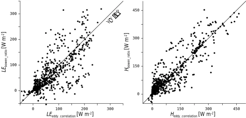
Since the reliability of BREB-method depends on the ac-curacy of the measured air temperature and humidity profile, the validity of its application to the Tibetan measurements is evaluated through comparison of the BREB-method and the measured EC heat fluxes, which are both available for the pe-riod between 16 April and 26 April 2005. Figure 2 presents the BREB-method fluxes plotted against the EC measure-ments. The figure shows, despite a large scatter, that the gen-eral pattern of data points follows the 1:1 line resulting in a Root Mean Squared Difference (RMSD) of 31.14 W m−2. A similar agreement between the BREB-method and EC heat fluxes has previously been reported by Pauwels and Sam-son (2006). We, therefore, conclude that the BREB-method derived heat fluxes are representative for the EC measure-ment and can be used to evaluate Noah’s performance.
3 Noah LSM
The Noah LSM originates from the Oregon State Univer-sity (OSU) LSM, which includes a diurnally dependent Pen-man approach for the calculation of the latent heat flux un-der non-restrictive soil moisture conditions (Marht and Ek, 1984), a simple canopy model (Pan and Marht, 1987), a four-layer soil model (Marht and Pan, 1984; Schaake et al., 1996) and a Reynolds number based approach for the determina-tion of the ratio between the roughness lengths for momen-tum and heat transport (Zilintinkevich, 1995; Chen et al., 1997). Since the National Centers for Environmental Pre-diction (NCEP) started to use the OSU LSM in their AGCM systems, the original OSU model was gradually expanded to be representative for a broader range of surface conditions and was renamed Noah. An overview of the latest changes to Noah is documented in Ek et al. (2003), which affect the cold-season processes most notably (e.g. frozen soil mois-ture, snow pack process). Also, the recent versions of Noah continue to perform well in various LSM intercomparison studies (e.g., IGPO 2002; Mitchell et al., 2004; Rodell et al., 2004; Kato et al., 2007).
3.1 Soil water movement
The soil water flow is simulated through application of the diffusivity form of Richards’ equation, which can be formu-lated as follows,
∂sm
∂t =
∂ ∂z
D (sm)∂sm
∂z
+∂K (sm)
R. van der Velde et al.: Simulation of surface processes over a Tibetan plateau site 763
31 Fig. 2: Comparison of the heat fluxes derived using the Bowen Ratio Energy Balance (BREB) method and from eddy correlation (EC) measurements for the period April 16th and
April 26th 2005; the latent heat flux is shown in the left panel and the sensible heat flux in the
right panel. The Root Mean Squared difference between the BREB and EC heat fluxes is found to be 31.14 W m-2.
0 150 300 450
Heddy_correlation [W m-2]
0 150 300 450
Hbo
w
en_
ra
ti
o
[W
m
-2]
0 100 200 300
LEeddy_correlation [W m-2]
0 100 200 300
LEbo
we
n_ra
ti
o
[W m
-2]
[image:5.595.98.493.63.253.2]1:1 li ne
Fig. 2. Comparison of the heat fluxes derived using the Bowen Ratio Energy Balance (BREB) method and from eddy correlation (EC)
measurements for the period 16 April and 26 April 2005; the latent heat flux is shown in the left panel and the sensible heat flux in the right
panel. The Root Mean Squared difference between the BREB and EC heat fluxes is found to be 31.14 W m−2.
where K is the hydraulic conductivity [m s−1], D is the soil water diffusivity [m2s−1],S is representative for sinks and sources (i.e. rainfall, dew, evaporation and transpiration) [m3m−3s−1], andt represents the time [s]. The non-linear
K-sm and D-sm relationships are defined by the formulation of Cosby et al. (1984) for 9 different soil types.
3.2 Soil heat flow
The transfer of heat through the soil column is governed by the thermal diffusion equation,
C (sm)∂T
∂t =
∂ ∂z
κh(sm)
∂T ∂z
(8) whereCis the soil moisture dependent thermal heat capac-ity [J m−3K−1], which is computed using (McCumber and Pielke, 1981),
C=fsoilCsoil+fwCw+fairCair (9)
wheref is the volume fraction of the soil matrix, and sub-scripts “soil”, “w”, “air” refer to the solid soil, water and air components. In Noah,Csoil,CairandCw are defined as
2.0·106, 1005 and 4.2·106J m−3K−1, respectively. In re-ality, Csoil depends also on the soil textural properties, but differences in the heat capacity of the soil constituents can typically be assumed to be negligible (Hillel, 1998) and are, therefore, not accounted for by Noah. For the Tibetan Plateau region, however, Yang et al. (2005) concluded that the pres-ence of roots in the top soil may alter the soil thermal prop-erties (STP) significantly.
The layer integrated form of Eq. (8) is solved using a Crank-Nicholson scheme and the temperature at the bottom
boundary is defined as the annual mean surface air tempera-ture, which is specified at a depth of 8 m. Here, for our Ti-betan study site a value of 277.25 K is used. The top bound-ary condition is confined by surface temperature, which is computed using the surface energy balance. For the calcula-tion of the surface temperature the following linearizacalcula-tion is employed,
Tskin4 ≈Tair4
1+4
T
skin−Tair
Tair
(10) Substitution of Eq. (10) into the energy balance equation yields the following expression for the surface temperature,
Tskin=Tair+
F−H−λE−G0
4Tair3
−1
4εsσ Tair (11)
with,
F =(1−α) S↓+L↓
whereαis the albedo [-],εs is the surface emissivity [-], S↓
and L↓ are the shortwave and longwave incoming radiation [W m−2], respectively. Based on measurements of the S↓ and shortwave outgoing radiation (S↑), theαis estimated to be 0.17 for the selected time period.
3.3 Surface energy balance
The surface energy budget characterized within Noah can be formulated as follows,
F −εsσ Tskin4 =H+λE+G0 (12)
whereby the κh is calculated (e.g. Johansen, 1975;
Peter-Lidard et al., 1998) as a weighted combination of the satu-rated (κsat) and dry thermal conductivity (κdry)depending on the degree of saturation according to,
κh=Ke κsat−κdry+κdry (13)
whereKeis the Kersten (1949) number representing the
de-gree of saturation determined by,
Ke =log 10
sm
smsat
+1.0 (14)
withsmsatas the saturated soil moisture content [m3m−3].
κdryis calculated using a semi-empirical equation,
κdry=
0.135γd+64.7
2700−0.947γd
(15) whereγd is the density of dry soil approximated byγd = (1−smsat)2700 [kg m−3] and κsat depends on the volume fractions of the solid particles, frozen and unfrozen soil water in the matrix,
κsat=κsoil(1−smsat)κice(1−smice)κ(
smliq)
h2o (16)
where κice and κh2o are the thermal conductivities for ice and liquid water [=2.2 and 0.57 W m−1K−1, respectively],
smice and smliq are the frozen and liquid soil water contents [m3m−3] andκsoilis the thermal conductivity of the dry soil matrix calculated as a function of the volumetric quartz frac-tion (qtz),
κsoil=κqtz(qtz)κ
(1−qtz)
o (17)
where κqtz and κo are the thermal conductivity of quartz
and others soil particles, which are set to 7.7 and 2.0 [W m−1K−1], respectively.
The sensible heat flux is calculated through application of the bulk transfer relationships (e.g. Garratt, 1993), which can be written as,
H=ρcpChu[Tskin−θair] (18)
whereρ is the air density [kg m−3], Ch is the surface
ex-change coefficient for heat [-],uis the wind speed [m s−1] andθairis the potential air temperature [K]. The surface ex-change coefficient for heat is obtained through application of the Monin-Obukhov similarity theory, whereby the ratio of the roughness length for momentum and heat transport (kB−1=ln[z0m/z0h]) is determined by the Reynolds number
dependent formulation of Zilintinkevich (1995).
Simulation of theλEis performed using a Penman-based diurnally dependent potential evaporation approach (Marht and Ek, 1984), and applying a Jarvis (1976)-type surface re-sistance parameterization similar to the one of Jacquemin and Noilhan (1990) to impose soil and atmosphere constraints to obtain the actualλE. Assuming the surface exchange co-efficient for heat (Ch) and moisture (Cq) are equivalent, the
diurnally dependent potential evaporation can be formulated as follows,
λEp=
1 (Rn−G0)+ρλCqu (qsat −q)
1+1 (19)
where1is the slope of the saturated vapour pressure curve [kPa K−1], qsat and q are the saturated and actual specific humidity [kg kg−1].
The actual λE is calculated as the sum of three compo-nents: (1) soil evaporation (Edir), (2) evaporation of inter-cepted precipitation by the canopy (Ec)and (3)
transpira-tion through the stomata of the vegetatranspira-tion (Et). The linear
method by Mahfouf and Noilhan (1991) is used to compute the soil evaporation extracted from the top soil layer, accord-ing to,
Edir=(1−fc)
sm
1−smdry
smsat−smdry
f x
Ep (20)
wherefc is the fractional vegetation cover, fx is an
empiri-cal constant taken equal to 2.0 and subscripts “1”, “sat” and “dry” indicate the soil moisture content in the first soil layer, saturated soil moisture content and wilting point [m3m−3], respectively. For our Tibetan Plateau site, thefcis assumed
to be 0.3.
The canopy evaporation is calculated using,
Ec=fcEp
cmc cmcmax
0.5
(21) where cmc and cmcmaxare the actual and maximum canopy moisture contents [kg m−2]. The canopy transpiration is de-termined by,
Et =fcPcEp
1− cmc
cmcmax 0.5
(22) wherePcis the plant coefficients defined as,
Pc =
1+ 1
Rr 1+RcCh+R1
r
(23)
withRris a function of the wind speed, air temperature,
sur-face pressure andCh, and
Rc =
Rc,min
LAIRc,radRc,tempRc,humRc,soil
(24)
where LAI is the leaf area index [m2m2],Rc,minis the min-imum stomatal resistance, andRc,rad,Rc,temp,Rc,hum,Rc,soil represent sub-optimal conditions for transpiration in term of incoming solar radiation, temperature, humidity and soil moisture, respectively, which are defined as,
Rc,rad=
Rc,min/Rc,max+ff
1+ff where ff=1.10 S↓
LAI·Rgl Rc,temp=1−0.0016 Topt−Tair
R. van der Velde et al.: Simulation of surface processes over a Tibetan plateau site 765
Table 2. Soil parameter sets defined for the 9 soil texture classes
used within large-scale Noah applications (after Cosby et al., 1984).
Soil texture class smsat ψsat Ksat b-parameter Quartz
[m3m−3] [m−1] [m d−1] [-] [-]
Loamy sand 0.421 0.04 1.22 4.26 0.82
Silty clay loam 0.464 0.62 0.17 8.72 0.10
Light clay 0.468 0.47 0.09 11.55 0.25
Sandy loam 0.434 0.14 0.45 4.74 0.60
Sandy clay 0.406 0.10 0.62 10.73 0.52
Clay loam 0.465 0.26 0.22 8.17 0.35
Sandy clay loam 0.404 0.14 0.39 6.77 0.60
Organic 0.439 0.36 0.29 5.25 0.40
Glacial/land ice 0.421 0.04 1.22 4.26 0.82
smsat ∼saturated hydraulic conductivity;
ψsat ∼soil water potential at the air entry level;
Ksat ∼saturated hydraulic conductivity;
b-parameter∼empirical parameter defining the shape of the
reten-tion curve;
Quartz∼quartz content;
Rc,hum=
1 1+hs(qsat−q)
Rc,soil = nroot
X
i=1
sm(i)−smwlt
smref−smwltfroot(i) (25)
In this formulation, smref is the soil moisture content [m3m−3] below which the simulated root water uptake and transpiration are reduced and is taken equivalent to the field capacity, nroot is the number of root zone layers,froot(i)is the fraction of the total root zone the it hlayer represents,
Rc,max is the maximum stomatal resistance, andRgl, Topt andHs are semi-empirical parameter describing the optimal
transpiration conditions with respect to the incoming solar radiation, air temperature and humidity.
3.4 Application of the Noah LSM
Description of the Noah LSM physics in the text above in-dicates that simulation requires the definition of a number of parameters. This comprehensive set of parameters can be subdivided into parameters describing the initial conditions, numerical discretization of the soil column, vegetation prop-erties, soil hydraulic and thermodynamic properties. Appli-cation of Noah in a default mode accommodates four soil layers with thicknesses of 0.1, 0.3, 0.6 and 1.0 m, respec-tively. For each layer, initial soil moisture and temperature states should be defined.
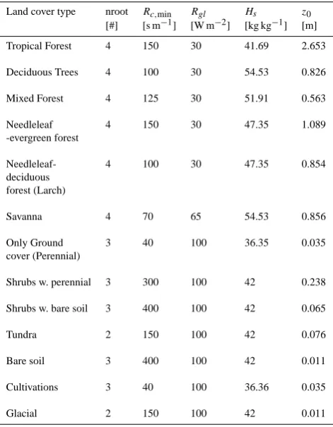
[image:7.595.48.287.99.209.2]At a global scale, 9 different texture dependent soil param-eter sets (hydraulic and thermodynamic) and 13 vegetation parameter sets are defined. The soil and vegetation parame-ter sets used within Noah are given in Tables 2 and 3. Next to the soil texture and land cover dependent parameters, sev-eral soil and vegetation parameters are assumed to be gensev-eral
Table 3. Vegetation parameter sets defined for the 13 land cover
types used within large-scale Noah applications.
Land cover type nroot Rc,min Rgl Hs z0
[#] [s m−1] [W m−2] [kg kg−1] [m]
Tropical Forest 4 150 30 41.69 2.653
Deciduous Trees 4 100 30 54.53 0.826
Mixed Forest 4 125 30 51.91 0.563
Needleleaf 4 150 30 47.35 1.089
-evergreen forest
Needleleaf- 4 100 30 47.35 0.854
deciduous forest (Larch)
Savanna 4 70 65 54.53 0.856
Only Ground 3 40 100 36.35 0.035
cover (Perennial)
Shrubs w. perennial 3 300 100 42 0.238
Shrubs w. bare soil 3 400 100 42 0.065
Tundra 2 150 100 42 0.076
Bare soil 3 400 100 42 0.011
Cultivations 3 40 100 36.36 0.035
Glacial 2 150 100 42 0.011
applicable, which are given in Table 4. Somewhat peculiar is that the Leaf Area Index (LAI) is held constant at a value of 5.0 m2m−2(see also Hogue et al., 2005) instead of using other data sources, such as the ones available from satellite platforms. In this investigation, we evaluate the Noah as it is applied at a global scale and, therefore, the default LAI value is used. The impact of this large LAI values on the results is addressed in the discussion via Noah simulations performed with a more realistic LAI, which is found to be 1.2 m2m−2 for the study site based on the Moderate Resolution Imaging Spectroradiometer (MODIS) LAI product. Further, it should be noted that by default one set of hydraulic and thermody-namic parameters is adopted for the entire soil column, and no distinction is made between the top- and subsoil.
4 Evaluation of the Noah simulations obtained using de-fault parameterizations
32 Fig. 3: Comparison of the heat fluxes measured and simulated by Noah using three default vegetation parameterizations. In the plots on the left side the measurements and simulations are presented as a time series, the right side plots show cumulative distributions.
-100 0 100 200 300 400
Sensible heat flux [W m-2]
0 0.2 0.4 0.6 0.8 1
C
um
m
ul
at
ive dist
ribution
[-]
246 248 250 252 254 256
Day of the Year [#] -200
-100 0 100 200 300 400
Soil heat fl
ux
[W
m
-2]
246 248 250 252 254 256
Day of the Year [#] -100
0 100 200 300 400
Sen
sible heat flux [W m
-2]
246 248 250 252 254 256
Day of the Year [#] -100
0 100 200 300 400
La
ten
t he
at
flux
[W
m
-2]
-200 -100 0 100 200 300 400
Soil heat flux [W m-2] 0
0.2 0.4 0.6 0.8 1
Cu
m
m
ul
ativ
e d
istribu
tio
n
[-]
-100 0 100 200 300 400
Latent heat flux [W m-2]
0 0.2 0.4 0.6 0.8 1
Cum
m
ul
ati
ve
dis
tri
bu
ti
on
[-]
[image:8.595.101.495.64.528.2]Observed Bare soil Glacial Tundra
Fig. 3. Comparison of the heat fluxes measured and simulated by Noah using three default vegetation parameterizations. In the plots on the
left side the measurements and simulations are presented as a time series, the right side plots show cumulative distributions.
conditions have been derived from in-situ measurements. The “Loamy sand” soil parameterization is adopted as be-ing equivalent to the local conditions. Due to the extreme conditions on the Tibetan Plateau, assignment of a single vegetation parameterization from the 13 default land cover types is not possible. Therefore, the Noah model is run us-ing three different vegetation parameter sets that are consid-ered equally representative for the Tibetan Plateau, which are: tundra, bare soil and glacial.
In Fig. 3 measured and simulated heat fluxes (H,λEand
R. van der Velde et al.: Simulation of surface processes over a Tibetan plateau site 767
Table 4. Soil, vegetation and other parameters assumed to be
con-stant within large-scale Noah application regardless of the soil tex-ture, land cover class and geographic location.
Parameter Description Default Value
Rc,max Maximum stomatal resistance 5000 [s m−1]
Topt Optimal temperature for transpiration 24.85 [◦C]
LAI Leaf Area Index 5.0 [m2m−2]
Csoil Soil heat capacity 2.0·106[J m−3K−1]
Czil Zilintinkevich constant 0.2 [dimensionless]
soil temperature states. The RMSD and bias are calculated using,
RMSD=
r
1
n
X
(Ot−St)2 (26)
bias=1
n
X
Ot−
1
n
X
St (27)
whereOtis the measured values at timet,Stis the simulated
value at timet andnis the total number of observations. In general, the comparison indicates that the partitioning between theH andλEis not properly simulated by Noah. Noah overestimates the measuredH resulting in biases of 41.25–52.69 W m−2 and underestimates the λE by 18.36– 39.53 W m−2depending on the adopted vegetation parame-terization. As a result of the biases obtained forH andλE, also the obtained RMSD’s are somewhat large as compared to optimized modeling results presented in previous investi-gations (e.g. Sridhar et al., 2002; Yang et al., 2005; Gutmann and Small, 2007).
It should be noted that the magnitude of theH overestima-tion is 13.34–30.55 W m−2 larger than the underestimation of theλE. From an energy balance perspective, this differ-ence should be compensated by other energy components, but only a small systematic difference is observed for the
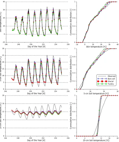
G0. The explanation for this discrepancy is found through the analysis of the measured and simulated temperatures of the soil profile. Although the measured dynamic temperature range is not entirely captured by the simulations, the modeled surface temperature and 5-cm soil temperature compare rea-sonably well with the measurements and results RMSD’s of 1.45–1.84 and 1.08–1.80◦C, respectively. On the other hand, the 25-cm soil temperature simulations strongly underesti-mate the measured diurnal temperature variation, which indi-cates that the heat required for the simulation of temperature variations deeper in the soil profile is not transferred into soil column. Since a relatively small amount of energy is used for heating the deeper soil profile, more energy is available for heating the atmosphere. Hence, the Noah overestimates theH.
Comparable results on the bias in partitioning theH and
[image:9.595.45.286.109.179.2]λE have previously been reported by Kahan et al. (2006). They have reported on over- and underestimations ofH and
Table 5. Root mean square difference (RMSD) calculated between
the measured soil temperature states and surface fluxes, and the Noah simulations.
Land cover H λE G0 Tskin T5cm T25cm
[W m−2] [W m−2] [W m−2] [◦C] [◦C] [◦C]
Tundra 53.50 32.40 34.12 1.48 1.08 1.19
Bare soil 57.85 42.54 33.34 1.84 1.80 1.77
Glacial 47.41 33.20 34.23 1.45 1.28 1.33
Table 6. Biases calculated between the measured soil temperatures
and surface fluxes, and the Noah simulations.
Land cover H λE G0 Tskin T5cm T25cm
[W m−2] [W m−2] [W m−2] [◦C] [◦C] [◦C]
Tundra −48.91 18.36 3.80 1.13 0.59 0.69
Bare soil −52.69 39.35 2.08 0.17 −0.24 0.28
Glacial −41.25 20.91 2.81 0.56 0.10 0.45
λEmeasured using SSiB at a Sahelian study site in Niger by as much as 31.2 and 41.8 W m−2, respectively. By reducing the model’s stomatal resistance (among other parameters) by more than one order of magnitude, theλEis increased and, because of the energy conservation principle, a reduction in
His enforced. The differences between the modeling results obtained with the three vegetation parameterizations should be viewed in this context. The smallest H overestimation is observed for the glacial vegetation parameterization. This parameterization includes a low value for minimum stom-atal resistance (Rc,min) and the lowest values for the rough-ness length for momentum transport (z0), which reduces the mechanically generated atmospheric turbulent fluxes. There-fore, Noah modeling results obtained through application of the “glacial” vegetation parameterization are considered to represent the Tibetan measurements best.
Also, the inconsistency of LSM’s in the simulation of the soil heat transfer has been previously recognized. Yang et al. (2005) extensively discussed the impact of the vertical heterogeneity in the soil profile for the simulation of the
[image:9.595.308.546.218.277.2]33 Fig. 4: Same as Fig. 3, except that the measured and simulated soil temperatures are shown for the surface and soil depths of 5-cm and 25-cm.
246 248 250 252 254 256
Day of the Year [#] -10
0 10 20 30 40
Sk
in
te
m
per
at
ur
e [
oC]
246 248 250 252 254 256
Day of the Year [#] 0
5 10 15 20 25 30
5-cm Soil te
m
pe
ratur
e [
oC]
246 248 250 252 254 256
Day of the Year [#] 0
4 8 12 16 20
25-cm So
il te
m
pe
ratu
re [
oC]
-10 0 10 20 30 40
Skin temperature [oC]
0 0.2 0.4 0.6 0.8 1
C
um
m
ul
at
iv
e di
st
ri
bu
ti
on
[
-]
0 10 20 30
5-cm Soil temperature [oC]
0 0.2 0.4 0.6 0.8 1
C
um
m
ulati
ve di
str
ibuti
on
[-]
0 4 8 12 16 20
25-cm Soil temperature [oC]
0 0.2 0.4 0.6 0.8 1
Cum
m
ulative
dis
tribution
[-]
Observed Bare soil Glacial Tundra
Fig. 4. Same as Fig. 3, except that the measured and simulated soil temperatures are shown for the surface and soil depths of 5-cm and
25-cm.
5 Optimizing Noah’s performance through adjustment of thermodynamic soil and vegetation parameteriza-tions
The analysis of the Noah modeling results obtained using default soil and vegetation parameterizations against in-situ measurements has shown that the transfer of heat through the soil column and the partitioning betweenH andλEare not properly simulated. In this section, the optimization of the simulation of these two land surface processes is inves-tigated by adjusting soil and vegetation parameterizations.
These adjustments include the evaluation of different numer-ical discretizations of the soil layers and calibration of soil and vegetation parameters.
Calibration of the soil and vegetation parameters is per-formed using the Parameter Estimation (PEST, Doherty 2003) tool, which is based on the optimization of a cost func-tion (8) using the Gauss-Levenberg Marquardt algorithm formulated by.
R. van der Velde et al.: Simulation of surface processes over a Tibetan plateau site 769
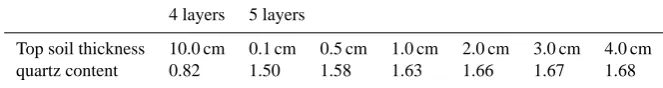
Table 7. Optimized values for qtz parameter using the PEST tool and the Noah LSM with seven numerical discretizations for the soil profile.
4 layers 5 layers
Top soil thickness 10.0 cm 0.1 cm 0.5 cm 1.0 cm 2.0 cm 3.0 cm 4.0 cm
quartz content 0.82 1.50 1.58 1.63 1.66 1.67 1.68
PEST allows users to assign weights to specific observations and different numerical schemes for the optimization of8. However, the objective of this investigation is to analyze the simulation of land surface processes over a Tibetan site by Noah and not to study different calibration strategies. For a complete mathematical description of PEST, the reader is re-ferred to Gallagher and Doherty (2007) and Doherty (2003). The default configuration of the PEST tool is used for this in-vestigation. To assure convergence, the optimization process has been performed for a wide range of initial parameter val-ues and during each optimization run only a single parameter is calibrated. A8based on the measured and simulatedG0 (8G0) is adopted for calibration of the STP and a8based on the measured and simulatedλE(8λE) is utilized to
cal-ibrate the vegetation parameters, independently. In this sec-tion, first, the influence of the soil parameterizations on the simulation of temperature states and surface energy balance is discussed and, then, the impact of the vegetation parame-ters is addressed.
5.1 Soil heat transfer
Since the large number of roots and the higher organic mat-ter content in the top soil changes thermal characmat-teristics as compared to the subsoil, the Noah is adapted to accommo-date different soil thermal layers (STL’s). In terms of STL’s, a 10-cm topsoil layer and 190-cm subsoil layer has been se-lected for this investigation. For the subsoil the default pa-rameterization for the thermal conductivity (κh) and heat
ca-pacitiy (C) have been assigned, while for the top soil aCsoil values of 1.0·106J m−3K−1 is taken and the qtz parameter in the κh parameterization is optimized by minimizing the 8G0. Within this calibration procedure, the upper and lower
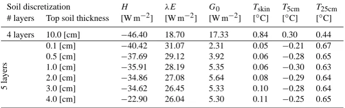
limits of the quartz content are set to 0.01 and 2.0 beyond values that are physically possible in order to maintain maxi-mum flexibility in the modeling system. In addition, different numerical discretizations of the soil profile are evaluated, of which the default 4-soil layer and six alternate 5-soil layer models are included. Within the 5-layer model setups, thick-nesses for the top soil layers of 0.1, 0.5, 1.0, 2.0, 3.0 and 4.0 cm have been selected, while maintaining the total thick-ness of the top two soil layers 10 cm.
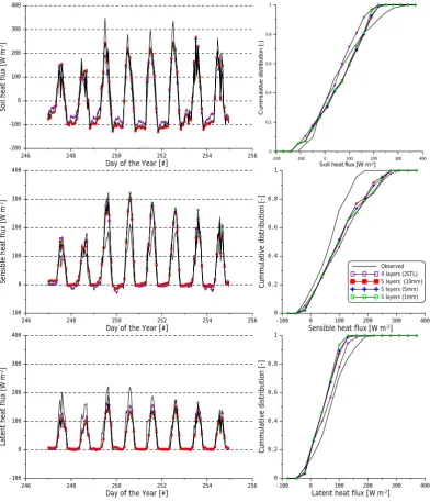
The qtz parameter is calibrated for all seven soil profile discretizations and the optimized values are presented in Ta-ble 7. The “glacial” vegetation parameterization has been used for these simulations. The modeled and measured sur-face fluxes are presented in Fig. 5 as time series as well as
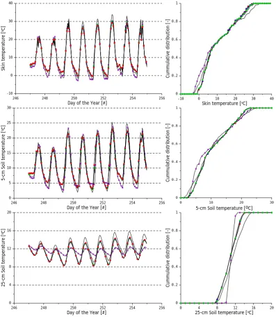
cumulative distributions. Similar plots are presented in Fig. 6 for the modeled and measured soil temperature at the surface and soil depths of 5 and 25-cm. The RMSD’s and biases be-tween modeling results and measurements of the heat fluxes and soil temperatures are given in Tables 8 and 9, respec-tively. It should be noted that the results of the Noah simu-lations using the 5-layer model setup with thicknesses of the top soil of 2.0, 3.0 and 4.0 cm are not shown in Figs. 5 and 6. The results presented in Figs. 5 and 6, and Tables 8 and 9 demonstrate that differentiation between the STP of the top-and subsoil alone improves the simulation of the soil tem-peratures only slightly and even increases the differences be-tween the simulated and measured surface fluxes. The sim-ulation of the soil heat transfer significantly improves when an additional thin soil layer is included in the model con-figuration. For all six thicknesses of the top soil layer, the largest improvements are observed in the simulation of the soil temperature at a depth of 25-cm (T25cm). The RMSD for theT25cm(RMSDT25cm)decreases from 1.33◦C obtained with the “glacial” vegetation parameterization and the de-fault numerical soil discretizations to values varying between 0.71 and 0.66◦C depending on the thickness of the top soil layer, which is a reduction of 46.6–50.3%. Also, the RMSD’s for simulated surface temperature (Tskin) and 5-cm soil tem-perature (T5cm) obtained with the 5-layer model setups de-crease as compared to the model results obtained with the default 4-layer configuration. TheTskinRMSD (RMSDTskin) decreases from 1.45◦C to values of 1.15–1.35◦C and for the T5cm RMSD (RMSDT5cm) a decrease from 1.28◦C to 1.02–1.11◦C is observed. Both the RMSDTskin as well as RMSDT5cmdepend on the thickness of the top soil layer; the lowest RMSDTskin and RMSDT5cm for a 0.1 cm top layer, while the lowest RMSDT25cm is obtained for a 1.0 cm top layer.
The impact of the adjustments in soil parameterization on the simulation of the surface energy balance is primar-ily manifested in theH andG0. Its influence on the simu-lation of theλEis limited and resulting RMSD (RMSDλE)
34 Fig. 5: Comparison of the heat fluxes measured and simulated using Noah with two soil thermal layers and different numerical discretizations of the soil profile. For reference also modeling results obtained with the default parameterizations are shown. The plots on the left side present the measurements and simulations as a time series, the right side plots show cumulative distributions.
246 248 250 252 254 256
Day of the Year [#]
-200 -100 0 100 200 300 400
Soil
hea
t fl
ux [W
m
-2]
246 248 250 252 254 256
Day of the Year [#]
-100 0 100 200 300 400
Se
nsible h
eat flux [W
m
-2]
246 248 250 252 254 256
Day of the Year [#]
-100 0 100 200 300 400
Latent heat
flux [W
m
-2]
-200 -100 0 100 200 300 400
Soil heat flux [W m-2] 0
0.2 0.4 0.6 0.8 1
C
u
m
m
ulat
ive dist
ri
buti
on [
-]
-100 0 100 200 300 400
Sensible heat flux [W m-2]
0 0.2 0.4 0.6 0.8 1
Cummulativ
e di
st
rib
utio
n [-]
-100 0 100 200 300 400
Latent heat flux [W m-2]
0 0.2 0.4 0.6 0.8 1
Cummulativ
e di
st
rib
utio
n [-]
[image:12.595.102.495.64.522.2]Observed 4 layers (2STL) 5 layers (10mm) 5 layers (5mm) 5 layers (1mm)
Fig. 5. Comparison of the heat fluxes measured and simulated using Noah with two soil thermal layers and different numerical discretizations
of the soil profile. For reference also modeling results obtained with the default parameterizations are shown. The plots on the left side present the measurements and simulations as a time series, the right side plots show cumulative distributions.
model with a 0.1-mm top layer (33.17 W m−2)because using the configuration diurnal temperature variations at the sur-face and at a 5-cm soil depth are simulated best. However, the change in the simulated surface temperature modifies also the temperature gradient between the skin and air. As a re-sult, an increase of RMSD forH (RMSDH) is observed as
the RMSDG0decreases, and vice versa. The lowest RMSDH
is obtained for the 5-layer model configuration using 4.0-cm top layer, which is 35.87 W m−2. The decrease in RMSDH
observed for thicker top layer in 5-layer model configuration is coupled with a decrease in the obtained bias, which range
from 40.42 to 22.9 W m−2 for top soil layer thicknesses of 0.1–4.0-cm. This indicates an improvement in the simula-tion of the heat flux partisimula-tioning, while even the lowest bias obtained for theH as well asλE remain quite significant; 22.90 and 26.04 W m−2, respectively.
R. van der Velde et al.: Simulation of surface processes over a Tibetan plateau site 771
35 Fig. 6: Same as Fig. 5, except that the measured and simulated soil temperatures are shown for the surface and soil depth of 5-cm and 25-cm.
246 248 250 252 254 256
Day of the Year [#]
-10 0 10 20 30 40
Sk
in tempe
ratu
re [
oC]
246 248 250 252 254 256
Day of the Year [#]
0 4 8 12 16 20
25
-c
m S
oi
l t
emp
er
atu
re [
oC]
246 248 250 252 254 256
Day of the Year [#]
0 5 10 15 20 25 30
5-cm
So
il t
em
pe
ratu
re [
oC]
-10 0 10 20 30 40
Skin temperature [oC]
0 0.2 0.4 0.6 0.8 1
Cummu
lati
ve di
st
rib
ution [-]
0 10 20 30
5-cm Soil temperature [oC]
0 0.2 0.4 0.6 0.8 1
Cu
mmu
la
ti
ve d
is
tr
ibuti
on [-]
0 4 8 12 16 20
25-cm Soil temperature [oC]
0 0.2 0.4 0.6 0.8 1
Cu
mm
ul
ati
ve
d
ist
ribu
[image:13.595.100.498.62.519.2]tion [-]
Fig. 6. Same as Fig. 5, except that the measured and simulated soil temperatures are shown for the surface and soil depth of 5-cm and 25-cm.
the measurements best, while differences between the mea-sured and simulatedH are smallest using a 4.0-cm top soil layer. The overestimation of theHwith 0.1-cm top soil layer might suggest that the simulated solar radiation available for heating of the air and soil is too large; meaning that the sim-ulated solar radiation consumed by the cooling of surface through evaporation and transpiration is too low. Further, it should be noted that the optimized values for the quartz con-tent for the all 5-layer model configurations exceed its physi-cal limits varying between 1.50 and 1.68. An explanation for these unrealistic values will be provided in the discussion.
5.2 Vegetation parameterization
Table 8. RMSD’s calculated between the measured soil temperature states and surface fluxes, and modelling results obtained with Noah
configured to accommodate different STP for the top- and subsoil and different numerical discretizations of the soil profile.
Soil discretization H λE G0 Tskin T5cm T25cm
# layers Top soil thickness [W m−2] [W m−2] [W m−2] [◦C] [◦C] [◦C]
4 layers 10.0 [cm] 52.72 33.17 41.28 1.40 1.49 1.32
5
layers
0.1 [cm] 46.92 37.04 33.17 1.15 1.02 0.71
0.5 [cm] 44.34 36.21 34.73 1.25 1.05 0.68
1.0 [cm] 43.30 36.13 36.83 1.32 1.07 0.66
2.0 [cm] 43.24 36.06 39.34 1.36 1.09 0.66
3.0 [cm] 43.51 35.97 40.47 1.35 1.11 0.67
4.0 [cm] 35.87 35.89 40.68 1.35 1.03 0.67
Table 9. Same as Table 8, except the biases are presented.
Soil discretization H λE G0 Tskin T5cm T25cm
# layers Top soil thickness [W m−2] [W m−2] [W m−2] [◦C] [◦C] [◦C]
4 layers 10.0 [cm] −46.40 18.70 17.33 0.84 0.30 0.44
5
layers
0.1 [cm] −40.42 31.07 2.31 0.05 −0.21 0.67
0.5 [cm] −37.69 29.12 3.92 0.06 −0.28 0.65
1.0 [cm] −35.91 28.19 5.35 0.06 −0.30 0.63
2.0 [cm] −34.86 27.08 5.64 0.08 −0.29 0.64
3.0 [cm] −34.62 26.45 5.33 0.10 −0.28 0.64
4.0 [cm] −22.90 26.04 5.30 0.11 −0.25 0.65
transpiration (Topt), currently fixed at a value of 24.85◦C, may need to be tuned to represent the Tibetan conditions.
Ideally, theRc,min andToptwould be obtained from long term data sets as has been done by Gimanov et al. (2008). This reaches, however, beyond our objective to identify the adjustments in soil and vegetation parameterization needed to improve Noah’s performance over the selected Tibetan site for a short 7-day period. Therefore, the parametersRc,min andToptare calibrated by minimizing the cost function be-tween the measured and simulatedλE. For this optimization procedure, the 5-layer Noah model configuration is used with a 0.5 cm top soil layer and a qtz value of 1.58. The calibration of theRc,minandToptyields values of 49.88 s m−1and 7.21 ◦C, respectively. Through the optimization, theR
c,minis re-duced by 100.12 s m−1andToptby 17.61◦C in comparison to the default parameterization. Both changes to the two plant physiological parameters can be argued. Growing seasons on the plateau are short and, in this short period, vegetation should be productive in order to be able to survive the harsh Tibetan environment. Further, temperatures on the plateau are, generally, lower than at sea level; a lower temperature at which plants transpire optimally is, therefore, required. At the same time, the validity of the defaultTopt can be ques-tioned for all environments that substantially differ from the humid climate for the original parameterization (Dickinson, 1984). A climate dependent parameterization could be con-sidered for global Noah applications, but this extends beyond the scope of this investigation.
The modeling results of Noah simulations with the op-timized vegetation parameters are plotted against measure-ments, which are presented in Figs. 7 and 8 for the heat fluxes and soil temperatures, respectively. For comparison purposes, a selection of Noah simulations discussed previ-ously are also presented in Figs. 7 and 8, which are; (1) the default 4-layer model with the “glacial” vegetation param-eters; (2) the 4-layer model with two STL’s and “glacial” vegetation parameters; and (3) the 5-layer model with two STL’s, 0.5-cm top layer and “glacial” vegetation parameters. In addition, the basic statistics are presented in the plots, such the coefficient of determination (R2), RMSD and bias.
[image:14.595.120.473.249.360.2]R. van der Velde et al.: Simulation of surface processes over a Tibetan plateau site 773
36
Fig. 7: Scatter plots of surface fluxes (
G 0, H , λ E ) m
easured and sim
ulated using Noah in its 1)
default configuration; 2) default num
erical disc
retizations of the soil profile and 2 STL’s; 3)
5-layer m
odel setup, 2 STL’s and top layer of
0.5 c
m
; 4) s
am
e as 3) e
xcept the vegetation
param eters a re ca libr ated . .
1:1 l ine -200 -100 0 100 200 300 400
Measured G0 [W m-2]
-200 -100 0 100 200 300 400 Sim ulated G 0 [W m -2]
-200 -100 0 100 200 300 400 Measured G0 [W m-2]
-200 -100 0 100 200 300 400 Sim ulated G 0 [W m -2]
-200 -100 0 100 200 300 400 Measured G0 [W m-2]
-200 -100 0 100 200 300 400 Sim ulated G 0 [W m -2]
-200 -100 0 100 200 300 400 Measured G0 [W m-2]
-200 -100 0 100 200 300 400 Sim ulated G 0 [W m -2]
-100 0 100 200 300 400
Measured H [W m-2] -100 0 100 200 300 400 Si m ul at ed H [W m -2]
-100 0 100 200 300 400
Measured H [W m-2] -100 0 100 200 300 400 Si mulated H [ W m -2]
-100 0 100 200 300 400
Measured H [W m-2] -100 0 100 200 300 400 Si mulated H [ W m -2]
-100 0 100 200 300 400
Measured H [W m-2] -100 0 100 200 300 400 Si mulated H [ W m -2]
-100 0 100 200 300 400
Measured LE [W m-2]
-100 0 100 200 300 400 Sim
ulated LE [W
m
-2]
-100 0 100 200 300 400
Measured LE [W m-2]
-100 0 100 200 300 400 Sim
ulated LE [W
m
-2]
-100 0 100 200 300 400
Measured LE [W m-2]
-100 0 100 200 300 400 Sim
ulated LE [W
m
-2]
-100 0 100 200 300 400
Measured LE [W m-2]
-100 0 100 200 300 400 Sim
ulated LE [W
m -2] Soil h eat f lu x Se ns ible h eat fl ux Lat en t hea t fl ux
4 layers (1 STL) 4 layers (2 STL) 5 layers (5mm) 5 layers (opt. veg.
params)
BIAS = 46.4 [W m-2]
R2=0.82 R2=0.85
R2=0.85
BIAS = -37.6 [W m-2] BIAS = 20.8 [W m-2]
BIAS = -41.3 [W m-2]
R2=0.85
RMSD = 47.4 [W m-2] RMSD = 52.7 [W m-2] RMSD = 44.34 [W m-2] RMSD = 33.3[W m-2]
BIAS = 18.7 [W m-2]
R2=0.69 R2=0.74
R2=0.67
BIAS = 29.1 [W m-2] BIAS = 20.8 [W m-2]
BIAS = 20.9 [W m-2]
R2=0.67
RMSD = 33.2 [W m-2] RMSD = 33.2 [W m-2] RMSD = 36.2 [W m-2] RMSD = 26.5[W m-2]
BIAS = 17.3 [W m-2]
R2=0.69 R2=0.74
R2=0.67
BIAS = 3.9 [W m-2]
BIAS = 2.8[W m-2]
R2=0.67
RMSD = 34.2 [W m-2] RMSD = 41.3 [W m-2] RMSD = 34.7 [W m-2] RMSD = 32.5[W m-2]
[image:15.595.74.522.65.395.2]BIAS = -0.3 [W m-2]
Fig. 7. Scatter plots of surface fluxes (G0,H,λE) measured and simulated using Noah in its (1) default configuration; (2) default numerical
discretizations of the soil profile and 2 STL’s; (3) 5-layer model setup, 2 STL’s and top layer of 0.5 cm; (4) same as (3) except the vegetation parameters are calibrated.
6 Discussion
The adjustments in the parameterization of the STP and cal-ibration of the vegetation parameters,Rc,minandTopt, have ameliorated the simulation of the soil heat transfer and re-duced uncertainties in the simulated H and λE to levels comparable as are reported in previous investigations (e.g., Sridhar et al., 2003; Gutmann and Small, 2007; and Pauwels et al., 2008). Despite the optimized Noah simulations are able to represent the soil temperature and surface energy bal-ance measurements better, still some inconsistencies in the modeling results can be observed when radiative forcings become large. For example, Noah systematically overesti-mates the measuredH at values larger than approximately 150 W m−2, which coincides with underestimation of theG0 andTskinwhen the measured values are larger than approx-imately 150 W m−2and 20◦C, respectively. Apparently, un-der large radiative forcings Noah is not able to simulateTskin increase measured on the Tibetan Plateau. Therefore, the simulated temperature gradients between the surface and at-mosphere, and between surface and the mid-point of the first
soil layer become too large and too small, respectively. As a result, an over- and underestimation of the measuredH and
G0are observed. The explanation of this discrepancy in the simulatedTskinis twofold.
First, the surface exchange coefficient for heat (Ch) may
not be properly parameterized for the Tibetan conditions. Noah uses the Reynolds number dependent method pro-posed by Zilintinkevich (1995) to determine the kB−1. How-ever, Yang et al. (2008) showed for bare soil surfaces that Reynolds number dependent kB−1methods, in general, tend to underestimate the strong diurnal kB−1variations observed over the Tibetan Plateau (e.g. Ma et al. 2005 and Yang et al. 2003). A kB−1underestimation during daytime results in more efficient heat transfer between the soil surface and the atmosphere, which causes anH overestimation and ex-plains also the discrepancy between the measured and sim-ulatedTskin. Other kB−1methods (e.g. Su et al. 2001 and
37
e as Fig. 7 ex
pect th
at th
e tem
perature states (
T ski n, T 5cm and T 25cm
) are shown here.
0 5 10 15 20
Measured T25cm [oC]
0 5 10 15 20 Simu la te d T 25 cm [ oC]
1:1 l ine
-10 0 10 20 30 40
Measured Tskin [oC]
-10 0 10 20 30 40 Si m ul at ed T sk in [ oC]
-10 0 10 20 30 40
Measured Tskin [oC]
-10 0 10 20 30 40 Si m ul at ed T sk in [ oC]
-10 0 10 20 30 40
Measured Tskin [oC]
-10 0 10 20 30 40 Si m ul at ed T sk in [ oC]
-10 0 10 20 30 40
Measured Tskin [oC]
-10 0 10 20 30 40 Si m ul at ed T sk in [ oC]
0 5 10 15 20 25 30
Measured T5cm [oC]
0 5 10 15 20 25 30 Sim ulate d T 5c m [ oC]
0 5 10 15 20 25 30
Measured T5cm [oC]
0 5 10 15 20 25 30 Sim ulate d T 5c m [ oC]
0 5 10 15 20 25 30
Measured T5cm [oC]
0 5 10 15 20 25 30 Sim ulate d T 5c m [ oC]
0 5 10 15 20 25 30
Measured T5cm [oC]
0 5 10 15 20 25 30 Sim ulate d T 5c m [ oC]
0 5 10 15 20
Measured T25cm [oC]
0 5 10 15 20 Si m ul ated T25 cm [ oC]
0 5 10 15 20
Measured T25cm [oC]
0 5 10 15 20 Si m ul ated T25 cm [ oC]
0 5 10 15 20
Measured T25cm [oC]
0 5 10 15 20 Si m ul ated T25 cm [ oC] Sk in T em per at ur e 5-cm s oil t emp er at ur e 25 -c m so il tem pe rat ur e
4 layers (1 STL) 4 layers (2 STL) 5 layers (5mm) 5 layers (opt. veg.
params)
BIAS = 0.30 [oC]
R2=0.98 R2=0.95
R2=0.92
BIAS = -0.28 [oC] BIAS = 1.17 [oC]
BIAS = 0.10 [oC]
R2=0.88
RMSD = 1.28 [oC] RMSD = 1.49 [oC] RMSD = 1.05 [oC] RMSD = 1.17 [oC]
BIAS = 0.44 [oC]
R2=0.95 R2=0.90
R2=0.55
BIAS = 0.65 [oC] BIAS = 1.09 [oC]
BIAS = 0.45 [oC]
R2=0.51
RMSD = 1.33 [oC] RMSD = 1.32 [oC] RMSD = 0.68 [oC] RMSD =1.10 [oC]
BIAS = 0.84 [oC]
R2=0.99 R2=0.99
R2=0.98
BIAS = 0.06 [oC]
BIAS = 0.56 [oC]
R2=0.98
RMSD = 1.45 [oC] RMSD = 1.40 [oC] RMSD = 1.25 [oC] RMSD = 1.43 [oC]
BIAS = 1.49 [oC]
Fig. 8. Same as Fig. 7 expect that the temperature states (Tskin,T5cmandT25cm)are shown here.
kB−1 methods readers are referred to Liu et al. (2007) and Yang et al. (2008).
Second, the linearization of the surface energy balance (see Eq. (10)) utilized to compute the Tskin contributes to explaining the differences between the simulated and mea-suredTskin. This approximation is exact whenTairis equiv-alent toTskinand loses its validity as the difference between
Tair andTskin increases. For our Tibetan study site, differ-ences between theTairandTskin can be expected to be sig-nificantly larger than at sea level because the air pressure is much lower and fewer air molecules are available to transport energy from the surface towards the air. To demonstrate the impact of the applied approximation for our Tibetan site, the measuredTskinandTair, theTskincalculated by using Eq. (10) and are plotted in Fig. 9. This plot shows that the applied ap-proximation holds rather well during nighttime. After sun-rise, however, differences between measuredTair andTskin increase resulting in a discrepancy between the measured and approximatedTskinof more than 10◦C at midday. Obviously, this leads to an underestimation ofTskin even when the pa-rameterization of the soil-vegetation-atmosphere system is agreement with the local conditions.
Within the uncertainties embedded in theCh calculation
and in the linearization applied for theTskin simulation lies also the explanation for the unrealistically high values of the calibrated qtz parameter. With the increase of the qtz param-eter, the thermal heat conductance is raised to increase the transport of heat into soil and to compensate for the lower simulated temperature gradient between surface and the mid point of the first soil layer. When the qtz parameter is not used to compensate for theTskinunderestimation, biases arise in the simulation of the soil temperature profile as occurs in Noah applications in the default configuration.
[image:16.595.74.522.64.403.2]R. van der Velde et al.: Simulation of surface processes over a Tibetan plateau site 775
[image:17.595.129.470.64.257.2]38 Fig. 9: Measurements of the air and surface temperature, and the surface temperature approximated using Eq. 10 plotted as a time series for the analyzed period of meteorological forcing collected at a Tibetan Plateau site.
246 248 250 252 254 256
Day of the Year [#]
-10 0 10 20 30 40
Temperature [
oC]
Air temperature Measured Tsk Approximated Tsk
Fig. 9. Measurements of the air and surface temperature, and the surface temperature approximated using Eq. (10) plotted as a time series
for the analyzed period of meteorological forcing collected at a Tibetan Plateau site.
of the 5-layer configuration closer to a value that is realisti-cally possible, but is still far too high.
Using the qtz value of 1.45 and 5-layer discretization with a 0.5 cm top layer, the vegetation parameters,Rc,minandTopt, have also been recalibrated with a LAI of 1.2 m2m−2, which results in values of 20.89 s m−1 and 9.73◦C, respectively. Compared to the vegetation parameter presented above, the
Rc,min has decreased by more than a factor two, while the Topt has increased only slightly. This large reduction in
Rc,min follows directly from Eq. (24), in which the Rc,min and LAI have an opposite effect on the calculation of theRc.
Thus, the decrease in LAI is for a large part compensated within the model calibration by decreasing theRc,min.
As to determine whether using the MODIS LAI improves Noah’s performance, RMSD values between the measured and simulated soil temperatures and heat fluxes have been computed for the three additional Noah simulations and are presented in Table 10. Comparison of the RMSD values of Table 10 with the results presented previously shows that the simulation of the temperatures across the soil profile im-proves somewhat. However, Noah’s overall ability to simu-late the heat fluxes decreases when using the MODIS LAI. Apparently, Noah has been tuned to perform optimally using LAI of 5.0 m2m−2, which is probably the reason for using a fixed value for large-scale Noah applications.
7 Conclusions
[image:17.595.309.545.428.487.2]In this paper, adjustments in the soil and vegetation param-eterizations required to be able to reproduce the soil tem-perature states and surface fluxes using the Noah LSM are investigated using a 7-day period of in-situ measurements collected at a study site on the Tibetan Plateau. Analysis
Table 10. RMSD values calculated between soil temperatures and
surface fluxes measured and simulated by Noah using a LAI value
of 1.2 m2m−2; 4-layer∼Noah simulations obtained with the
de-fault 4 layer soil discretization and calibrating the qtz parameter
(=0.66); 5-layer∼ Noah simulation obtained using 5 layers (top
layer=0.5 cm) and calibrating the qtz parameter (=1.45); 5l+veg∼
Noah simulations obtained 5-layer soil discretization and qtz
pa-rameter and calibrating the vegetation papa-rametersRc,minandTopt
(20.89 s m−1and 9.73◦C).
H λE G0 Tskin T5cm T25cm
[W m−2] [W m−2] [W m−2] [◦C] [◦C] [◦C]
4 layer 67.29 43.46 38.64 1.48 1.08 1.19
5 layer 58.74 50.92 35.81 0.97 1.04 0.51
5l+veg. 35.41 26.85 33.78 1.33 1.18 1.09
of the results from simulations obtained through application of the default parameterization has shown that (1) heat trans-fer through the soil column is not represented adequately, (2) partitioning between the sensible (H) and latent heat (λE) flux is biased. Amelioration of the parameterization of these land surface processes is achieved through adjustment of soil and vegetation parameterizations.
Through differentiating between the soil thermal proper-ties of a top- and subsoil, and including a thin top soil layer, uncertainties in the simulation of the soil heat transfer are reduced and RMSD’s between the measured and simulated
Tskin, T5cm andT25cm are obtained of 1.25◦C, 1.05◦C and 0.68◦C by using a 0.5 cm thick top soil layer. It is found that adding a thin top soil layer has stronger effect than differ-entiating between the soil thermal properties of a top- and subsoil. A decrease in the vegetation parameters,Rc,minand
λEfrom 33.2 W m−2obtained using the default Noah con-figuration to 26.5 W m−2using the optimized parameteriza-tion. In addition, the improvement in theλEsimulation also influences theH simulation and decreases the RMSD from 47.41 to 33.3 W m−2, while the differences between the mea-sured and simulatedG0do not change significantly.
Although the adjustments in the parameterization of the STP and calibration of vegetation parameters improved Noah’s capability of representing the soil temperature states and the surface energy balance components measured on the Tibetan Plateau, under conditions of the high radiative forcings an underestimation is observed of measuredTskin. This underestimation of theTskinresults in an overestimation of theH and underestimationG0. The explanation for the discrepancy in the Tskin simulation is twofold. First, the surface exchange coefficient for heat may not be properly parameterized. Second, the approximation, adopted for linearization of the surface energy balance for the Tskin calculation, introduces some uncertainties when differences between the measured Tskin and Tair are large, which are typical midday conditions on the Tibetan Plateau.
Edited by: J. Wen
References
Chen, F., Janjic, Z., and Mitchell, K.: Impact of atmospheric surface-layer parameterizations in the new land-surface scheme of the NCEP mesoscale ETA model, Bound.-Lay. Meteorol., 85, 391–421, 1997.
Cosby, B. J., Hornberger, G. M., Clapp, R. B., and Ginn, T. R.: Water Resour. Res., 20, 682-690, 1984.
Dickinson, R. E.: Modeling evapotranspiration for
three-dimensional global climate models, in: Climate processes and climate sensitivity, editedy by: Hansen, J. E. and Takahashi, T., American Geophysical Union, Geophys. Monogr., 29, 58–72, 1984.
Dickinson, R. E., Oleson, K. W., Bonan, G., Hoffman, F., Thornton, P., Vertenstein, M., Yang, Z.-L., and Zeng, X.: The community land model and its climate statistics as a component of the com-munity climate system model, J. Climate, 19, 2302–2324, 2006. Doherty, J.: Manual for the PEST Surface Water Modelling Util-ities, Watermark Numerical Computing, Australia, available at http://www.sspa.com/pest, 2003.
Duan, Q., Schaake, J., Andr´eassian, V., et al.: Model parameter es-timation experiment (MOPEX): An overview of science strategy and major results from the second and third workshops, J. Hy-drol., 320, 3–17, 2006.
Ek, M. B., Mitchell, K. E., Lin, Y., Rogers, E., Grunmann, P., Ko-ren, V., Gayno, G., and Tarpley, J. D.: Implementation of Noah land surface model advances in the National Centers for Environ-mental Prediction operational mesoscale Eta model, J. Geophys. Res., 108, 8851, doi:10.1029/2002JD003296, 2003.
Gallagher, M. and Doherty, J.: Parameter estimation and uncer-tainty analysis for a watershed model, Environ. Modell. Softw., 22, 1000–1020, 2007.
Garratt, J. R.: Sensitivity of climate simulations to land-surface and atmospheric boundary-layer treatments – A review, J. Climate, 6, 419-448, 1993.
Gilmanov, T. G., Soussana, J. F., Aires, L., et al.: Partitioning
Euro-pean grassland net ecosystem CO2exchange into gross primary
productivity and ecosystem respiration using light response func-tion analysis, Agr. Ecosyst. Environ., 121, 93–120, 2007. Gutmann, E. D. and Small, E. E.: A comparison of land surface
model soil hydraulic properties estimated by inverse modeling and pedotransfer functions, Water Resour. Res., 43, W05418, doi:10.1029/2006WR005135, 2007.
Gulden, L. E., Rosero, E., Yang, Z., Rodell, M., Jackson, C. S., Niu, G., Yeh, P. J.-F., and Famiglietti, J.: Improving land-surface model hydrology: Is an explicit aquifer model better than a deeper soil profile?, Geophys. Res. Lett., 34, L09402, doi:10.1029/2007GL029804, 2007.
Hillel, D.: Environmental soil physics, Academic Press, 771 pp., 1998.
Hogue, T. S., Bastidas, L., Gupta, H., Sorooshian, S., Mitchell, K., and Emmerich, W.: Evaluation and transferability of the Noah land surface model in semiarid environments, J. Hydrometeorol., 6, 68–83, 2005.
International GEWEX Project Office: GSWP-2: The Second
Global Soil Wetness Project Science and Implementation Plan. IGPO Publication Series No. 37, 65 pp., 2002.
Jacquemin, B. and Noilhan, J.: Sensitivity study and validation of a land surface parameterization using the HAPEX-MOBILHY data set, Bound.-Lay. Meteorol., 52, 93–134, 1990.
Jarvis, P. G.: The interpretation of the variations in leaf water po-tential and stomatal conductance found in canopies in the field, Philos. T. Roy. Soc. B, 273, 593–610, 1976.
Johansen, O.: Thermal conductivity of soils. Ph.D thesis, University of Trondheim, 236 pp., 1975.
Kahan, D. S., Xue, Y., and Allen S. J.: The impact of vegetation and soil parameters in simulations of surface energy and water balance in the semi-arid sahel: A case study using SEBX and HAPEX-Sahel data, J. Hydrol., 320, 238–259, 2006.
Kato, H., Rodell, M., Beyrich, F., Cleugh, H., van Gorsel, E., Liu, H., and Meyers, T. P.: Sensitivity of land surface simulations to model physics, land characteristics, and forcings, at four CEOP Sites, J. Meteorol. Soc. Jpn., 87A, 187–204, 2007.
Kersten, M. S.: Thermal properties of soils. University of Min-nesota Engineering Experiment Station Bulletin 28, 227 pp., available from University of Minnesota Agricultural Experiment Station, St. Paul, MN 55108, 1949.
Koster, R. D., Dirmeyer, P. A., Guo, Z., et al.: Regions of strong coupling between soil moisture and precipitation, Science, 305, 1138–1140, 2004.
Liu, S., Lu, L., Mao, D., and Jia, L.: Evaluating parameterizations of aerodynamic resistance to heat transfer using field measure-ments, Hydrol. Earth Syst. Sci., 11, 769–783, 2007,
http://www.hydrol-earth-syst-sci.net/11/769/2007/.