https://doi.org/10.5194/hess-23-1103-2019 © Author(s) 2019. This work is distributed under the Creative Commons Attribution 4.0 License.
Technical note: Analytical sensitivity analysis and uncertainty
estimation of baseflow index calculated by a two-component
hydrograph separation method with conductivity as a tracer
Weifei Yang1,2,3, Changlai Xiao1,2,3, and Xiujuan Liang1,2,3
1Key Laboratory of Groundwater Resources and Environment, Ministry of Education, No. 2519, Jiefang Road, Changchun 130021, PR China
2National-Local Joint Engineering Laboratory of In-situ Conversion, Drilling and Exploitation Technology for Oil Shale, No. 2519, Jiefang Road, Changchun 130021, PR China
3College of New Energy and Environment, Jilin University, No. 2519, Jiefang Road, Changchun 130021, PR China Correspondence:Changlai Xiao ([email protected])
Received: 16 September 2018 – Discussion started: 11 October 2018
Revised: 26 January 2019 – Accepted: 5 February 2019 – Published: 25 February 2019
Abstract. The two-component hydrograph separation method with conductivity as a tracer is favored by hydrolo-gists owing to its low cost and easy application. This study analyzes the sensitivity of the baseflow index (BFI, long-term ratio of baseflow to streamflow) calculated using this method to errors or uncertainties in two parameters (BFC, the conductivity of baseflow, and ROC, the conductivity of surface runoff) and two variables (yk, streamflow, and SCk,
specific conductance of streamflow, where k is the time step) and then estimates the uncertainty in BFI. The analysis shows that for time series longer than 365 days, random measurement errors inykor SCk will cancel each other out,
and their influence on BFI can be neglected. An uncertainty estimation method of BFI is derived on the basis of the sensitivity analysis. Representative sensitivity indices (the ratio of the relative error in BFI to that of BFCor ROC) and BFI0 uncertainties are determined by applying the resulting equations to 24 watersheds in the US. These dimensionless sensitivity indices can well express the propagation of errors or uncertainties in BFCor ROCinto BFI. The results indicate that BFI is more sensitive to BFC, and the conductivity two-component hydrograph separation method may be more suitable for the long time series in a small watershed. When the mutual offset of the measurement errors in conductivity and streamflow is considered, the uncertainty in BFI is reduced by half.
1 Introduction
Hydrograph separation (also called baseflow separation), aims to identify the proportion of water in different runoff pathways in the export flow of a basin, which helps in iden-tifying the conversion relationship between groundwater and surface water; in addition, it is a necessary condition for op-timal allocation of water resources (Cartwright et al., 2014; Miller et al., 2014; Costelloe et al., 2015). Some researchers indicated that tracer-based hydrograph separation methods yield the most realistic results because they are the most physically based methods (Miller et al., 2014; Mei and Anag-nostou, 2015; Zhang et al., 2017). Many hydrologists have suggested that electrical conductivity can be used as a tracer in hydrograph separation (Stewart et al., 2007; Munyaneza et al., 2012; Cartwright et al., 2014; Lott and Stewart, 2016; Okello et al., 2018). Conductivity is a suitable tracer because its measurement is simple and inexpensive, and it has distinct applicability in long-series hydrograph separation (Okello et al., 2018).
a. contributions from end-members other than baseflow and surface runoff are negligible;
b. the specific conductance of runoff and baseflow are con-stant (or vary in a known manner) over the period of record;
c. in-stream processes (such as evaporation) do not change specific conductance markedly;
d. baseflow and surface runoff have significantly different specific conductance.
bk=
yk(SCk−ROc)
BFc−ROc , (1)
wherebis baseflow (L3T−1),yis streamflow (L3T−1), SC is the electrical conductivity of streamflow, andk is time step number. The two parameters BFC and ROC represent the electrical conductivity of baseflow and surface runoff, re-spectively.
Stewart et al. (2007) conducted a field test in a drainage basin of 12 km2in southeast Hillsborough County, Florida, and showed that the maximum conductivity of streamflow can be used to replace BFCand the minimum conductivity can be used to replace ROC. However, Miller et al. (2014) pointed out that the maximum conductivity of streamflow may exceed the real BFC; therefore, they suggested that the 99th percentile of the conductivity of each year should be used as BFCto avoid the impact of high BFCestimates on the separation results and assumed that baseflow conductiv-ity varies linearly between years. The determination of the parameters (BFC, ROC) of the conductivity two-component hydrograph separation method involves some uncertainties (Miller et al., 2014; Okello et al., 2018). Therefore, sensi-tivity analysis of parameters and quantitative analysis of the uncertainties will contribute towards further optimization of the CMB method and improving the accuracy of hydrograph separation.
Most existing parameter sensitivity analysis methods are empirical methods that usually substitute varying values of a certain parameter into the separation model and then com-pare the range of the separation results produced by these varying parameter values (Eckhardt, 2005; Miller et al., 2014; Okello et al., 2018). Eckhardt (2012) indicated that “An empirical sensitivity analysis is only a makeshift if an analytical sensitivity analysis, that is an analytical calcula-tion of the error propagacalcula-tion through the model, is not feasi-ble”. Eckhardt (2012) derived sensitivity indices of equation parameters by the partial derivative of a two-parameter re-cursive digital baseflow separation filter equation. Until now, the parameters’ sensitivity indices of the CMB equation have not been derived.
At present, the uncertainty in the separation results of the CMB method is mainly estimated using an uncertainty trans-fer equation based on the uncertainty in BFC, ROC, and SCk
(Genereux, 1998; Miller et al., 2014). See Sect. 3.1 for de-tails. In this uncertainty estimation method, the uncertainty in the baseflow ratio (fbf, the ratio of baseflow to streamflow in a single calculation process) is estimated, and the average uncertainty in multiple calculation processes is then used to estimate the uncertainty in the baseflow index (BFI, long-term ratio of baseflow to total streamflow). This method can neither directly estimate the uncertainty in BFI nor consider the randomness and mutual offset of conductivity measure-ment errors, and, thus, it does not provide accurate estimates of BFI uncertainty.
The main objectives of this study are as follows: (i) ana-lyze the sensitivity of long-term series of baseflow separation results (BFI) to parameters and variables of the CMB equa-tion (Sect. 2); (ii) derive the uncertainty in BFI (Sect. 3). The derived solutions were applied to 24 basins in the US, and the parameter sensitivity indices and BFI uncertainty charac-teristics were analyzed (Sect. 4).
2 Sensitivity analysis
2.1 Parameters BFCand ROC
In order to calculate the sensitivity indices of the parameters, the partial derivatives ofbk in Eq. (1) with respect to BFC and ROCare required (the derivation process is expressed as Eqs. A1 and A2):
∂bk ∂BFc
= −yk
SCk−ROc
(BFc−ROc)2
, (2)
∂bk ∂ROc
=yk
SCk−BFc (BFc−ROc)2
. (3)
For the convenience of comparison, the baseflow index (BFI) is selected as the baseflow separation result for long time se-ries to analyze the influence of parameter uncertainty on BFI,
BFI=
n P k=1
bk
n P k=1
yk
=b
y, (4)
wherebandydenote the total baseflow and total streamflow, respectively, over the whole available streamflow sequences, andnis the number of available streamflow data.
Then, the partial derivatives of BFI to BFC and ROC should be calculated (the derivation process is presented in Eqs. A3 and A4):
∂BFI
∂BFc
=
yROc−
n P k=1
ykSCk
∂BFI
∂ROc =
n P
k=1
ykSCk−yBFc
y(BFc−ROc)2
. (6)
The definition of the partial derivative suggests that the in-fluence of the errors in the parameters (1BFCand1ROC) in Eq. (1) on the BFI can be expressed by the product of the er-rors and its partial derivatives. Then the erer-rors in BFI caused by small errors in BFCand ROCcan be approximated by
1BFcBFI= ∂BFI
∂BFc
1BFc=
yROc−
n P k=1
ykSCk
y(BFc−ROc)2
1BFc, (7)
1ROcBFI= ∂BFI
∂ROc1ROc=
n P
k=1
ykSCk−yBFc
y(BFc−ROc)2
1ROc. (8) The dimensionless sensitivity indices (S) can be obtained by comparing the relative error in BFI caused by the small errors in BFC and ROC with that of BFC and ROC (see Eqs. B1 and B2):
S (BFI|BFc)=1BFcBFI
BFI 1BF c BFc = BFc
yROc−
n P k=1
ykSCk
yBFI(BFc−ROc) 2
, (9)
S (BFI|ROc)=
1ROcBFI
BFI 1ROc ROc = ROc n P k=1
ykSCk−yBFc
yBFI(BFc−ROc) 2
, (10)
where S(BFI|BFc) represent the dimensionless sensitiv-ity index of BFI (output) with BFc (uncertain input) and
S(BFI|ROc)with ROc.
The dimensionless sensitivity index is also called the “elasticity index”, and it reflects the proportional relation-ship between the relative error in BFI and the relative error in parameters (e.g., ifS(BFI|BFc)=1.5 and the relative er-ror in BFcis 5 %, then the relative error in BFI is 1.5 times 5 %=7.5 %). After determining the values of BFC, ROC, BFI,y,yk, and SCk, the sensitivity indicesS(BFI|BFc)and S(BFI|ROc)can be calculated and compared.
2.2 Variablesykand SCk
In addition to the two parameters, there are two variables (SCkandyk) in Eq. (1). This section describes the sensitivity
analysis of BFI to these two variables. Similar to Sect. 2.1, the partial derivatives ofbk in Eq. (1) to SCk andyk are
ob-tained (see Eqs. A5 and A6), and the partial derivatives of BFI to SCkandykare further obtained (see Eqs. A7 and A8):
∂BFI
∂SCk
= 1
BFc−ROc, (11)
∂BFI ∂yk = n P k=1
(SCk−ROc)−nBFI(BFc−ROc) y (BFc−ROc)
. (12)
According to previous studies (Munyaneza et al., 2012; Cartwright et al., 2014; Miller et al., 2014; Okello et al., 2018) and this study (Table 1), the difference between BFC and ROC is often greater than 100 µs cm−1. Therefore,
∂BFI/∂SCk is usually less than 0.01 cm µs−1. Appendix C
shows that the value of∂BFI/∂yk is usually far less than
1 day m−3.
Small errors in SCk andyk cause errors in BFI: 1SCkBFI=
∂BFI
∂SCk
1SCk=
1SCk
BFc−ROc, (13)
1ykBFI=
∂BFI ∂yk 1yk = n P k=1
(SCk−ROc)−nBFI(BFc−ROc) y (BFc−ROc)
1yk. (14) The errors in BFI caused by SCk andyk are summed up to
obtain the error in BFI caused by
n P
k=1
SCk and n P
k=1
yk in the
whole time series:
1Pn
k=1SCkBFI=
n X
k=1
1SCkBFI=
n X
k=1
1SCk
BFc−ROc
= 1
BFc−ROc
n X
k=1
1SCk, (15)
1Pn
k=1ykBFI=
n X
k=1
1ykBFI=
n X k=1 , n P k=1
(SCk−ROc)−nBFI(BFc−ROc)
y (BFc−ROc)
1yk = n P k=1
(SCk−ROc)−nBFI(BFc−ROc) y (BFc−ROc)
n X
k=1
1yk. (16)
Wagner et al. (2006) reported that the uncertainty in instru-ments is usually less than 5 % for SCk (<100 µs cm−1) and
less than 3 % for SCk(>100 µs cm−1). According to
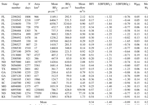
Table 1.Basic information, parameter sensitivity analysis, and uncertainty estimation results for 24 basins in the US. The asterisk in the “area” column indicates that the values are estimated based on data from adjacent sites.
State Gage N Area Mean ROC Mean BFI S(BFI|BFC) S(BFI|ROC) WBFI Mean
number days km2 BFC µs cm−1 baseflow Wfbf
µs cm−1 m3/s
FL 2298202 1808 966 1149.1 292.5 2.12 0.31 −1.32 −0.76 0.05 0.12
FL 2310545 1218 119∗ 6404.7 531.5 0.65 0.17 −1.11 −0.44 0.05 0.06
FL 2310650 779 77∗ 6558.7 3210.0 0.90 0.57 −1.84 −0.79 0.18 0.27
FL 2303000 728 570 432.7 120.5 2.32 0.34 −1.30 −0.77 0.06 0.14
FL 2298488 1303 76 737.3 194.0 0.14 0.38 −1.32 −0.58 0.14 0.18
FL 2298554 899 207∗ 969.2 320.5 0.50 0.30 −1.25 −1.22 0.13 0.27
FL 2298492 1478 16 1238.2 304.0 0.05 0.30 −1.11 −0.82 0.13 0.31
FL 2298495 330 10 1870.0 662.0 0.29 0.25 −1.52 −1.65 0.03 0.08
FL 2298527 807 23 1410.7 201.5 0.10 0.19 −1.03 −0.74 0.06 0.18
FL 2298530 1510 17 1460.8 348.0 0.14 0.29 −1.27 −0.77 0.08 0.13
FL 2297100 2979 342 1260.6 221.5 0.92 0.25 −1.18 −0.64 0.08 0.20
FL 2313000 787 4727 407.2 173.0 5.89 0.51 −1.71 −0.71 0.19 0.28
FL 2300500 821 386 447.9 83.0 0.30 0.20 −1.21 −0.89 0.05 0.11
ND 5057000 1401 16757 1420.6 610.0 2.08 0.51 −1.75 −0.74 0.14 0.21
ND 5056000 1277 5361 1681.4 546.0 3.61 0.44 −1.50 −0.60 0.07 0.14
TX 8068275 2801 482 361.7 65.0 0.57 0.15 −1.18 −1.23 0.06 0.11
GA 2336300 1235 225 230.4 63.0 0.79 0.31 −1.28 −0.88 0.16 0.33
GA 2207120 1383 417 312.5 59.0 1.48 0.24 −1.14 −0.76 0.09 0.20
SC 2160105 1363 1966 124.7 51.0 6.36 0.36 −1.56 −1.30 0.14 0.27
SC 2160700 1392 1150 148.7 51.0 4.45 0.37 −1.40 −0.94 0.15 0.28
MO 6894000 1375 477 1031.9 334.0 0.79 0.25 −1.40 −1.50 0.13 0.22
MO 6895500 802 1258481 786.7 428.0 939.98 0.57 −2.17 −0.90 0.06 0.20
ND 5082500 1274 77959 1390.6 427.0 77.19 0.38 −1.30 −0.77 0.15 0.26
KS 7144780 575 1847 1389.1 678.0 1.73 0.54 −1.73 −0.91 0.14 0.26
Mean 0.34 −1.40 −0.89 0.11 0.20
Standard deviation (SD) 0.13 0.28 0.29 0.05 0.08
considered to be ±5 %. The errors in SCk and yk mainly
comprise random measurement errors which mostly follow a normal distribution or a uniform distribution (Huang and Chen, 2011). Considering the mutual offset of random er-rors, when the time series (n) is sufficiently long,
n P k=1
1SCck
in Eq. (15) and
n P
k=1
1ykin Eq. (16) will approach zero.
The analysis of
n P k=1
1SCkand n P k=1
1ykunder different time series (n) and different error distributions (normal distribu-tion or uniform distribudistribu-tion) of a surface water stadistribu-tion (USGS site number 0297100) showed that the random errors in daily average conductivity and streamflow have a negligible effect on BFI when the time series is greater than 365 days (see Supplement S1 for detail).
3 Uncertainty estimation 3.1 Previous attempts
According to previous studies, in the case where a variableg
is calculated as a function of several factorx1,x2,x3, . . . ,xn (e.g.,g=G(x1,x2,x3, . . . ,xn)) and based on the assump-tions that the factors are uncorrelated and have a Gaussian distribution, the transfer equation (also known as Gaussian error propagation) between the uncertainty in the indepen-dent factors and the uncertainty ingis
Wg= s
∂g
∂x1
Wx1 2
+
∂g
∂x2
Wx2 2
+. . .+
∂g
∂xn Wxn
2
, (17) whereWg,Wx1,Wx2, andWxn are the same type of
uncer-tainty values (e.g., all average errors or all standard devia-tions) for g, x1, x2, and xn, respectively. A more detailed
description of this equation can be found in Taylor (1982), Kline (1985), and Ernest (2005).
byt values from the Student’st distribution (eacht for the same confidence level, such as 95 %) has the advantage of providing a clear meaning (tied to a confidence interval) for the computed uncertainty would correspond to, for example, 95 % confidence limits on BFI”.
Based on the above principle, Genereux (1998) substituted Eq. (18) into Eq. (17) to derive the uncertainty estimation equation (Eq. 19) of the CMB method:
fbf=
SCk−ROc BFc−ROc
, (18)
Wfbf=
s f
bf
BFc−ROc
WBFC
2 +
1−f bf
BFc−ROc
WROc
2 +
1
BFc−ROc
WSC 2
, (19) wherefbf is the ratio of baseflow to streamflow in a single calculation process,Wfbfis the uncertainty infbfat the 95 % confidence interval,WBFC andWROC are the standard devi-ations of the BFCand ROC multiplied by thet value (α= 0.05; two-tail) from the Student’s distribution, and WSC is the analytical error in conductivity multiplied by thet value (α=0.05; two-tail) (Miller et al., 2014).
Better estimates of the uncertainty in fbf within a single calculation step can be obtained using Eq. (19). Hydrologists usually approximate the uncertainty in BFI by averaging the uncertainty in all steps (Genereux, 1998; Miller et al., 2014). However, this method does not consider the mutual offset of the conductivity measurement errors and cannot accurately reflect the uncertainty in BFI. In this study, an uncertainty estimation equation of BFI is derived on the basis of the pa-rameter sensitivity analysis.
3.2 Uncertainty estimation of BFI
BFI is a function of BFc, ROc, SCk, andyk. In addition, the
uncertainties in BFc, ROc, SCk, andyk are independent of
each other. As explained earlier (Sect. 2.2), the random errors in daily average conductivity and streamflow have a negligi-ble effect on BFI when the time series (n) is greater than 365 days (1 year); therefore, the uncertainty in BFI can be expressed as
WBFI= s
∂BFI ∂BFc
WBFC 2
+
∂BFI ∂ROc
WROC 2
, (20)
∂BFI
∂BFc
=S (BFI|BFc) BFI BFc
, (21)
∂BFI
∂ROc =S (BFI|ROc) BFI
ROc. (22)
Then, Eq. (20) can be rewritten as
WBFI= s
S (BFI|BFc)
BFI BFc
WBFC
2
+
S (BFI|ROc)
BFI ROc
WROC
2 , (23) whereWBFI,WBFC, andWROC are the same type of uncer-tainty values for BFI, BFC, and ROC, respectively, as de-scribed above.
4 Application
4.1 Data and processing
The above sensitivity analysis and uncertainty estimation methods were applied to 24 catchments in the US (Ta-ble 1). All basins used in this study are perennial streams, with drainage areas ranging from 10 to 1 258 481 km2. Each gage has about at least 1 year of continuous streamflow and conductivity for the same period of records. All stream-flow and conductivity data are daily average values retrieved from the USGS National Water Information System (NWIS) website: http://waterdata.usgs.gov/nwis (last access: Septem-ber 2018).
The daily baseflow of each basin was calculated using Eq. (1). The 99th percentile of the conductivity of each year was used as BFC, and linear variation in baseflow conduc-tivity between years was assumed. The first percentile of the conductivity of the whole series of streamflow in each basin was used as the ROC. The total baseflow b, total stream-flowy, and baseflow index BFI of each watershed were then calculated. According to the results of the hydrograph sepa-ration, the parameter sensitivity indices of BFI for mean BFC (S(BFI|BFc)) and ROC(S(BFI|ROc)) were calculated using Eqs. (9) and (10), respectively.
Finally, the uncertainty infbf in each step was calculated using Eq. (19) and averaged to obtain the meanWfbffor each basin. The uncertainty (WBFI) in BFI was directly calculated using Eq. (23), and then the values of meanWfbfandWBFI were compared. For each basin,WBFCis the standard devia-tion of the BFCof the whole series multiplied by thetvalue (α=0.05; two-tail) from the Student’s distribution,WROCis the standard deviation of the lowest 1 % of measured con-ductivity multiplied by thetvalue (α=0.05; two-tail) from the Student’s distribution, andWSCis the analytical error in the conductivity (5 %) multiplied by thet value (α=0.05; two-tail).
4.2 Results and discussion
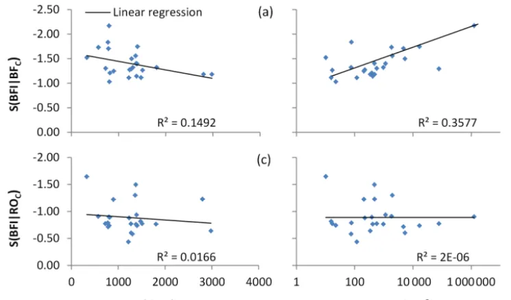
Figure 1.Scatterplots of sensitivity indices vs. time series (n) and drainage area of the 24 US basins. The watershed area uses a logarithmic axis, while the others are linear axes.
to year changes in the elevation of the water table may result in temporal changes in BFC. They recommended taking dif-ferent BFCvalues per year based on the conductivity values during low-flow periods to avoid the effects of temporal fluc-tuations in BFC.
The sensitivity index of BFI for BFCshows a decreasing trend with the increase in time series (n) (Fig. 1a) and an in-creasing trend with inin-creasing watershed area (Fig. 1b), with correlation coefficients of 0.1492 and 0.3577, respectively. Although the correlations are not obvious, they have impor-tant guiding significance. Large basins comprise many dif-ferent subsurface flow paths contributing to streams (Okello et al., 2018), each of which has a unique conductivity value (Miller et al., 2014). Furthermore, it is difficult to represent the conductivity characteristics of subsurface flow with a spe-cial value. Therefore, the CMB method has higher applicabil-ity to long time series for small watersheds.
The sensitivity index of BFI for ROCdid not change sig-nificantly with the increase in time series and watershed area (Fig. 1c and d). During rainstorms, the conductivity of streams became similar to that of the rainfall (Stewart et al., 2007). The electrical conductivity of rainfall varies slightly by region, is usually at a fixed value, and has no significant relationship with the basin area and year (Munyaneza et al., 2012). Therefore, the temporal and spatial variation charac-teristics of BFI for ROCare not obvious.
Genereux’s method (Eq. 19) estimates the average un-certainty in BFI in the 24 basins (average of mean Wfbf) to be 0.20, whereas the average uncertainty in BFI (aver-age ofWBFI) calculated directly using the proposed method (Eq. 23) is 0.11 (Table 1). Mean Wfbf in each basin is generally larger than WBFI (WBFI is about 0.51 times of
Figure 2.Scatterplot of uncertainty in BFI (WBFI) and mean
uncer-tainty infbf(meanWfbf).
mean Wfbf), and there is a significant linear correlation (Fig. 2). This shows that the two methods have the same volatility characteristics for BFI uncertainty estimation, but Genereux’s method (Eq. 19) often overestimates the uncer-tainty in BFI. This also means that when the time series is longer than 365 days, the measurement errors in conductiv-ity and streamflow will cancel each other out and thus reduce the uncertainty in BFI (about half of the original).
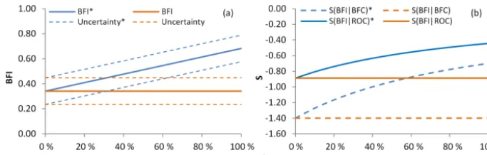
[image:6.612.325.530.339.475.2]Figure 3.Estimation results of(a)baseflow index and uncertainty(b)sensitivity indices, under different low-conductivity soil flow ratios, assuming high-conductivity baseflow remains unchanged. An asterisk indicates the results of the estimation considering the low-conductivity soil flow.
CMB method comprised only the baseflow index of the deep subsurface flow. The parameter sensitivity indices and uncer-tainty in the deep subsurface flow were also calculated by the methods of this paper. Cartwright et al. (2014) showed that the ratio of low-conductivity soil flow to high-conductivity subsurface flow in the Barwon Basin in southeastern Aus-tralia is close to 1. If only the BFI doubles and other parame-ters remain unchanged, then the sensitivity indices calculated by Eqs. (9) and (10) are halved, whereas the uncertainty cal-culated by Eq. (23) remains unchanged. Therefore, noncon-stant soil flow conductivity may lead to an overestimation of sensitivity, but it has less impact on uncertainty estimates.
To better understand the effects of low-conductivity soil flow on BFI, parameter sensitivity, and the uncertainty esti-mation results, this study assumed that the high-conductivity baseflow is constant and the ratio of low-conductivity soil flow to high-conductivity baseflow (SF/BF) is between 0 and 1. Based on the average values of the 24 watersheds mentioned in Table 1, the estimation results with and with-out consideration of low-conductivity soil flow were ana-lyzed (Fig. 3). The CMB method used in this study neglects low-conductivity soil flow; thus, the BFI, sensitivity indices, and uncertainty do not change with a change in SF/BF (or-ange line in Fig. 3). When the low-conductivity soil flow is considered in the estimations, the BFI value is found to in-crease linearly with the inin-crease in SF/BF (blue solid line in Fig. 3a); the absolute values of sensitivity indices decrease nonlinearly with the increase in SF/BF; and the difference between S(BFI|BFc)and S(BFI|ROc) decreases gradually (blue line in Fig. 3b). The uncertainty in BFI does not fluctu-ate with changes in SF/BF (blue dashed line in Fig. 3a). In general, the deviation between BFI, sensitivity indices, and the “true values” gradually increases with an increase in the low-conductivity soil flow of a basin.
5 Conclusions
This study analyzed the sensitivity of BFI, calculated using the CMB method, to errors or uncertainties in the parame-ters BFCand ROCand the variablesyk and SCk. In addition,
the uncertainty in BFI was calculated. The equations derived in this study (Eqs. 9 and 10) could calculate the sensitivity indices of BFI for BFCand ROC. For time series longer than 365 days, the measurement errors in conductivity and stream-flow exhibited a mutual offset effect, and their influence on BFI could be neglected. Considering the mutual offset, the uncertainty in BFI would be halved. From this perspective, Eq. (23) could estimate the uncertainty in BFI for time se-ries longer than 365 days. The application of the method to 24 basins in the US showed that BFI is more sensitive to BFC. Future studies should dedicate more effort to determining the value of BFC. In addition, the CMB method may be more suitable for long time series of small watersheds.
Systematic errors in specific conductance and streamflow as well as temporal and spatial variations in baseflow con-ductivity may be the main sources of BFI uncertainty. Better rating curves are probably more important than better log-gers, and understanding the specific conductance of baseflow is likely more important than understanding that of surface runoff.
The above conclusions were drawn only from the average of the studied 24 basins, and further research in other coun-tries or in more watersheds is thus required. This study fo-cused on the two-component hydrograph separation method with conductivity as a tracer, but parameter sensitivity analy-sis and uncertainty analyanaly-sis methods involving other tracers are similar. Therefore, similar equations can easily be derived by referring to the findings of this study.
Appendix A: Calculation of the partial derivatives
∂bk ∂BFc
= ∂
∂BFc
yk(SCk−ROc) BFc−ROc
=yk(SCk−ROc)
∂ ∂BFc
1
BFc−ROc= −yk
SCk−ROc
(BFc−ROc)2
, (A1)
∂bk ∂ROc
= ∂
∂ROc
yk(SCk−ROc) BFc−ROc
=yk ∂ ∂ROc
SCk−ROc BFc−ROc
=yk
−(BFc−ROc)+(SCk−ROc) (BFc−ROc)2
=yk SCk−BFc
(BFc−ROc)2, (A2)
∂BFI
∂BFc =
∂ ∂BFc b y = 1 y n X k=1 ∂bk ∂BFc =1 y n X k=1
−yk
SCk−ROc (BFc−ROc)2
(see Eq.A1)
= 1
y(BFc−ROc)2
n X
k=1
(ykROc−ykSCk)
=
yROc−
n P
k=1
ykSCk y(BFc−ROc)2
, (A3)
∂BFI
∂ROc
= ∂
∂ROc
b y = 1 y n X k=1 ∂bk ∂ROc
= 1 y n X k=1 yk
SCk−BFc
(BFc−ROc)2
(see Eq.A2)
= 1
y(BFc−ROc)2
n X
k=1
(ykSCk−ykBFc)
=
n P
k=1
ykSCk−yBFc
y(BFc−ROc)2
, (A4)
∂bk ∂SCk
= ∂
∂Qck
yk(SCk−ROc) BFc−ROc =
1 BFc−ROc
∂ ∂SCk yk(SCk−ROc)=
yk
BFc−ROc
, (A5)
∂bk ∂yk
= ∂
∂yk
yk(SCk−ROc) BFc−ROc
=(SCk−ROc)
BFc−ROc
∂ ∂yk
yk
=SCk−ROc
BFc−ROc
, (A6)
∂BFI
∂SCk
= ∂
∂SCk b y = 1 y n X k=1 ∂bk ∂SCk
=1 y n X k=1 yk
BFc−ROc
(see Eq.A5)= 1
y (BFc−ROc)
n X
k=1
yk
= 1
BFc−ROc, (A7)
∂BFI ∂yk = ∂ ∂yk b y = ∂ ∂yk n P k=1 bk n P k=1 yk = n P k=1 bk 0 n P k=1 yk − n P k=1 bk n P k=1 yk 0 n P k=1 yk 2 = y n P k=1 bk
0−b
n P k=1 yk 0 y2 = y n P k=1
SCk−ROc
BFc−ROc
−nb
y2 (see Eq.A6)
=
y n P
k=1
(SCk−ROc)−nb (BFc−ROc)
y2(BF
c−ROc)
=
n P
k=1
(SCk−ROc)−nBFI(BFc−ROc)
y (BFc−ROc) . (A8)
Appendix B: Calculation of the sensitivity indices
S (BFI|BFc)=
1BFcBFI
BFI
1BFc
BFc
=
yROc−
n P k=1
ykSCk y(BFc−ROc)2
1BFc BFc BFI1BFc
(see Eq.7)=
BFc
yROc−
n P k=1
ykSCk
S (BFI|ROc)=1ROcBFI
BFI
1RO
c ROc
=
n P
k=1
ykSCk−yBFc
y(BFc−ROc)2
1ROc ROc BFI1ROc
(see Eq.8)=
ROc
n
P
k=1
ykSCk−yBFc
yBFI(BFc−ROc) 2
. (B2)
Appendix C: Proof that∂BFI/∂ykis far less than 1 day m−3
∂BFI
∂yk = n P k=1
(SCk−ROc)−nBFI(BFc−ROc)
y (BFc−ROc)
(see Eq.A8). (C1)
Because ofn >0, BFI>0 (BFC−ROC) >0, the above for-mula can be simplified:
∂BFI
∂yk <
n P k=1
(SCk−ROc)
y (BFc−ROc)
. (C2)
Since BFC is usually much larger than SCk, the above
for-mula can be rewritten as
∂BFI
∂yk
<
n
P
k=1
(BFc−ROc)
y (BFc−ROc)
=n (BFc−ROc)
y (BFc−ROc)
= n
y =
1
y. (C3)
Supplement. The supplement related to this article is available online at: https://doi.org/10.5194/hess-23-1103-2019-supplement.
Author contributions. WY, CX, and XL developed the research train of thought. WY and CX completed the parameters’ sensitivity analysis. XL completed the uncertainty estimate of BFI. WY car-ried out most of the data analysis and prepared the manuscript with contributions from all coauthors.
Competing interests. The authors declare that they have no conflict of interest.
Acknowledgements. This work is supported by the National Natural Science Foundation of China (41572216), the Provincial School Co-construction Project Special – Leading Technology Guide (SXGJQY2017-6), the China Geological Survey Shenyang Geological Survey Center “Changji Economic Circle Geological Environment Survey” project (121201007000150012), and the Jilin Province Key Geological Foundation Project (2014-13). We thank the anonymous reviewers for useful comments to improve the manuscript.
Edited by: Markus Hrachowitz Reviewed by: three anonymous referees
References
Cartwright, I., Gilfedder, B., and Hofmann, H.: Contrasts between estimates of baseflow help discern multiple sources of wa-ter contributing to rivers, Hydrol. Earth Syst. Sci., 18, 15–30, https://doi.org/10.5194/hess-18-15-2014, 2014.
Costelloe, J. F., Peterson, T. J., Halbert, K., Western, A. W., and McDonnell, J. J.: Groundwater surface mapping informs sources of catchment baseflow, Hydrol. Earth Syst. Sci., 19, 1599–1613, https://doi.org/10.5194/hess-19-1599-2015, 2015.
Eckhardt, K.: How to construct recursive digital filters for baseflow separation, Hydrol. Process., 19, 507–515, https://doi.org/10.1002/hyp.5675, 2005.
Eckhardt, K.: Technical Note: Analytical sensitivity analysis of a two parameter recursive digital baseflow separation filter, Hy-drol. Earth Syst. Sci., 16, 451–455, https://doi.org/10.5194/hess-16-451-2012, 2012.
Ernest, L.: Gaussian error propagation applied to ecological data: Post-ice-storm-downed woody biomass, Ecol. Monogr., 75, 451– 466, https://doi.org/10.1890/05-0030, 2005.
Genereux, D.: Quantifying uncertainty in tracer-based hy-drograph separations, Water Resour. Res., 34, 915–919, https://doi.org/10.1029/98wr00010, 1998.
Hamilton, A. S. and Moore, R. D.: Quantifying Uncertainty in Streamflow Records, Can. Water Resour. J., 37, 3–21, https://doi.org/10.4296/cwrj3701865, 2012.
Huang, Z. P. and Chen, Y. F.: Hydrological statistics, China Wa-ter & Power Press, Beijing, China, 2011.
Kline, S. J.: The purposes of uncertainty analysis, J. Fluids Eng., 107, 153–160, 1985.
Lott, D. A. and Stewart, M. T.: Base flow separation: A comparison of analytical and mass balance methods, J. Hydrol., 535, 525– 533, https://doi.org/10.1016/j.jhydrol.2016.01.063, 2016. Mei, Y. and Anagnostou, E. N.: A hydrograph separation method
based on information from rainfall and runoff records, J. Hydrol., 523, 636–649, https://doi.org/10.1016/j.jhydrol.2015.01.083, 2015.
Miller, M. P., Susong, D. D., Shope, C. L., Heilweil, V. M., and Stolp, B. J.: Continuous estimation of baseflow in snowmelt-dominated streams and rivers in the Upper Colorado River Basin: A chemical hydrograph separation approach, Water Resour. Res., 50, 6986–6999, https://doi.org/10.1002/2013WR014939, 2014. Munyaneza, O., Wenninger, J., and Uhlenbrook, S.: Identification of
runoff generation processes using hydrometric and tracer meth-ods in a meso-scale catchment in Rwanda, Hydrol. Earth Syst. Sci., 16, 1991–2004, https://doi.org/10.5194/hess-16-1991-2012, 2012.
NWIS: US Geological Survey’s National Water Information Sys-tem, available at: http://waterdata.usgs.gov/nwis, last access: September 2018.
Okello, A. M. L. S., Uhlenbrook, S., Jewitt, G. P. W., Masih, L., Riddell, E. S., and Zaag, P.V.: Hydrograph separation us-ing tracers and digital filters to quantify runoff components in a semi-arid mesoscale catchment, Hydrol. Process., 32, 1334– 1350, https://doi.org/10.1002/hyp.11491, 2018.
Stewart, M., Cimino, J., and Rorr, M.: Calibration of base flow sepa-ration methods with streamflow conductivity, Ground Water, 45, 17–27, https://doi.org/10.1111/j.1745-6584.2006.00263.x, 2007. Taylor, J. R.: An Introduction to Error Analysis: The Study of Un-certainties in Physical Measurements, Univ. Sci. Books, Mill Val-ley, Calif., 1982.
Wagner, R. J., Boulger Jr., R. W., Oblinger, C. J., and Smith, B. A.: Guidelines and standard procedures for continuous water-quality monitors-Station operation, record computation, and data report-ing, US Geol. Surv. Tech. Meth. 1-D3, US Geological Survey, Reston, Virginia, 51 pp., 2006.