Munich Personal RePEc Archive
Fine-tuning the equivalent strike
framework for bespoke cdo tranches
pricing
Mrad, Moez and Triki, Racem
30 March 2011
Online at
https://mpra.ub.uni-muenchen.de/30750/
Fine-tuning the Equivalent Strike framework
for Bespoke CDO Pricing
Moez MRAD
∗Racem TRIKI
†30 March 2011
Abstract
1
This paper presents a fine-tuning of some mapping functions used in the Equivalent Strike framework. This new approach provides an equivalent strike that is independent from the index base correlation. This feature is valuable when pricing very junior and senior tranches or when computing index tranches (or index base correlation) sensitiv-ities. Our numerical tests on realistic cases showed that the equivalent correlation provided by this new is pretty close to what is computed with common mapping functions.
Key words: Bespoke CDO pricing, Equivalent Strike framework, Index base correlation extrapolation, Index tranche sensitivities.
JEL classification: C00, C61, C62
1
Introduction
Equivalent strike techniques are widely used in order to price and hedge synthetic bespoke CDO tranches in the base correlation framework. In this framework the attachment and detachment correlations of a bespoke tranche are deduced from base correlations of liquid index tranches via mapping techniques. There are several mapping techniques - of which the advantages and drawbacks have been widely discussed in the literature (see [1], [2], [3])
-∗Cr´edit Agricole Corporate and Investment Bank - [email protected] †Cr´edit Agricole Corporate and Investment Bank - [email protected]
1
such as: At The Money or Probability Matching or Expected Tranche Loss. When looking for an equivalent strike - at a given maturity - the common approach consists in solving the following optimization problem:
min
K φ(K, ρI(K)) (1)
where φ is a bivariate function depending on the unknown K and the base correlation curve of the index to which we are mapping ρI : K 7→ ρI(K)
(to simplify notations, we omit the dependence on maturity throughout the paper). The equivalent strike solution of Problem (1):
K⋆ = argmin
Kφ(K, ρI(K)) (2)
clearly depends on the shape of the base correlation curve ρI. This behavior
should be taken into account when dealing with the situations below:
1. Pricing very junior or senior tranches: Since mid-2007, traders are more likely to price very junior tranches detaching below 3% (due to the subordination erosion of some junior tranches present in their book by successive default events) or very senior tranches attaching above 30% in order to hedge the book and take into account new market conditions (it is common now to see quotes for [60%,100%] tranches). For these particular tranches, the equivalent strike K⋆ may depend on
the extrapolation hypothesis of the base correlation curve ρI.
2. Hedging a bespoke product via liquid index tranches: Since the Equiva-lent Strike approach consists in mapping a bespoke tranche to a liquid index tranche market, it is important to compute the sensitivity of the bespoke tranche to the tranches of the liquid index. This is achieved by perturbing the market quotes of each index tranche, bootstrapping the base correlation for each perturbation scenario and finally valuing the bespoke tranche via the Equivalent Strike approach for each index correlation scenario. Since the equivalent strike K⋆ depends on the
index correlation curve ρI, it has to be computed for each index base
correlation scenario. The index tranche sensitivity computation time will be impacted by this step.
property of the proposed method is that the equivalent strike is indepen-dent from the index base correlation ρI while the equivalent base correlation ρI(K⋆) is close to what is provided by the common approach described by
Equation (1). The second section of this paper provides a brief overview of major mapping techniques within the Equivalent Strike framework. The third section is dedicated to the description of the new mapping criterion. The final section gives numerical results and compares our approach to the common approach described by Equation (1).
2
Review of common mapping methods
Although some well-known drawbacks, the base correlation approach is widely used by practitioners in order to price CDO tranches. In this framework a protection leg [K1, K2] can be valued as the [0, K2]-protection leg value (using
a correlation ρ2) minus the [0, K1]-protection leg value (using a correlationρ1
that may be different fromρ2). When [K1, K2] is a bespoke CDO tranche the
attachment and detachment correlations ρ1 and ρ2 are deduced from liquid
index correlation market data via a mapping technique. For a given bespoke equity tranche [0, KB] the mapping technique provides an equivalent index
equity tranche [0, K⋆
I]. The correlation used to price the [0, KB]-tranche is
then provided by ρ⋆
B =ρI(KI⋆) (where ρI : K 7→ ρI(K) is the base
correla-tion curve of the index used for mapping). In practice, the problem means finding the strike K⋆
I that verifies:
ψ(K⋆
I, ρI(KI⋆), πI) =ψ(KB, ρI(KI⋆), πB) (3)
where:
• ψ is the mapping function (it needs to be monotonic of the strike)
• πI (resp. πB) is the index (resp. bespoke) portfolio
• KB is the given bespoke equity tranche strike
• K⋆
I the strike that allow to verify Equation (3)
2.1
At The Money (ATM)
This is one of the first and simplest mapping functions that have been used in the Equivalent strike framework. It is defined by:
ψ(K, ρ, π) = K
E[L(π)]
where E is the expectation operator and L(π) is the loss of the portfolio
π. This choice of mapping function leads to a simple expression for the equivalent strike (that is not dependant on the shape of the base correlation
ρI):
K⋆
I =KB×
E[L(
πI)] E[L(πB)]
If the bespoke portfolio is tighter than the index portfolio, the bespoke equity tranche will be mapped to a more senior index tranche and conversely. This may lead to a situation (especially in the stochastic recovery framework) where the Equivalent strikeK⋆
I is higher than 100%. Other drawbacks of this
mapping function are the independence from the portfolios dispersions and non continuity with respect to default settlement. In term of advantages one can mention that the equivalent strike computation is extremely fast (by comparison to other mapping functions) and that K⋆
I is independent
fromρI which is an appreciable feature when dealing with the two situations
mentioned in the introduction.
2.2
Probability Matching (PM)
In this case the mapping function is the probability that the loss of the portfolio π is below the strike K. The equivalent strike:
ψ(K, ρ, π) = Pρ[L(π)≤K]
where Pρ is the probability operator using correlation value ρ and L(π) is
the loss of the portfolio π.
This mapping function addresses some of the drawbacks of the ATM map-ping since it is sensitive to portfolios dispersion and is continuous with respect the to default settlement. Under normal market conditions ψ(0, ρ, π) > 0. Thus, when using this mapping function one can face situations (typically when index portfolio is much tighter than the bespoke one), where there is no strike K⋆
I such as Equation (3) is verified. This mapping function may also
has a higher WAS (weighted average spread) than the index portfolio, the intuition is that the equivalent strike of the reference will be lower than the bespoke strike (similar to the ATM case), but this may not be the case as the equivalent strike depends on the dispersion of the portfolio and the index cor-relation curve level. In a Constant Recovery framework, solving Equation (3) may be numerically unstable (since the portfolio loss cumulative distribution is discrete for a given correlation). Smoothing the cumulative distribution functions allows overcoming this behavior.
2.3
Expected Tranche Loss (ETL)
The mapping function is the proportion of the expected portfolio loss that is embodied in a given equity tranche. It is a monotonic function of the strike:
ψ(K, ρ, π) = Eρ[min (L(π), K)]
E[L(π)]
where Eρ is the expectation operator using correlation value ρ and L(π) is
the loss of the portfolio π.
This mapping function takes into account the dispersion of portfolios (similar to the Probability Matching case). It always provides an equivalent strike since: (i) we are dealing with a mapping function that is monotonic of the strike and (ii) we have ψ(0, ρ, π) = 0 and ψ(1, ρ, π) = 1 (we assume here that we are dealing with standard portfolios. i.e. containing no short names). This mapping function has also the following drawbacks: (1) Sometimes it take dispersions into account but in a counterintuitive way. This is the case for example, when an issuer of the bespoke portfolio widens idiosyncratically. (2) Another problem is the continuity with respect to default settlement.
This method like the Probability Matching, leads to an equivalent strike that is dependent on the index base correlation curve ρI. Particularly, when
mapping a junior bespoke tranche to an index portfolio that is much wider than the bespoke one, the equivalent strike is sensitive the extrapolation hypothesis below the lowest market strike (typically 3%). The same thing may also happen, when we map a super-senior tranche on a bespoke portfolio that is extremely tighter than the index one. This time the equivalent strike is sensitive to the extrapolation hypothesis above the biggest market strike.
3
New computation method
of the following problem:
K⋆ = argmin
Kϕ(K)
where the function ϕ is defined via the mapping function ψ by:
ϕ(K) =[
ψ(K, ρI(K), πI)−ψ(KB, ρI(K), πB)
]2
(4)
This mean that the equivalent strike is a function of the index correlation curve ρI : K 7→ ρI (K). We suppose that ρI ∈ C
1
[0,1], where C1
[0,1] is the set of continuously differentiable functions from [0,1] to R. This set is a Banach Space with respect to the C1
-norm defined by:
∥f ∥C1=∥f ∥∞+∥f ′
∥∞, ∀f ∈ C
1
[0,1]
where ∥ • ∥∞ stands for the sup-norm. We also introduce the function
F :C1
[0,1]→Rsuch that:
K⋆ =F (ρ I)
We assume that F is Gateaux differentiable at ρI and we denote dFρI its
Gateaux derivative at this point. The bespoke equity tranche is valued using the equivalent correlation:
ρ⋆ =ρ
I(F(ρI)), ρ⋆ ∈[0,1]
Let h : K 7→ h(K) be a vector in the Banach space C1
[0,1]. We look at the first order impact of a small perturbation in the direction of h on the equivalent correlation ρ⋆. Let ε be a real number such as: 0 ≤ ε ≪ 1. We
denoteρ⋆
ε = (ρI+εh)(F(ρI+εh)) and we expand this expression to the first
order:
ρ⋆ ε =ρ
⋆ +ε(ρ′
I(K ⋆)dF
ρI(h) +h(K
⋆)) +o(ε) (5)
The term ερ′
I(K⋆)dFρI(h) is due to the fact that in the common Equivalent
Strike framework, K⋆ depends on the index correlation curve ρ
I. This term
disappears when the mapping function is not dependent on the correlation curve ρI like in ATM approach. The second term εh(K⋆) is not peculiar
to the Equivalent Strike framework and will always exist. We propose in this section, to change the Equivalent strike computation method, in order to remove the dependance on the index correlation curve ρI while keeping
sensitivity to the bespoke and index portfolios dispersions. We will see in the next section that this new approach provides similar results to the common market practice. We propose instead of minimizing the functionϕintroduced in Equation (4) to minimize the function χdefined by:
χ(K) =
∫ 1 [
ψ(K, ρ, πI)−ψ(K
B, ρ, πB)
]2
The new equivalent strike is then computed as the solution of the following problem:
ˆ
K = argminKχ(K)
and the correlation used to price the equity bespoke tranche is ˆρ = ρI( ˆK).
If we look as earlier at the first order impact of a small perturbation in the direction h whereh∈ C1
[0,1] on the correlation ˆρ, the perturbed correlation ˆ
ρε (where the real ε verifies 0≤ε≪1) is given by:
ˆ
ρε = ˆρ+εh(K⋆) +o(ε) (7)
In practice, we will use the following objective function:
χD(K) =
1 N N ∑ i=1 [
ψ(K, ρi, πI)−ψ(KB, ρi, πB)
]2
(8)
where N is the number of correlation levels. The quantities ψ(KB, ρi, πB), i ∈< 1, N > are totally known and they can be pre-computed and stored when looking for ˆK. This will reduce computation time. If we apply this approach to the Probability Matching method the objective function defined by Equation (8) becomes:
χD(K) =
1 N N ∑ i=1 [ Pρi
[
L(
πI)
≤K]
−Pρi [
L(
πB)
≤KB
]]2
(9)
Whereas when we apply this approach to the Expected Tranche Loss Match-ing method the objective function defined by Equation (8) becomes:
χD(K) =
1 N N ∑ i=1 [ Eρi
[
min(
L(
πI)
, K)] E[L(πI)] −
Eρi [
min(
L(
πB)
, KB
)]
E[L(πB)]
]2
(10) In the next section, we will study the behavior of this new approach with respect to the number of correlation levels N, the portfolios WAS (Weighted Average Spread)... . The results will be compared to those obtained in the common Equivalent Strike framework.
4
Numerical tests:
In this section, we mainly focus on the ETL mapping (since it is more used by practitioners than Probability Matching or any other mapping function). We define the ratio:
where the WAS is given by:
WAS =
M
∑
m=1
wmDmSm/ M
∑
m=1
wmDm
with: M the number of issuers and Dm, Sm, wm are respectively the risky
duration, the market spread and the weight of the issuer m, m= 1, ..., M in the portfolio.
4.1
Impact of the ratio
ω
We use the mapping function (10) with 10 correlation levels ρi = i/9; i =
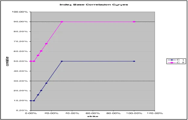
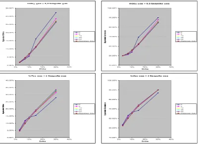
0, ...,9 and we compare both approaches for ω ∈ {0.25,0.5,2,4}. We also consider 2 different index base correlation curves C1 (low correlation
[image:9.595.141.454.360.560.2]envi-ronment) and C2 (high correlation environment):
Figure 1: 5-years index base correlation
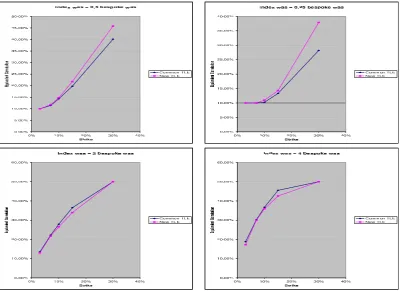
Figure 2: Common TLE and New TLE with low index base correlation
We notice that when index portfolio’s WAS is smaller (respectively bigger) than bespoke portfolio’s WAS, the equivalent base correlation provided by Common TLE is below (respectively above) the one provided by New TLE. The difference between both methods is bigger when ω = 0.25 or 4 than when ω = 0.5 or 2. We also notice that new and Common TLE are closer for junior tranches (see graphs for ω= 2 or 4).
We now look at the the behavior of Common TLE and New TLE as a function of the ratio ω in high correlation environment (i.e. using the curve
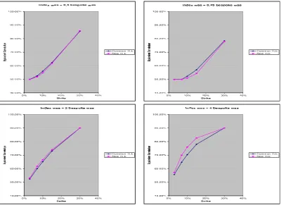
Figure 3: Common TLE and New TLE with high index base correlation
In high correlation environment, the equivalent base correlation curves relative positions is the opposite of what is observed the low correlation environment. When index portfolio’s WAS is smaller (respectively bigger) than bespoke portfolio’s WAS the equivalent base correlation provided by Common TLE is above (respectively below) the one provided by New TLE. Here too, the difference between both methods is bigger when ω= 0.25 or 4 than when ω = 0.5 or 2. We also notice that for ω = 0.5 or 2 base correla-tion curves are close in high correlacorrela-tion environment that in low correlacorrela-tion environment.
4.2
Impact of the number of correlation levels
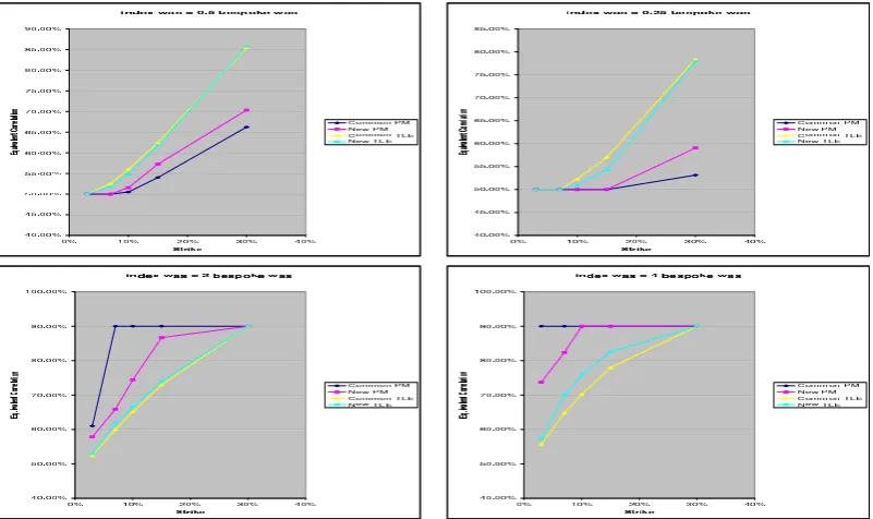
We use the mapping function (10) with a number of correlation levels N ∈ {2,5,10,20,50} and we compare both approaches for ω ∈ {0.5,2}. We also consider as in the previous paragraph the curves C1 and C2.
when using the curve C1:
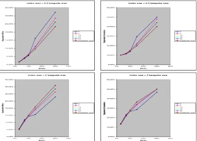
Figure 4: Impact of correlation levels number on New TLE with low index base correlation
We notice a convergence of the equivalent strike from N = 10. Except for N = 2, we observe that the equivalent strike obtained by New TLE decreases as the N increases when the index portfolio is tighter than the bespoke one. The equivalent strike obtained with Common TLE is higher than those obtained by New TLE. Conversely, when the index portfolio is wider than the bespoke one the equivalent strike decreases as N increases (Except for N = 2). The equivalent strike obtained with Common TLE is lower than those obtained by New TLE.
Figure 5: Impact of correlation levels number on New TLE with high index base correlation
By construction, New TLE gives the same equivalent strikes as with C1.
We notice that the equivalent strikes obtained via Common TLE are closer to the one obtained with New TLE.
4.3
Comparison of PM and ETL mapping
In this paragraph, we compare the results obtained by the common and new approaches for PM and ETL mappings using the same conditions as in paragraph 4.1. We provide below the equivalent correlations for the curves
Figure 6: PM and TLE with low index base correlation
[image:14.595.110.511.434.672.2]We notice that with either common or new approach, TLE mapping is smoother than PM mapping (PM gives an equivalent correlation of which the shape is as discontinuous as the index base correlation). We also notice that TLE provides lower (resp. higher) equivalent base correlations then PM when the ration ω > 1 (resp. ω < 1). We also observe that Common and New TLE equivalent base correlation are more close than Common and New PM ones. More generally, we notice that the equivalent base correlation shape and behavior mainly depends on the mapping function (PM vs ETL) rather than the fine-tuning approach (Common vs New).
4.4
Stability of Common and New ETL mapping
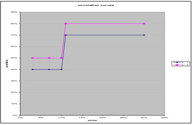
[image:15.595.141.454.357.560.2]In this section we look at the equivalent base correlation sensitivity behavior. Thus, we consider the following extreme example of 2 discontinuous index base correlation curves C1 and C2:
Figure 8: 5-years index base correlation
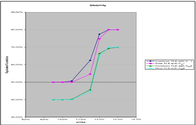
Figure 9: Stability of the equivalent correlation sensitivity w.r.t. strike
When using New TLE, we notice that a bump in the index base corre-lation of 10% leads to a bump in the equivalent strike of a 10% as expected from Equation (7). When using Common TLE, we notice that the equivalent correlation variation is 16.8% which is much higher (The extra bump of 6.8% is associated to the term ερ′
I(K⋆)dFρI(h) appearing in Equation (5)).
Be-sides, we notice a ”discontinuity” of the equivalent base correlation variation around the strike 10.5% (with Common TLE, the equivalent base correlation variation is close to 10% at strikes 10% and 11%).
4.5
Impact of extrapolation on ETL mapping
In this paragraph, we look at the impact of the extrapolation method for ETL mapping. We consider a bespoke and index portfolios such us ω = 2 and we focus on the left side extrapolation. We consider the curve C2 introduced in
paragraph 4.1 with 3 extrapolations:
E1 Flat extrapolation after the strike 30%
E2 Linear extrapolation after the strike 30% with a slope equal to the slope
between 15% and 30%
E3 Linear extrapolation after the strike 30% with a slope twice bigger than
We then look at the equivalent strike and correlations associated with a bespoke strike of 30% for the 3 extrapolations introduced above:
Equivalent strike as a function of the left extrapolation slope:
slope 0 1 2
Common TLE 32.51% 32.22% 31.98% New TLE 32.53% 32.53% 32.53%
Equivalent correlation as a function of the left extrapolation slope:
slope 0 1 2
Common TLE 90% 92.22% 93.97%
ρI(32.51%) 90% 92.51% 95.01%
New TLE 90% 93.53% 95.05%
The difference between the equivalent correlation provided by Common TLE and ρI(32.51%) is mainly due to the dependance of the Common TLE
on the index curve ρI. This leads to the following break-even for the
[30%,100%] super-senior tranche:
Break-even spread as a function of the left extrapolation slope:
slope 0 1 2
Common TLE 0.62% 0.67% 0.72%
ρI(32.51%) 0.62% 0.68% 0.75%
New TLE 0.62% 0.68% 0.75%
We see that extrapolation E3 impact in Common TLE is about 3 bps.
4.6
Real case
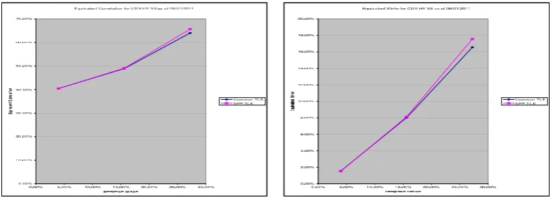
Figure 10: CDX HY S9 mapped via Common and New TLE to CDX IG S9
We notice that both methods give very close results. We did many tests with other portfolios. They all showed that Common and New TLE results are close.
4.7
Index tranche sensitivities
We consider a 100 Mio USD, 5-years [3.981%,15.609%]-tranche on CDX HY S9. We first, price this tranche (regarded as bespoke) as of 06/01/2011 with Common and New TLE using CDX IG S9 as a reference index. We provide in the following table the prices given by both TLE approaches 2
:
TLE Price in USD Eq. att. strike Eq. att. correl. Eq. det. strike Eq. det. correl Common 44,034,611 1.348% 43.887% 7.071% 50.524%
New 44,036,069 1.290% 43.887% 7.070% 50.521%
Table 1: Pricing outputs
We then, provide the hedge in Mio of USD of this bespoke tranche with junior 5Y tranches of CDX IG S9
2
TLE [0- 2.36] [2.36 - 6.49] [6.49 - 9.59] [9.59 - 14.76] [14.76 - 30.25] Total Common 24,572,935 92,400,206 12,522,328 0 0 129,495,469
[image:19.595.101.543.129.172.2]New 22,092,188 88,177,749 11,926,527 0 0 122,196,464
Table 2: Tranche notional of hedging CDX IG S9 5Y tranches
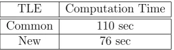
Both approaches provide similar hedging figures (even if the hedge with New TLE is slightly below the one provided by Common TLE). The advan-tage of New TLE approach is that it is faster than Common TLE approach. Actually, when computing the hedges above, one has to compute the equiva-lent correlations (and thus strikes) for different perturbation scenarios of the CDX IG S9 tranches market up-front quotes (and thus for different pertur-bation scenarios of the 5Y-CDX IG S9 base correlation curve). In the New TLE approach the equivalent strike are computed only once (when comput-ing the price) which reduces the computation time. We provide below the computation time for these 2 approaches using a computation grid3
:
TLE Computation Time Common 110 sec
New 76 sec
Table 3: Index tranche hedging batch computation time
5
Conclusion
We presented a fine-tuning of some mapping functions used in the Equivalent Strike framework. In this approach, the equivalent strike is independent from the index base correlation shape. Our numerical tests showed that the new approach is more stable than the common one. For realistic cases, the equivalent correlations obtained via New or Common TLE approaches are very close.
Fine-tuned mapping functions behave similarly to the common ones as functions of portfolios dispersions and ratio of portfolio WAS. Nevertheless, they have the advantage of providing an equivalent strike independent from the index base correlation shape. In particular, equivalent strikes are not sensitive to extrapolation (and even interpolation) hypothesis. This feature
3
[image:19.595.213.384.386.435.2]makes the index tranche hedging computation of a bespoke tranche with the new approach faster than what it can be achieved with the common approach.
References
[1] Quantitative Research (2007-Q1). Base Correlation Mapping. Lehman Brothers.
[2] Prasun Baheti, Sam Morgan, (2007-Q2/Q3). Impact of Spread Disper-sion and Correlation Level on TLP Mapping. Lehman Brothers.