Damping of a Simple Pendulum Due to Drag on Its String

(1)

http://www.scirp.org/journal/jamp ISSN Online: 2327-4379

ISSN Print: 2327-4352

Damping of a Simple Pendulum Due to

Drag on Its String

Pirooz Mohazzabi, Siva P. Shankar

Department of Mathematics and Physics, University of Wisconsin-Parkside, Kenosha, WI, USA

Abstract

A basic classical example of simple harmonic motion is the simple pendulum, consisting of a small bob and a massless string. In a vacuum with zero air re-sistance, such a pendulum will continue to oscillate indefinitely with a con-stant amplitude. However, the amplitude of a simple pendulum oscillating in air continuously decreases as its mechanical energy is gradually lost due to air resistance. To this end, it is generally perceived that the main role in the dis-sipation of mechanical energy is played by the bob of the pendulum, and that the string’s contribution is negligible. The purpose of this research is to expe-rimentally investigate the merit of this assumption. Thus, we expeexpe-rimentally investigate the damping of a simple pendulum as a function of its string di-ameter and compare that to the contribution from its bob. We find out that although in some cases the effect of the string might be small or even negligi-ble, in general the string can play a significant role, and in some cases even a greater role on the damping of the pendulum than its bob.

Keywords

Simple Pendulum, String, Damping, Air Resistance, Drag

1. Introduction

Perhaps the simplest oscillating system is a small object attached to a string of negligible mass, known as simple pendulum. If the amplitude of oscillations is small, the pendulum oscillates with a period T which is independent of the am-plitude and is given by

2π L T

g

= (1)

where L is the length of the pendulum and g is the acceleration due to gravity (9.80 m/s2_{). In the absence of frictional losses, the hypothetical pendulum would} How to cite this paper: Mohazzabi, P. and

Shankar, S.P. (2017) Damping of a Simple Pendulum Due to Drag on Its String. Jour-nal of Applied Mathematics and Physics, 5, 122-130.

http://dx.doi.org/10.4236/jamp.2017.51013

Received: December 27, 2016 Accepted: January 22, 2017 Published: January 25, 2017

(2)

oscillate indefinitely. However, the amplitude of oscillations of any real undriven mechanical pendulum, including simple pendulum, continuously decreases as a result of frictional losses, mainly due to air resistance while its period and fre-quency remain constant. To this end, the general assumption is that the drag force due to the air resistance on the bob of the pendulum is the cause of its damping, and normally the air resistance on the string of the pendulum is as-sumed to be negligibly small.

In order to be able to measure the gravitational acceleration very accurately, Nelson and Olsson [1] theoretically investigated the effect of air resistance on the bob as well as the string of a simple pendulum. However, they did not dis-cuss the relative importance of these effects. Later on, Dunn [2] experimentally studied the damping effect of the string on a pendulum by varying the length of the string and the diameter of the bob, but did not mention what the diameter of the string was. Dunn concluded that string drag comprised 5% ± 4% of the damping in the experiment, a small effect but not negligible, and suggested that further investigation was warranted.

Motivated by the work of Nelson and Olsson and by Dunn, we decided to further investigate the effect of string on damping of a simple pendulum. To do so, we experimentally studied the contribution to the damping of a simple pen-dulum from strings of various diameters.

2. General Remarks on Drag Force and Air Resistance

When a solid object moves in a fluid, the magnitude of the drag force is in gen-eral a function of the speed of the object, F =F v

( )

. Expanding this function in

a Taylor series about v=0, we have

( )

0

( )

0 2

0

1! 2!

F F

F=F + ′ v+ ′′ v + (2)

However, the constant term is zero because when v=0 there is no drag

force. Therefore,

2

1 2

F =c v+c v + (3)

where c c1, 2, are constants. For small speeds, we can approximate the drag force by the first-order term and neglect the second- and higher-order terms. Experimentally it is found that for a relatively small object moving in air with speeds less than about 24 m/s, the force of air resistance is proportional to the first power of speed. For higher speeds, but below the speed of sound, the force is proportional to the square of the speed [3] [4].

The common practice, however, is to write the magnitude of the drag force on an object moving in a fluid as

2

1 2 D

(3)

the drag coefficient. Drag coefficient depends on the shape of the object and the Reynolds number,

L v Re ρ

µ

= ₍₅₎

where L is a characteristic diameter or linear dimension of the object, such as diameter of a sphere, and µ is the absolute or dynamic viscosity of the fluid. For Re of the order of about 1200 or less, the drag coefficient CD is asymp-totically proportional to 1

Re− , which means that the drag force is a proportional

to the first power of velocity [5] [6]. At higher Reynolds numbers and before the onset of turbulence flow, Reynolds number is fairly constant, which means that the drag force is quadratic in velocity.

Therefore, for a simple pendulum moving with small speeds (long pendulum), the force of air resistance on its bob, Fb, is proportional to its velocity,

b

F = −cv (6)

where c is a constant, independent of velocity, but depends on the shape and frontal cross-sectional area of the bob. We now calculate the force of air resis-tance on the string of the pendulum.

3. Drag Torque on the String of a Simple Pendulum

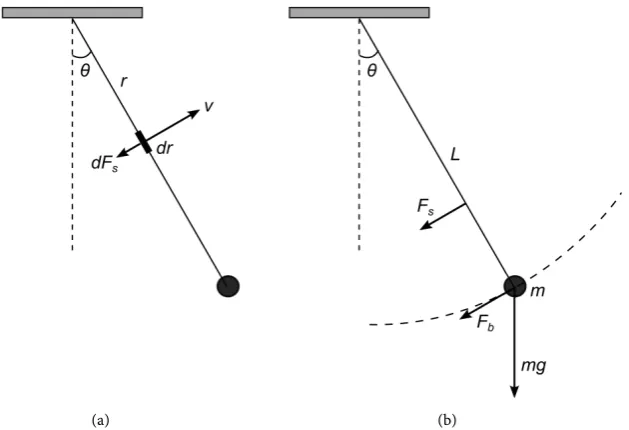
Consider an element of the string of a pendulum of length dr located at a dis-tance r from the support point and moving with velocity v, as shown in Fig-ure 1(a). The magnitude of the drag force on this element of the string dFs is proportional to the cross-sectional area of the element perpendicular to the di-rection of motion, D rd , where D is the diameter of the string. Furthermore, since this element is moving with small speeds, the drag force on it is propor-tional to its speed. Therefore, we have

[image:3.595.217.532.489.704.2]

(a) (b)

(4)

(

)

dFs =k D r vd (7)

where k is a constant. But since v=rθ, where θ is time derivative of

θ

,

we obtain

dFs=kD r rθ d (8)

Since this drag force is perpendicular to the string, its torque about the sup-port point is

2

dτs =r Fd s =kD rθ dr (9)

Integration of this equation over the length of the string, L, gives the total torque on the string,

3 2

0 d ₃

L s

kL D

kD r r

τ = θ

_∫

= θ₍₁₀₎

4. Equation of Motion

Derivation of the equation of motion of the simple pendulum with a linear drag force is trivial, however, we present it here for completeness of the discussion.

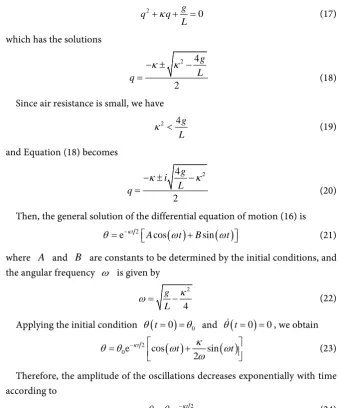
Figure 1(b) shows a simple pendulum with a bob of mass m and a total length L. The total drag force on the string and that on the bob of the pendulum are shown by Fs and Fb, respectively.

The equation of motion of the spring is

I

τ = α

∑

(11)

where all torques are calculated relative to the support point, α is the angular acceleration of the pendulum about this point, and 2

I =mL is the moment of

inertia of the pendulum about the support point (string has negligible mass). Using Figure 1(b), this equation reduces to

2

sin s b

mLθ= −mgL θ τ− −F L (12)

where τs is given by Equation (10). The third term on the right hand side of this equation is the torque caused by the force of air resistance on the bob of the pendulum, in which Fb is given by Equation (6), i.e.,

b

F =cv=cLθ (13)

Therefore, after some simplifications, Equation (12) becomes

sin 0

g L

θ κθ+ + θ = (14) where the damping constant κ is defined by

3

kLD c

m m

κ = + ₍₁₅₎

(5)

0 g L

θ κθ+ + θ = ₍₁₆₎

Equation (16) is a homogeneous second order linear differential equation with constant coefficients, whose solution is straightforward. We fist construct the auxiliary equation,

2 g ₀

q q

L κ

+ + = ₍₁₇₎

which has the solutions

2 4 2 g L q κ κ − ± −

= (18)

Since air resistance is small, we have

2 4g

L

κ < ₍₁₉₎

and Equation (18) becomes

2 4 2 g i L q κ κ − ± −

= ₍₂₀₎

Then, the general solution of the differential equation of motion (16) is

( )

2

eκt Acos t Bsin t

θ₌ − _ ω ₊ ω _

  (21)

where A and B are constants to be determined by the initial conditions, and the angular frequency ω is given by

2

4 g L

κ

ω= − (22)

Applying the initial condition θ

(

t=0

)

=θ0 and θ =

(

t 0

)

=0, we obtain

( )

2

0e cos sin

2

t

t t

κ κ

θ θ ω ω

ω

−  

= _ + _

  (23)

Therefore, the amplitude of the oscillations decreases exponentially with time according to

2 0e

t κ

θ θ₌ − ₍₂₄₎

5. Experiment and Results

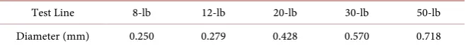
[image:5.595.201.540.150.559.2]

Throughout our experiment we used a steel ball of mass 485 g and diameter 50.9 mm as the bob of our simple pendulum. For string we used monofilament nylon fishing lines of various diameters. During the entire experiment, the total length of the pendulum was 261.4 cm, 258.9 of which was the length of the string. Al-though the thickness of each string was consistent throughout its length, we measure the diameter 8 times along its length while the string was under load.

Table 1 shows the mean diameters of the strings.

(6)

[image:6.595.210.539.89.122.2]

Table 1. Fishing test lines used as strings and their diameters.

Test Line 8-lb 12-lb 20-lb 30-lb 50-lb

Diameter (mm) 0.250 0.279 0.428 0.570 0.718

until the amplitude dropped to 10 cm. We note here that since the length of the string is about 259 cm, the linear amplitude of 30 cm corresponds to an angular amplitude of about 6.65_{. Then the error in using the approximation}_sin_{θ θ}_≈

in Equation (14) is only about 0.2%. We also note that the mass of the heaviest string used in our experiments (the 50-lb test line) was only 1.5 g, which is quite negligible compared to the mass of the bob.

Equation (24) may be written as

0

ln

2t

θ κ

θ  

= −  

  (25)

Therefore, a graph of ln

(

θ θ0

)

versus t should be a straight line with a slope of −κ 2. Figure 2 shows the results of our experiment for three of the

pendu-lums. We have not plotted all of them to avoid cluttering of the figure.

Figure 2 reveals two things. First, the fact that plots of ln

(

θ θ0

)

versus t are fairly straight lines in each case is indicative of the approximate correctness of the model used in this analysis. Second, since the same pendulum bob was used in all experiments, the distinct difference in the graphs for the lines with differ-ent diameters show that the string of the pendulum plays a significant role in the damping of the pendulum. If this was not the case and if the damping was al-most entirely due to the bob of the pendulum, the graphs should all coincide, or at least be indistinguishable from one another. Figure 2 also shows the linear least-squares fit to the data for each pendulum as a solid line. The slope of each line is −κ 2. From these slopes we have calculated the value of κ for each

string, which are shown in Table 2.

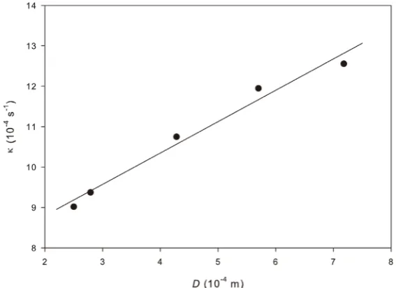
Because we used the same bob and the same string length in all experiments, according to Equation (15) the graph of the damping constant κ as a function of string diameter D should be a straight line. This is shown in Figure 3. As can be seen, the plot of κ vs D is, to a good approximation, a straight line. A least- squares analysis gives the following equation for the best line,

(

)

(

)

4

0.777 0.067 D 7.24 0.32 10

κ₌ _± ₊ _± _× − ₍₂₆₎

in which D is in meters and κ is in s−1_{. This line is also plotted in the figure.} The first term in Equation (26) is the contribution of the string of the pendu-lum to its damping (κS), and the second term is that of its bob (κB). Using the diameters of our strings and Equation (26), we can calculate these contributions in our experiments. The results are shown in Table 3.

6. Discussion

(7)

[image:7.595.234.515.70.270.2] [image:7.595.231.515.318.524.2]

Figure 2. Plots of amplitude versus time for the pendulums with different string diame-ters.

Figure 3. Damping constant as a function of string diameter.

Table 2. Damping constant for various strings tested.

[image:7.595.211.540.652.733.2]

String Diameter D (mm) 0.250 0.279 0.428 0.570 0.718 Damping Constant κ (10−4_s−1₎ _9.02 _9.37 _10.75 _11.95 _12.56

Table 3. Contributions to the damping constant of the pendulum from the string (κS)

and from the bob (κB).

String Diameter (mm) κS (10

−4_s−1₎

B

κ (10−4_s−1₎

0.250 9.18 7.24

0.279 9.41 7.24

0.428 10.57 7.24

0.570 11.67 7.24

(8)

0.367 m/s. With a room-temperature density of 1.204 kg/m3_[7]_{and an absolute}

or dynamic viscosity of 5

1.983 10× − Pa·s [8] for air, and the diameter of the bob

of 0.0509 m, Equation (5) gives a Reynolds number of 1134. Therefore, the linear model used for air resistance in this work is justified, which is further supported by the results in Figure 2 and Figure 3.

The results of Table 3 show that for all pendulums tested, the string plays a more significant role in damping than the bob, and this effect increases with the string diameter. This, however, is not surprising because even though the string of a simple pendulum may be very thin, its total frontal cross-sectional area can be comparable to that of the bob of the pendulum. For example, our string with diameter 0.718 mm and length 259 cm, has a frontal cross-sectional area of 18.6 cm2_{compared to 20.3 cm}2_{for the spherical bob. In addition, for Reynolds} num-ber of 1000, the drag coefficient of a sphere is 0.47 whereas that of a wire (a cir-cular cylinder with L D= ∞) perpendicular to the flow is 1.2 [9] [10]. A

com-bination of these factors results in a significant damping effect by the string of the pendulum.

7. Conclusion

In conclusion, the results of this investigation show that the string of a simple pendulum plays a significant role, and in some cases a more important role, in damping the pendulum than its bob. To the best of our knowledge, this effect has not been taken into account in the discussions of damping of pendulums in the literature.

Acknowledgements

This work was supported by a URAP grant from the University of Wisconsin- Parkside.

References

[1] Nelson, R.A. and Olsson, M.G. (1986) The Pendulum - Rich Physics from a Simple System. American Journal of Physics, 54, 112-121.https://doi.org/10.1119/1.14703

[2] Dunn, E.K. (2012) The Effect of String Drag on a Pendulum.

[3] Marion, J.B. and Thornton, S.T. (1995) Classical Dynamics of Particles and Systems, 4th Edition, Saunders, New York, 58-60.

[4] Mohazzabi, P. and Fields, J.C. (2004) High-Altitude Projectile Motion. Canadian

Journal of Physics, 82, 197-204.https://doi.org/10.1139/p04-001

[5] https://en.wikipedia.org/wiki/Drag_(physics)

[6] http://www.mne.psu.edu/cimbala/me325web_Spring_2012/Labs/Drag/intro.pdf

[7] http://www.engineeringtoolbox.com/air-density-specific-weight-d_600.html

[8] http://www.engineeringtoolbox.com/dynamic-absolute-kinematic-viscosity-d_412.

html

[9] Granger, R.A. (1995) Fluid Mechanics. Dover Publications Inc., New York, 400, 401, 781.

(9)

Coeffi-cient of a Cylinder Perpendicular to Water Flow by Numerical Simulation and Field Measurement. Ocean Engineering, 85, 93-99.

https://doi.org/10.1016/j.oceaneng.2014.04.028

Submit or recommend next manuscript to SCIRP and we will provide best service for you:

Accepting pre-submission inquiries through Email, Facebook, LinkedIn, Twitter, etc. A wide selection of journals (inclusive of 9 subjects, more than 200 journals)

Providing 24-hour high-quality service User-friendly online submission system Fair and swift peer-review system

Efficient typesetting and proofreading procedure

Display of the result of downloads and visits, as well as the number of cited articles Maximum dissemination of your research work

Submit your manuscript at: http://papersubmission.scirp.org/