http://www.scirp.org/journal/jcc ISSN Online: 2327-5227
ISSN Print: 2327-5219
Acceleration of Points to Convex Region
Correspondence Pose Estimation Algorithm
on GPUs for Real-Time Applications
Raghu Raj P. Kumar, Suresh S. Muknahallipatna, John E. McInroy
Department of Electrical and Computer Engineering, University of Wyoming, Laramie, USA
Abstract
In our previous work, a novel algorithm to perform robust pose estimation was presented. The pose was estimated using points on the object to regions on image correspondence. The laboratory experiments conducted in the pre-vious work showed that the accuracy of the estimated pose was over 99% for position and 84% for orientation estimations respectively. However, for larger objects, the algorithm requires a high number of points to achieve the same accuracy. The requirement of higher number of points makes the algorithm, computationally intensive resulting in the algorithm infeasible for real-time computer vision applications. In this paper, the algorithm is parallelized to run on NVIDIA GPUs. The results indicate that even for objects having more than 2000 points, the algorithm can estimate the pose in real time for each frame of high-resolution videos.
Keywords
Pose Estimation, Parallel Computing, GPU, CUDA, Real Time Image Processing
1. Introduction
In our previous work, a novel pose estimation algorithm based on points to re-gion correspondence was proposed in [1]. Given the points on an object and the convex regions in which the correspondent image points lie, the concrete values of position and orientation between the object and the camera are found based on points to regions correspondence. The unit quaternion representation of ro-tation matrix and convex Linear Matrix Inequalities (LMI) optimization
me-How to cite this paper: Kumar, R.R.P., Muk- nahallipatna, S.S. and McInroy, J.E. (2016) Acceleration of Points to Convex Region Cor- respondence Pose Estimation Algorithm on GPUs for Real-Time Applications. Journal of Computer and Communications, 4, 1-17.
http://dx.doi.org/10.4236/jcc.2016.417001
Received: October 31, 2016 Accepted: December 26, 2016 Published: December 29, 2016
Copyright © 2016 by authors and Scientific Research Publishing Inc. This work is licensed under the Creative Commons Attribution International License (CC BY 4.0).
http://creativecommons.org/licenses/by/4.0/
thods are used to estimate the pose. By loosening the requirement of precise point-to-point correspondence and using convex LMI formulations, the algo-rithm provided a more robust pose estimation method. While the pose estima-tion experiments yielded satisfactory results, the test cases considered were small objects with four points per object. While this may be reasonable for lab experi-ments, with the current high and ultra-high resolution images, larger objects are captured on images. Having a low number of points for larger objects, the pose estimation algorithm will have a low accuracy, as shown in [1]. It is also shown in [1] that for more points on a given object, the accuracy of the pose estimation increases. Moreover, some pose estimation based video processing applications require processing of larger objects in high-resolution images at high frame rates (300) in real-time, i.e., 300 high-resolution images have to be processed for an object with large number of points within a second to obtain the pose. Since, the serial execution time of the pose estimation algorithm is bound to the number of points, i.e., with a higher number of points, the execution time of the pose esti-mation algorithm also increases. This makes the pose estiesti-mation involving large objects with high accuracy, infeasible for real-time applications. Therefore, the algorithm requires further analysis to make it suitable for real-time applications.
The pose estimation algorithm, described in [1], is an iterative 2D search al-gorithm. The number of computations for the algorithm is dependent on two factors: a) number of points on objects, also known as markers and b) accuracy of the estimated pose. The number of computations within a single iteration is determined by the number of markers, i.e., the number of computations within each iteration increases linearly with an increase in the number of markers. The number of iterations is determined by the desired accuracy, i.e., the number of iterations increases non-linearly for higher order accuracy, as it is a 2D search. However, the iterations being independent of one another make concurrent ex-ecution of all iterations feasible. Since the number of concurrent iterations grows non-linearly with an increase in the desired accuracy, more execution cores are needed to maximize concurrency. Thus, the algorithm is well suited for General Purpose Computation on GPU (GPGPU) parallelization.
works.
The original work presented in [1] was written by one of our authors. The work has been used in [2] and also has been acknowledged as a highly accurate pose estimation algorithm in [3][4]. However, no effort has been made to paral-lelize the algorithm described in [1]. There are several real-time suitable pose es-timation algorithms published in the year 2015 alone, [5]-[11] to mention a few. However, these algorithms have limitations based on their approach. Pose esti-mation described in [5][6][7][8] require a database of objects. The limitation of using database centered pose estimation is the overhead involved in creating a useful, open source and widely accepted database. Moreover, the pose estimation application would be limited to the objects in the database. The pose estimation algorithm described in [8] [9] exploit certain features for a given object. The usage of such algorithm is limited to certain objects, thereby limiting its applica-tion. The pose estimation described in [10] requires special cameras. The cam-eras are an additional cost, and may not be feasible to use in different kinds of application. On the contrary, the algorithm described in [1] is generic pose esti-mation algorithm with high accuracy, i.e., it does not require a database or ex-ploit certain features of an object or use special cameras. In comparison to other generic and highly accurate pose estimation algorithms, it estimates pose with-out subjecting the estimation to local minima or divergence [1].
un-manned air vehicles (UAV) for takeoff and landings. The authors in [14] per-form a field evaluation using low end GPUs such as Jetson TK1. It is observed that pose estimation takes under 25 milliseconds for standard 640 × 480 images. Though the algorithm has good performance, especially considering that the si-mulations were carried out on a low-end GPU, it is explicitly used for UAV.
The purpose of our work is to extend the work in [1]. Parallelizing the algo-rithm in [1] would help us build a highly accurate, robust, real-time feasible and scalable algorithm, which would make our parallel version of pose estimation algorithm unique, with respect to all other algorithms that have only few, but not all, of the above mentioned features.
This paper is organized as follows: Section 2 describes an implementation of the algorithm provided in [1]. Section 3 provides the optimization design. In Section 4, the performance of our parallel implementation is compared with se-quential execution and a parallel implementation of the continuous 8-point pose estimation algorithm. We conclude the paper by summarizing our findings.
2. Pose Estimation Algorithm
The implementation description of the pose estimation algorithm introduced in
[1] henceforth known as the optimal position estimation algorithm (OPEA) is provided in this section. The following assumptions for the implementation are made:
a) Monocular pose estimation is considered.
b) There is a relative motion between the camera and object. c) There are at least four markers per object.
d) Camera captures images in the form of video frames, with at least 24 frames per second (fps). The fps is assumed to increase with an increase in the rate of relative motion between the camera and the object.
e) It is a continuous pose
( )
ω,v estimation, where, ω= ωx ωy ωzT isthe angular velocity relative to the camera and object, T x y z
v= v v v is the
translational velocity relative to the camera and the object
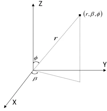
f) The velocity, v, is measured in spherical coordinates. Spherical coordinates
(
r, ,β ϕ)
are represented by radial distance (r), azimuthal angle( )
β
and polarangle
( )
ϕ
as shown in Figure 1. By assuming π π, π π2 β 2 2 ϕ 2
− ≤ ≤ − ≤ ≤
and r = 1, an iterative search can be performed with ease and then scaled by a factor of radial distance.
Since OPEA is an iterative 2D search algorithm, it explores a 2D space for all possible values of the pose of v and ω. The search begins by assuming a value of v, where v in spherical coordinates is given by v=
[
sin cosϕ β sin sinϕ β cosϕ]
,and 1, π π, π π
2 2 2 2
r= − ≤ ≤
β
− ≤ ≤ϕ
. The magnitude of v is inherently ambi-(
r,β,φ)
r
β
φ
Z
Y
[image:5.595.277.462.74.265.2]X
Figure 1. Spherical coordinate system representation.
= 1. For each assumption of v, a corresponding ω is calculated. The error in
( )
ω,v pair estimation is calculated by re-projecting all the markers of theob-ject. The error is quantized and compared across all values of
( )
ω,v . The( )
ω,v providing the least error and positive depths for all markers is selected asthe pose. Since the value determining v have boundary conditions π π,
2 β 2
− ≤ ≤
π π
2
ϕ
2− ≤ ≤ , the increment intervals of β and
ϕ
determine the accuracy of the pose estimated, i.e., the smaller the incremental value of β andϕ
, the greater the accuracy of( )
ω,v .Consider two images taken from a single camera with relative velocity be-tween the image and the object. Let the image coordinates of markers on the first image be xl, where
[
]
T 1
x= x y and
l
=
4,
,
m
f andm
f represents thenumber of markers per image frame. Let the difference between the markers’ positions on the second frame from the first frame be represented by xl, where
[
]
T1 2 0
x= x x . Unit vectors for xl and xl are calculated using: l
l l
x u
x
= (1)
(
T)
ll l l
l
x
u I u u
x
= −
(2)
where I represents an identity matrix and T l
u represents the transpose of ul.
Once a value of v is assumed, a corresponding value for ω is calculated as fol-lows:
1
C B
ω= − − (3)
2 T 2 1
ˆ ˆ
j
m
l l l
C u vv u
=
2 T 1
ˆ ˆ
j
m
l l l l
B u vv u u
=
=
∑
(5)3 2 3 1 2 1 0 ˆ 0 0 u u
u u u
u u − = − − (6)
1 2 3
u= u u u (7)
The difference
(
i ˆ i)
u −ωu provides the error measurement in ω. We obtain
the cross product of this difference with u to obtain a perpendicular vector, rep-resentative of the error in estimating pose. This process removes the depth of all points from the equations. A single scalar value error (J) for all markers of an object, indicating the error in estimating
( )
ω,v is calculated as follows:(
)
(
)
T1
ˆ ˆ
ˆ ˆ
j
m
s l l l l l l
l
Q u u ωu u u ωu
=
=
∑
− − (8)T s
J=v Q v (9)
Thus, the plot of J versus
(
β ϕ,)
, selected for v, provides a surface. The lowestpoints
(
β ϕ,)
with respect to J on the surface show possible( )
ω,v values withlowest errors. Similar to other pose estimations, depth constraints dictated by the epipolar geometry helps in selecting the right pose. The depth (d) constraint for each marker is calculated as follows:
(
)
T ˆl l l
d = u −ωu v (10)
If the depth of all points has the positive numerical sign and the value of J
corresponding to the same
( )
ω,v is minimal, then( )
ω,v is taken as the pose.If the depth of all points has the negative numerical sign and the value of J cor-responding to the same
( )
ω,v is minimal, then the pose is taken to be(
ω −, v)
.3. Parallelization of OPEA
We begin this section by analyzing the calculations in OPEA. The analysis is split into two phases. The first phase analyzes code refactoring of OPEA to suit parallelization. However, the refactored code can be used as a sequential or pa-rallel code. The second phase analyzes the data reorganization and code for a parallel implementation of the refactored code, to match the GPU architecture.
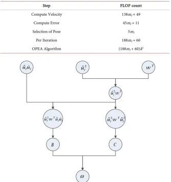
The first phase of analysis begins by splitting the calculations in OPEA into three steps. Equations (1)-(5) are taken to be the “compute velocity” step. Equa-tions (8), (9) are taken to be “compute error” step. Lastly, Equation (10) is taken to be the “selection of pose” step. If the total number of iterations in each di-mension is represented by k, Table 1 shows the number of floating point of op-erations (FLOP) for each step.
Hence the execution time of OPEA increases linearly with an increase in mf
Table 1 also shows that the compute velocity step has the maximum FLOP count in the computation phase. Analyzing Equations (1)-(7), the dependency of variables for the compute velocity step is provided in Figure 2. Clearly, the compute velocity step in OPEA has varied data dependencies, which can be se-parated as:
a) v dependent computations b) v independent computations
Since only v dependent computations are needed inside the iteration, the v
independent computations can be pcomputed outside the iterations, thus re-ducing the total FLOP count of OPEA.
We now provide an advanced version of OPEA, referred to as AOPEA, which refactors code to suit parallelization better. To facilitate code refactorization, we introduce two new operations
a) Stackoperation: Convert 3 × 3 symmetric matrix elements to a vector. b) Unstackoperation: Convert 6 × 1 vector into 3 × 3 symmetric matrix.
Table 1. FLOP Count Split-up for OPEA Algorithm.
Step FLOP count
Compute Velocity 138mf + 49
Compute Error 45mf + 11
Selection of Pose 5mf
Per Iteration 188mf + 60
OPEA Algorithm (188mf + 60)k2
2 ˆl
u
l lu
uˆ T
vv
T lvv
uˆ2
2
2 ˆ
ˆ T l
lvv u
u
C
l l T lvv uu
uˆ2 ˆ
B
ω
1 2 3
2 4 5 1 2 3 4 5 6
3 5 6
stack
unstack
s s s
s s s s s s s s s
s s s
→ ←
The computation of B, C and Qs are performed in two parts. The v indepen-dent computations, computed only once for a given set of markers, represented
by
B C Q
p,
ps,
sp, and intermediary result variable Mp are calculated as shownbe-low:
T
1 1
1 2 2 1
1 3 3 1
1 2 2
2 3 3 2
3 3
f
l l
l l l l
m l l l l
p l l
l
l l l l
l l c c c c c B c c c c µ µ µ µ µ µ µ µ µ = + + = +
∑
(11)[
]
1 1 2 1 3 10 1 0
0 0 1
0 0 1
f f f m l l m s l p l m l l u C u u = = = =
∑
∑
∑
(12)( )
(
2)
1 ˆ ˆ
f
m j
sp l l l j l
Q u u u
=
=
∑
(13)( )( )
T1
ˆ ˆ
f
m
p l l l l l
M u u u u
=
=
∑
(14)where,
( )
ˆ
ll l
c
=
u u
(15) 21 2 3
ˆ l l l
l
u = µ µ µ (16)
T
1 1
1 2 2 1
1 3 3 1
2 2
2 3 3 2
3 3
l l j
l l l l
j j
l l l l
l j j
j l l
j
l l l l
j j
l l j
u
µ µ
µ µ µ µ
µ µ µ µ
µ µ
µ µ µ µ
µ µ + + = + (17)
where l j
c
represents the thj element of the vector cl and µ µ µ1, 2, 3 are
vectors. The v dependent computations, which are performed for all iterations, to complete the calculations of B, C and Qs are provided below:
S p
B
=
B v
(18)(
)
unstack s S p
T
s p
Q
=
M
+ +
N
N
+
C
(20)where,
( )
T stack Sv = vv (21)
[
s1 s2 s3]
N= Q ω Q ω Q ω (22)
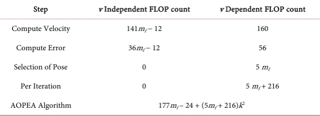
The new FLOP count for the AOPEA is provided in Table 2. In comparison with OPEA, the number of computations is observed to be significantly lower.
The steps for selection of pose, discussed in Equation (10), can be skipped if J
is greater than an already computed minimum value. Hence, neglecting the FLOP count for the same, the total FLOP count for AOPEA is 177mf + 216k2 –
24. The separation of mf and k2 computational steps facilitates an increase in
ex-ecution time exclusive to either the number of markers or accuracy. For exam-ple, a real-time application requiring higher accuracy can have lower mf and high k value, whereas a real-time application requiring higher mf can have low k
iteration count. In both cases, only the computations relevant to each are in-creased.
To reduce the overhead of iterations further; the v dependent computations are performed twice-first with coarse accuracy with high increments for each iteration, and second with finer accuracy with smaller increments for each itera-tion. Coarse accuracy iterations, having smaller values of k, provide a coarse es-timation of
( )
ω,v which helps in limiting the search to a smaller interval. Thesecond round of v dependent computations are performed with finer accuracy values for a much smaller interval around the coarse estimated
( )
ω,v . Thesemodifications result in refactoring the OPEA code to AOPEA algorithm along with refactored code. Thus, this reduces the total number of iterations per-formed significantly. The increment values for the coarser and finer iterations are dependent on the application. The AOPEA can be implemented either as a sequential or parallel algorithm.
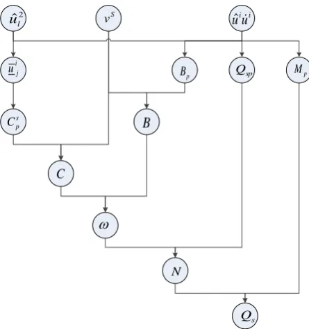
[image:9.595.209.539.585.705.2]The second phase of analysis looks at the implementation of AOPEA as a pa-rallel algorithm. It begins with looking at data reusability for the algorithm. Fig-ure 3 shows how some of the computed data variables can repeatedly be used.
Table 2. FLOP count Split-up for AOPEA algorithm.
Step v Independent FLOP count v Dependent FLOP count
Compute Velocity 141mf − 12 160
Compute Error 36mf − 12 56
Selection of Pose 0 5 mf
Per Iteration 0 5 mf + 216
2 ˆl
u S
v i i
u
u
ˆ
i j
u
s p
C
p
B Qsp Mp
B
C
ω
N
s
[image:10.595.260.483.68.306.2]Q
Figure 3. AOPEA data reusability.
For the v independent computations, we arrange the data into two matrices such that one matrix-matrix multiplication provides the results for BP, Qspand
mp. We perform a global synchronization after vindependent computations are completed. The results thus obtained are re-arranged into a single matrix, and distributed (data) to many-cores on GPUs, known as streaming processors. This arrangement facilitates coalesced memory access for all matrix or vector multip-lications and additions involved. Coalesced memory access on GPUs, are shown to provide better performance in [15]. Since iterations are mutually exclusive, we can assign one iteration search to a single streaming processor on the GPU. Apart from separating the iterations, GPU-based code optimizations as shown in
[15] are performed on the code for maximum performance.
4. Results
In this section, we analyze the effectiveness of AOPEA, its parallelization, and scalability. To analyze AOPEA, first, we compare the execution time of sequen-tial implementation of AOPEA with a reference pose estimation algorithm, and sequential OPEA algorithm. For the reference pose estimation, we use the con-tinuous pose estimation algorithm (CPEA). Second, we look at the execution time of parallel implementations of CPEA, OPEA, and AOPEA parallelized us-ing standard parallel libraries. Lastly, we look at the execution time of our paral-lel implementation of AOPEA, analyzing its scalability.
Matlab’soriginal core has been developed from LINPACK and EISPACK [16]. LINPACK and EISPACK have proven to be computationally effective ways to solve linear algebra problems [17]. Hence we use this software to obtain the ref-erence time for sequential programs.
For parallel program execution, the CPU is equipped with a NVIDIA Tesla C2075 card. The card is equipped with 448 cores and 6GB of memory for general computations. Though K20x and K40m cards seem to be a good option for GPU parallelization, we limit ourselves to a low-cost GPU such as C2075. For the de-velopment of parallel AOPEA implementation, NVIDIA’s CUDA 6.0 integrated with Microsoft Visual 2015 via NSight was used. For developing parallel CPEA, OPEA and AOPEA code using standard libraries, cuBLAS library package was used. cuBLAS library package is an accelerated Basic Linear Algebra Subpro-grams (BLAS) library provided by NVIDIA for GPUs. A combination of APIs available in the cuBLAS package is used to perform the operations in CPEA, OPEA, and AOPEA. Lastly, for profiling NVIDIA’s Visual Profiler, NVVP, com- patible with CUDA 6.0 and Microsoft Visual 2015 was used to profile the code.
For the purpose of this paper, we use execution time as a measure of perfor-mance. Low execution time is considered to be better. Each implementation of an algorithm (CPEA, OPEA or AOPEA) for a given marker size and accuracy is considered as one simulation and the execution time is collected. Each simula-tion is executed one thousand times and an average execusimula-tion time (AET)is computed. The standard deviation of AET for all simulations was observed to be under 3%. Each simulation has been verified by reconstructing objects in images. Data, for verification of algorithms, is taken from videos under indoor computer lab conditions using 60 fps at 1080 p resolution. The number of markers for si-mulations is varied to study the scalability of the algorithms, i.e., we choose
5 6 11
2 , 2 , , 2 f
m = . For all simulations, the accuracy is assumed to be 0.01
ra-dians which satisfies the accuracy required for 3D re-projection for real-time ap-plications. For AOPEA, the accuracy for the coarse resolution is taken to be 0.15
radians, and 0.01 radians for finer resolution. The interval for the finer search is taken to be twice the coarse resolution.
Table 3 shows the sequential AET of CPEA, OPEA and AOPEA algorithms for a different number of markers per frame. For smaller mf, the CPEA has lower AET, whereas, for larger mf, the CPEA has a non-linear increase in AET. This is due to the computations in CPEA being
( )
( )
3f
O m . Hence for small mf, AET
for CPEA is low and grows exponentially as mf increases. The computations of OPEA, as seen in Table 1, are
(
2)
f
O m k . Hence, the AET for OPEA is
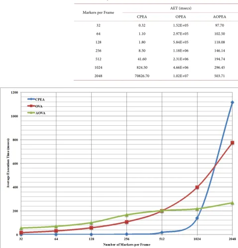
Next, we look at the parallel implementation of CPEA, OPEA and AOPEA, implemented using cuBLAS library API calls. The results, which include the data transfer time between CPU and GPU, are presented in Figure 4. The CPEA, af-ter parallelization, shows reduced AET in comparison to sequential AET, showing
Table 3. Average execution time for sequential CPEA, OPEA, and AOPEA algorithms for different markers per frame.
Markers per Frame AET (msecs)
CPEA OPEA AOPEA
32 0.32 1.52E+05 97.70
64 1.10 2.97E+05 102.50
128 1.80 5.84E+05 118.08
256 8.50 1.18E+06 146.14
512 41.60 2.31E+06 194.74
1024 824.50 4.66E+06 296.45
2048 70826.70 1.02E+07 503.71
good scaling till 512 mf. This is because CPEA has sufficient parallelism in its code. However, for mf > 512 the profiler indicated occupation of all cores on the GPU. This forces fragments of code in the queue to wait till cores become idle serializing the execution, increasing the AET. In the case of OPEA, the algorithm is embarrassingly parallel with respect to iterations i.e., the number of iterations is more than 90,000 and independent of one another. Hence, the problem has enough workload for GPUs even for low mf. The profilers indicate that the GPU cores are completely occupied. But, as mf increases, due to the lack of idle GPU cores, more code execution is serialized leading to higher AET. In case of AOPEA, with lower computations than CPEA and OPEA and increasing linearly with increase in mf, the AET shows small increments for every doubling of mf. Due to the separation of v dependent and independent computations in AOPEA, the data needs to be re-arranged after completing the v independent computa-tions. This forces additional data transfers between CPU and GPU. For low val-ues of mf, the AET is limited by the overhead of data transfers between CPU and GPU. In fact, the data transfers contribute to nearly 90% of AET for all values of
[image:13.595.57.540.367.688.2]mf. However, despite overhead of data transfer time, AOPEA has the best AET for higher values of mf.
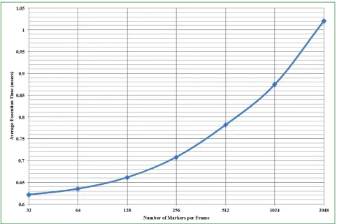
Figure 5 shows the AET of our version of AOPEA for different mf values. Due
to a single data transfer between CPU and GPU in each direction, and highly op-timized code, the AET is found to be just over a millisecond for 2048 markers. The implementation also shows good scalability even at 2048 markers, unlike
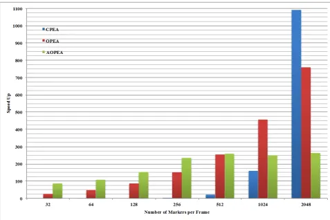
Figure 4 i.e., with an increase in markers there is a linear increase of AET. To better compare the performance of our version of parallel AOPEA, Figure 6
provides the speed up of our parallel implementation of AOPEA with CPEA, OPEA and AOPEA implemented using cuBLAS library calls. In case of CPEA, the speed up exponentially increases, especially for higher mf. In case of OPEA, we observe a linear speed up with an increase in markers. Whereas for AOPEA, the speed up saturates at about 250×. The low AET and good scalability of our parallel implementation of AOPEA indicate its suit ability for real-time applica-tions.
[image:14.595.60.538.366.684.2]Though our version of pose estimation shows low AET, using it for real-time applications may have higher AET. This is because real-time applications com-bine pose estimation with tracking of markers. This would involve additional overheads. For example, real-time applications would use a video, where each frame is considered as an image. The image from the camera needs to be trans-ferred to CPU, and then to the GPU. The image may also need to be pre- processed to obtain distinct position of markers. In order to show that our parallel
implementation can be used for real time applications, we conducted a lab expe-riment. A 1000 fps high-resolution camera was used to capture a video tracking 32 markers. The position of the 32 markers were pre-calculated, but fed to the pose estimation algorithm in real time on a per image basis. Simulations for dif-ferent image resolutions were conducted, where each image obtained from the camera, was copied to CPU, transferred to GPU, converted from Red-Green- Blue format to gray-scale format, and then pose was estimated. Using simula-tions’ AET, the supported fps that our pose estimation algorithm could process, was calculated.
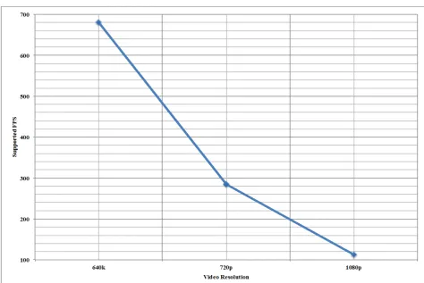
Figure 7 shows the supported fps by our parallel implementation of AOPEA for 640 × 480 (640 k), 1280 × 720 (720 p) and 1920 × 1080 (1080 p) resolution videos. For 640 k videos, real-time applications using 600 fps can use our parallel implementation with ease since our implementation supports 681 fps. However, for 720 p and 1080 p, due to the large amount of data, we observe a sharp de-crease in supported fps. For 720 p, our parallel implementation of AOPEA sup-ports 285 fps, whereas for 1080 p, it supsup-ports 112 fps.
5. Conclusions
We have modified the algorithm provided in [1] to meet the performance
requirements of real-time applications. An analysis of the implementation indi-cated that there was a) redundancy in computations and b) data and code or-ganization un-fitting for GPU architectures. We modified the implementation, to suit parallelization on GPU architectures, in two phases: first, refactoring the algorithm to have lesser number of operations and enhanced parallelism, and secondly, optimizing the data and code to obtain better parallelism for GPU ar-chitectures. We compared the effectiveness of our algorithm AOPEA, with CPEA and OPEA, for sequential and parallel implementations. For sequential implementation, AOPEA performed much better than its predecessor algorithm OPEA. However, for lower markers per frame, CPEA performed better than AOPEA whereas for higher markers per frame AOPEA performed better than CPEA. To understand the effectiveness of our parallel implementations, CPEA, OPEA and AOPEA were parallelized using the cuBLAS library and compared with our parallel implementation. The results showed that our parallel mentation of AOPEA has lowest execution time. Moreover, our parallel imple-mentation also showed good scalability of performance with an increasing num- ber of markers per frame. Moreover, a lab simulation of a real-time application indicated that our parallel implementation of AOPEA supports at least 100 fps even for high-resolution videos. Hence, our parallel implementation of AOPEA could be implemented on GPUs for real-time applications using high-resolution frames with a high number of markers per frame.
For our future work, we plan on pursuing two additions to the AOPEA: a) multi-GPU implementation of the algorithm for images from 3 - 4 cameras, and b) integrating our AOPEA and multi-GPU AOPEA algorithm with a tracking algorithm.
References
[1] McInroy, J.E. and Qi, Z. (2008)A Novel Pose Estimation Algorithm Based on Points to Regions Correspondence. Journal of Mathematical Imaging and Vision, 30, 195- 207. https://doi.org/10.1007/s10851-007-0045-2
[2] Qiao, B., Tang, S., Ma, K. and Liu, Z. (2013) Relative Position and Attitude Estima-tion of Spacecrafts Based on Dual Quaternion for Rendezvous and Docking. Acta Astronautica, 91, 237-244. https://doi.org/10.1016/j.actaastro.2013.06.022
[3] Yang, D., Liu, Z., Sun, F., Zhang, J., Liu, H. and Wang, S. (2014) Recursive Depth Parametrization of Monocular Visual Navigation: Observability Analysis and Per-formance Evaluation. Information Sciences, 287, 38-49.
https://doi.org/10.1016/j.ins.2014.07.025
[4] Yang, D., Sun, F., Wang, S. and Zhang, J. (2014) Simultaneous Estimation of Ego- Motion and Vehicle Distance by Using a Monocular Camera. Science China Infor-mation Sciences, 57, 1-10. https://doi.org/10.1007/s11432-013-4884-8
[5] Whelan, T., Kaess, M., Johannsson, H., Fallon, M., Leonard, J.J. and McDonald, J. (2015) Real-Time Large-Scale Dense RGB-D SLAM with Volumetric Fusion. The International Journal of Robotics Research, 34, 598-626.
[6] Gálvez-López, D., Salas, M., Tardós, J.D. and Montiel, J.M.M. (2016) Real-Time Monocular Object Slam. Robotics and Autonomous Systems, 75, 435-449. https://doi.org/10.1016/j.robot.2015.08.009
[7] Lim, H., Sinha, S.N., Cohen, M.F., Uyttendaele, M. and Kim, H.J. (2015) Real-Time Monocular Image-Based 6-DoF Localization. The International Journal of Robotics Research, 34, 476-492. https://doi.org/10.1177/0278364914561101
[8] Tagliasacchi, A., Schröder, M., Tkach, A., Bouaziz, S., Botsch, M. and Pauly, M. (2015) Robust Articulated-ICP for Real-Time Hand Tracking. Computer Graphics Forum,34, 101-114. https://doi.org/10.1111/cgf.12700
[9] Rymut, B. and Kwolek, B. (2015) Real-Time Multiview Human Pose Tracking Us-ing Graphics ProcessUs-ing Unit-Accelerated Particle Swarm Optimization. Concur-rency and Computation: Practice and Experience, 27, 1551-1563.
https://doi.org/10.1002/cpe.3329
[10] Sun, K., Heß, R., Xu, Z. and Schilling, K. (2015) Real-Time Robust Six Degrees of Freedom Object Pose Estimation with a Time-of-Flight Camera and a Color Cam-era. Journal of Field Robotics, 32, 61-84. https://doi.org/10.1002/rob.21519
[11] Poirson, P., Ammirato, P., Fu, C.Y., Liu, W., Kosecka, J. and Berg, A.C. (2016) Fast Single Shot Detection and Pose Estimation.
[12] Zabulis, X., Lourakis, M.I. and Koutlemanis, P. (2016) Correspondence-Free Pose Estimation for 3D Objects from Noisy Depth Data. The Visual Computer, 1-19. https://doi.org/10.1007/s00371-016-1326-9
[13] Haque, A., Peng, B., Luo, Z., Alahi, A., Yeung, S. and Fei-Fei, L. (2016) Towards Viewpoint Invariant 3D Human Pose Estimation. 14th European Conference on Computer Vision, Amsterdam, 11-14 October 2016, 160-177.
https://doi.org/10.1007/978-3-319-46448-0_10
[14] Benini, A., Rutherford, M.J. and Valavanis, K.P. (2016) Real-Time, GPU-Based Pose Estimation of a UAV for Autonomous Takeoff and Landing. IEEE International Conference on Robotics and Automation, Stockholm, 16-21 May 2016, 3463-3470. https://doi.org/10.1109/icra.2016.7487525
[15] Ryoo, S., Rodrigues, C.I., Baghsorkhi, S.S., Stone, S.S., Kirk, D.B. and Hwu, W.M.W. (2008) Optimization Principles and Application Performance Evaluation of a Mul-tithreaded GPU Using CUDA. Proceedings of the 13th ACM SIGPLAN Symposium on Principles and Practice of Parallel Programming, Salt Lake City, 20-23 February 2008, 73-82. https://doi.org/10.1145/1345206.1345220
[16] Ramaswamy, S., Hodges, E.W. and Banerjee, P. (1996) Compiling Matlab Programs to ScaLAPACK: Exploiting Task and Data Parallelism. Proceedings of the 10th In-ternational Parallel Processing Symposium, Honolulu, 15-19 April 1996, 613-619. https://doi.org/10.1109/ipps.1996.508120
Submit or recommend next manuscript to SCIRP and we will provide best service for you:
Accepting pre-submission inquiries through Email, Facebook, LinkedIn, Twitter, etc. A wide selection of journals (inclusive of 9 subjects, more than 200 journals)
Providing 24-hour high-quality service User-friendly online submission system Fair and swift peer-review system
Efficient typesetting and proofreading procedure
Display of the result of downloads and visits, as well as the number of cited articles Maximum dissemination of your research work
Submit your manuscript at: http://papersubmission.scirp.org/