A Simple Interest Rate Model with Unobserved Components: The Role of the Interbank Reference Rate

(1)

Munich Personal RePEc Archive

A Simple Interest Rate Model with

Unobserved Components: The Role of

the Interbank Reference Rate

Muto, Ichiro

11 December 2012

Online at

https://mpra.ub.uni-muenchen.de/43220/

(2)

A Simple Interest Rate Model with Unobserved

Components: The Role of the Interbank Reference Rate

Ichiro Muto

y

December 2012

Abstract

In this study, we theoretically investigate the potential role of the reference rate in stabilizing or destabilizing an interbank market with an environment where individual banks cannot fully identify the nature of underlying shocks a¤ecting their interbank transactions. We show that a noise-free reference rate based on a su¢cient number of sample transactions can help to make the market interest rate less volatile, whereas the stabilizing e¤ects of the reference rate are signi…cantly reduced if the reported interest rates contain some noisy components. Nevertheless, by increasing the number of sample transactions re‡ected in the reference rate, the adverse e¤ects of the noise can be mitigated (or eliminated) provided the noise is idiosyncratic to individual transactions. However, if the noise is common to multiple transactions, then the adverse e¤ects of the noisy reference rate cannot be reduced simply by increasing the number of sample transactions. This suggests that the noise in the interest rates reported by just a few of large banks can end up making the entire market more volatile, thereby impairing the transmission mechanism of monetary policy.

JEL Classi…cation: E43, E44, G14

Keywords: Interbank Market; Reference Rate; LIBOR; Imperfect Information; Financial Stability; Transmission Mechanism of Monetary Policy.

The author is grateful to Koichiro Kamada, Kosuke Aoki, Teruyoshi Kobayashi, Takeshi Kimura, Hibiki Ichiue, Kenji Nishizaki, Takashi Nagahata, Nao Sudo, and Takemasa Oda for their helpful advice and comments. The views expressed in this paper are those of the author and do not necessarily re‡ect the o¢cial views of the Bank of Japan.

(3)

1 Introduction

The role of the reference rate in interbank markets has become a major concern for various agents active in …nancial markets in light of the recent LIBOR manipulation problem. Policymakers the world over are already debating possible measures to the reliability and e¢cacy of interbank refer-ence rates, but numerous issues have yet to be fully addressed by the existing literature, including (i) the mechanism by which the reference rate contributes to …nancial markets stabilization, (ii) conditions under which the reference rate might actually serve to destabilize …nancial markets, (iii) the speci…c properties that might allow a reference rate to help stabilize …nancial markets and thereby enhance the e¤ectiveness of monetary policy.

In this study, we theoretically investigate the potential role of the reference rate in stabilizing or destabilizing …nancial markets, which is evaluated in terms of the volatility of interbank interest rates. To this end, we introduce a simple interest rate model in which individual banks cannot fully identify the nature of the underlying shocks that a¤ect individual interbank transactions. More speci…cally, we assume that the banks engaged in individual interbank transactions cannot distin-guish whether the underlying shocks are speci…c to individual transactions or broadly in‡uential to the entire interbank market.

This kind of imperfect information environment is analogous to the famous island economy model developed by Phelps (1970) and Lucas (1972, 1973) in the context of the output-in‡ation tradeo¤s and the e¤ectiveness of monetary policy. We believe that our setup is useful to gain insights into the potential role of the reference rate, since its most fundamental one is considered to be the information it provides to individual banks. That is, the reference rate should ideally inform individual banks of the aggregate …nancial conditions that exist throughout the entire interbank market, thereby helping these banks to set more appropriate interest rates in individual interbank transactions and making the average interbank interest rate less volatile. Our framework allows for the reference rate to play this sort of role, and also enables us to investigate how the existence of distortions (or noise) in the reference rate can have a destabilizing impact.1

Our analysis based on a simple model of the interbank market contributes to the academic literature by shedding light on the essential role of the reference rate in …nancial market stability.2;3

However, our potential contribution is by no means limited to the issue of …nancial stability. A

1_{Our study is similar to the argument of Morris and Shin (2002) in the sense that market participants react to the}

noise included in the common signals. However, our framework is simpler than theirs because we do not introduce any strategic complementarity among market participants.

2_{Although our theoretical setup is new to the literature, a previous empirical study provided by Angelini, Nobili,}

Picillo (2011), who investigate interest rate determinants for individual transactions in the Italian interbank market, does present an empirical model in which individual interbank interest rates are a¤ected by both bank-speci…c factors and aggregate factors.

3_{Some previous studies, such as Freixas and Holthausen (2004) and Heider, Hoerova, and Holthausen (2009),}

(4)

properly functioning interbank market is vital to the e¤ectiveness of monetary policy transmission. In our model, the market interest rate should be perfectly correlated with the central bank’s interest rate if information is perfect, while the average interest rate in the interbank market will tend to deviate from the policy rate in an imperfect information world. We show that the existence of a noise-free reference rate based on a su¢cient number of sample transactions leads to an increased correlation between the interbank rate and the policy rate, thereby enhancing the e¤ectiveness of monetary policy transmission.

This study is obviously not an exhaustive investigation of topics relating to the reference rate. For example, the recent LIBOR problem highlights a possible incentive for banks to manipulate interest rates through their reporting. Our analysis assumes that noise in the reported interest rates is purely exogenous, leaving the possibility of endogenous noise (manipulation) to other studies such as Ewerhart et al. (2007).4 _{In addition, we have limited our focus to interbank markets.}

From a macroeconomic perspective, the impact of interbank market stability (or instability) on the aggregate economy, through the linkage between the interbank market and other macroeconomic activities, should be examined in the context of dynamic general equilibrium (DSGE) models, as suggested by Woodford (2010).5 _{The rami…cations of the spread between the interbank interest}

rates and the policy rate for monetary policymakers are also worthy of investigation. Finally, our analysis does not consider potential problems arising from the “o¤shore” nature of LIBOR. Reasons why o¤shore rates are used as the reference rates in many developed countries are brie‡y explained in some studies, but a deeper analysis of potential pitfalls should be the subject of future research.6

The remainder of this study is organized as follows. In Section 2, we present our simple interest rate model with unobserved components. In Section 3, we provide a benchmark analysis under the assumption that individual banks can observe each component separately. In Section 4, we examine how the results di¤er when individual banks are unable to observe each component separately. In Section 5, we investigate the role of the reference rate in stabilizing the market interest rate. In Section 6, we examine the implications of the noise in the reference rate. In Section 7, we present some numerical examples to illustrate the role of the reference rate and the implications of noise in the reference rate. Section 8 concludes our analysis.

4_{Empirical studies examining the possibility of LIBOR manipulation during global …nancial crisis include}

Gyn-telberg and Wooldridge (2008), Abrantes-Metz et al. (2012), and Kuo, Skeie, and Vickery (2012).

5_{Sudo (2012) explores the roles played by the interbank reference rate in business cycle ‡uctuations using a DSGE}

model with credit frictions, which is developed and estimated by Muto, Sudo, and Yoneyama (2012).

6_{Gyntelberg and Wooldridge (2008) present some potential reasons why the o¤shore rate is preferred as the}

(5)

2 Model

We consider a situation in which each bank cannot fully identify the sources of underlying shocks that have an in‡uence on individual interbank transactions. Suppose that there are an in…nite number of transactions (indexed by j = 1; ;1_{) in an interbank market. The interest rate for}

thejth transaction is determined by the following two equations:

i_tj =ip_t+E_tj(!j_t _t); (1)

!j_t = _t+"j_t; (2)

where ij_t is the interest rate for the jth transaction and ip_t is the policy interest rate. !j_t is the fundamental factor in‡uencing on the jth transaction (such as funding liquidity and counterparty credit risk), _t is the aggregate component of!j_t, and"j_t is the individual component of!j_t.7

(1) indicates that the banks in the jth transaction set the interest rate by adjusting the pol-icy interest rate using their estimate of the deviation of factor !j_t from its aggregate component: E_tj(!j_t _t).8;9 _{(2) indicates that the fundamental factor for the}_{jth transaction consists of a shock}

in‡uencing on the entire interbank market ( _t) and a shock speci…c to the jth transaction ("j_t). These equations capture a situation in which the banks identify the individual shocks in the jth transaction and then take account of these shocks in determining their individual interest rate.

This kind of framework with imperfect information is analogous to the famous island economy model introduced by Phelps (1970) and Lucas (1972, 1973) in the context of the output-in‡ation tradeo¤s and the e¤ectiveness of monetary policy. Although our study is the …rst to apply this setup to interbank markets, the idea that individual interest rates in interbank markets are determined by both bank-speci…c and aggregate factors is shared with a recent empirical study by Angelini, Nobili, and Picillo (2011).

7_{In this study we do not specify the fundamental factors which determine the spread between interbank interest}

rates and the policy interest rate. The issue of whether liquidity factors or counterparty risk factors are dominant as the determinants of LIBOR-OIS spread, especially after the onset of …nancial crisis, is examined by many authors, such as Michaud and Upper (2008), Taylor and Williams (2009), and Gefang, Koop and Potter (2011).

8_{We assume that the aggregate component is accommodated by the policy interest rate, although private agents}

are unable to infer the value of t from movements in the policy rate due to the complexity of its determination

mechanism. Consideration of market participants’ inferences from the policy rate is left for future research. Another important issue worthy of examination is the in‡uence of any central bank misperception of the aggregate component. From a macroeconomic perspective, Muto (2013) examines the impact of central bank transparency regarding the bank’s views on the aggregate state of economy in a framework that allows for misperceptions on the part of both the central bank and private agents.

9_{It is quite straightforward to introduce a constant (or purely exogenous) component of the spread between the}

(6)

For simplicity, we assume that each shock follows the i.i.d. normal distribution:

t N(0; 2); (3)

"j_t N(0; 2

"): (4)

In the following argument we assume that the banks in thejth transaction observe the realization of!jt. Therefore, (1) can be rewritten as follows:

ij_t =ip_t+!j_t E_tj _t; (5)

However, the banks do not necessarily observe the values of _tand"j_t separately, although they do know that these shocks follow the processes of (3) and (4) respectively.10

3 When each component is observable

For benchmarking purposes we begin by assuming that the banks in thejth transaction can observe the realizations of _tand"j_tseparately. Then the banks’ estimate of the aggregate component (Ej_t _t) is exactly the same as the true value of _t. Therefore, from (2) and (5), the interest rate in thejth transaction is determined as follows:

ij_t =ip_t +"j_t: (6)

The overall average of the interest rates (hereafter the “market interest rate”), denoted byim t ,

is computed as follows by summing up the individual interest rates:

im

t = lim_n_!1

1

n

X

j=1

ij_t =ip_t+ lim

n!1

1

n

X

j=1

"j_t=ip_t: (7)

The spread between the market interest rate and the policy interest rate, denoted byis

t, is zero:

is

t imt i p

t = 0: (8)

The variance of the spread is also zero:

V ar(is

t) = 0: (9)

(7)

4 When each component is unobservable

Next we assume that the banks in thejth transaction cannot observe the realizations of t and" j t

separately and only observe the sum of these components: !jt. In this situation, the banks need to

make an estimate of the aggregate component tin order to determine interest rates for individual

transactions.

Suppose that the banks know the variances of tand" j

t: 2 and 2". Then standard statistical

inference yields the following estimator of t:

Ej_t _t= !j_t; where

2 2₊ 2

"

: (10)

By substituting (10) into (5), the interest rate in thejth transaction is determined as follows:

ij_t=ip_t + (1 )!j_t =ip_t+ (1 )( _t+"j_t): (11)

By summing up the individual interest rates, the market interest rate is computed as follows:

imt = lim_n_!1

1

n

X

j=1

ijt =i p

t+ (1 ) t+ (1 ) lim_n_!1

1

n

X

j=1

"jt =i p

t+ (1 ) t: (12)

Therefore, the spreadis

t is non-zero:

is

t=imt i p

t = (1 ) t: (13)

The variance of the spread is also non-zero11_:

V ar(is

t) = (1 )2 2: (14)

This result indicates that the market interest rate will tend to be more volatile when banks cannot precisely identify the underlying shocks to their individual transactions.

5 The role of the reference rate

So far we have implicitly assumed that individual banks are unable to observe the market interest rate im

t . This is a quite realistic assumption since individual players in a real-world interbank

market can rarely observe the overall average of the interest rate across all interbank transactions. However, banks do usually observe a sample average for some fraction of interbank transactions due

1 1_{As shown in (7), the market interest rate coincides with the policy rate if each shock is observable. Therefore,}

(8)

to the existence of reference rates, such as LIBOR. Here we consider the role of interbank reference rates.

Suppose that there exists an institution which organizes an interbank market. The institution collects data on interest rates used in interbank transactions and provides these data to individual banks. Speci…cally, the institution selectsqnumbers of transactions and averages the interest rates used in these transactions:

iqt

1

q

X

k=1

ik

t: (15)

The institution then announces the value ofiqt to individual banks as the reference rate of interbank

interest rates.12

De…ne!qt as the fundamental factor corresponding to i q t:

!qt

1

q

X

k=1

!kt = t+" q

t; (16)

where"qt is de…ned as" q t 1q

q

X

k=1

"k t.

Note that the distribution of"q_t is as follows:

"q_t N(0; 2

"=q): (17)

Here we assume that individual banks can acquire the knowledge of!qt by observing the value

ofiqt. This means that, owing to the presence of the reference rate, individual banks can utilize the

information on!qt to infer the value of aggregate component t.13

The banks know that!qt consists of t and" q

t, but they do not observe each component

sepa-rately. Based on (3) and (17), statistical inference yields the following estimator of t:

Ej_t _t= !q_t; where

2 2₊ 2

"=q

: (18)

Note that the coe¢cient is larger than whenq is greater than unity. By substituting (18)

1 2_{We assume that every bank not selected in the sample transactions observes the same value of}_iq

t. In addition,

we assume that a bank selected in the sample transactions observes all sample interest rates except for the bank’s own interest rate. This means that the sample size re‡ected in the reference rate isqfor the former bank andq 1

for the latter bank. This di¤erence suggests that the estimators of t made by these banks are slightly di¤erent.

However, since there exist an in…nite number of transactions in the interbank market, the impact of this di¤erence on the entire market can be regarded as negligible and an explicit consideration of this di¤erence does not alter the essence of our argument.

1 3_{For simplicity, we assume that individual banks use only the information of}_!q

t. In the Appendix, we con…rm

(9)

into (5), the interest rate in thejth transaction is determined as follows:

ijt =i p t+!

j t !

q

t: (19)

From (15) and (19), the average interest rate across the sample ofqtransactions is

iq_t = 1

q

X

k=1

(ip_t+!k t !

q t) =i

p

t+ (1 )! q

t: (20)

Therefore, as we assumed above, if the market-organizing institution provides data on iqt to

individual banks, these banks can obtain the value of!qt, via the simple calculation(i q t i

p

t)=(1 ) =

!qt.

From (2), (16), and (19), the market interest rate is

im

t = _nlim_!1

1

n

X

j=1

ij_t= lim

n!1

1

n

X

j=1

(ip_t +!j_t !q_t)

= lim

n!1

1

n

X

j=1

(ip_t+ _t+"j_t _t "q_t)

= ip_t+ (1 ) _t+ lim

n!1

1

n

X

j=1

"j_t lim

n!1

1

n

X

j=1

"q_t

= ipt+ (1 ) t "qt: (21)

Therefore, the spread between the market interest rate and the policy rate is

is

t=imt i p

t = (1 ) t " q

t: (22)

The variance of the spread is

V ar(ist) = (1 )2 2+ 2 2"=q: (23)

Therefore, the variance of the spread depends on the number of sample transaction (q). If q approaches in…nity,V ar(is

t)converges to zero:

lim

q!1V ar(i

s

t) = lim q!1

2 4 1

2 2 ₊ 2

"=q

!2

2₊ 2 2₊ 2

"=q

!2 2

"=q

3

5= 0: (24)

(10)

individual banks can observe each shock separately.

In another limiting case ofq= 1, however, is equal to andV ar(is

t)is calculated as below:

V ar(ist) = (1 )2 2+ 2 2": (25)

By comparing (25) with (14), we …nd thatV ar(is

t)in this section is larger than those presented

in Section 4. This might be somewhat counterintuitive since it indicates that the existence of the reference rate makes the market interest rate more volatile. This phenomenon occurs because individual components included in the reference rate do not completely cancel each other out whenq is very small. Since every individual bank observes the same reference rate, the averaged individual component included in the reference rate ("q_t) a¤ects each individual interest rate to an equal degree. This distorting e¤ect of the reference rate is particularly large when the number of sample transactions is extremely small.

However, such an e¤ect can be reduced by increasing the number of sample transactions. This can be con…rmed by rewriting (23) as below:

V ar(is t) =

2 2

"

q 2₊ 2

"

: (26)

Thus, V ar(is

t) is monotonically decreasing with q. Therefore, by increasing the number ofq,

V ar(is

t)can be decreased. A simple calculation con…rms thatV ar(ist)in this section is smaller than

the corresponding value in Section 4, if and only ifqis larger than a threshold value:

q >2 +

2 2

"

: (27)

Therefore, when the sample number is su¢ciently large, the reference rate helps to make the market interest rate less volatile. The mechanism is that the reference rate based on a su¢cient number of sample transactions provides good information on the aggregate shock which is in‡uential to the entire interbank market. This helps individual banks to identify more accurately the sources of shocks arising in the interbank market and to set individual interest rates at more appropriate levels.

6 Noise in the reference rate

(11)

In this section we consider the impact of the noise in the reference rate from the perspective of interbank market stability. In doing so, we make allowance for two di¤erent kinds of noise: (i) idiosyncratic noise, which is speci…c to individual transactions, and (ii) common noise, which has an in‡uence on all transactions.

6.1 The case of idiosyncratic noise

As in Section 5, we assume that a market-organizing institution collects the data on interest rates used in individual interbank transactions. Here we also assume that the reported data for the interest rate in thekth transaction (denoted bybik

t) includes idiosyncratic noise kt:

bik

t =ikt+ kt; (28)

where this noise follows the i.i.d. normal distribution:

k

t N(0; 2): (29)

The institution provides the average of the reported (not necessarily actual) interest rates:

biqt

1

q

X

k=1

bikt =

1

q

X

k=1

ikt+ q

t; (30)

where q_t is de…ned as

q t

1

q

X

k=1

k

t: (31)

The distribution of q_t is as follows:

q

t N(0; 2=q): (32)

De…ne!bqt as the fundamental factor corresponding tobi q t:

b

!q_t _t+"q_t+ q_t: (33)

We assume that individual banks can acquire the knowledge of!bqt by observing the value of

biqt. The banks know that !bqt consists of t, "qt, and qt, but they do not observe each component

separately. Based on (3) (17), and (32), statistical inference yields the following estimator of t:

Ejt t= !b q

t; where

2 2 ₊ 2

"=q+ 2=q

(12)

ijt=i p t+!

j t !b

q

t: (35)

From (30), (33), and (35), the average of the reported interest rates is

biq_t = 1

q

X

k=1

(ip_t+!k t !b

q t) +

q t

= ipt+ (1 )!b q

t: (36)

Therefore, as we assumed above, if the market-organizing institution provides the data ofbiq_t to individual banks, the banks can obtain the value ofb!q_t via the simple calculation(biq_t ip_t)=(1 ) = b

!q_t.

im

t = lim n!1

1

n

X

j=1

ijt= lim n!1

1

n

X

j=1

(ipt +!jt !bqt)

= lim

n!1

1

n

X

j=1

(ipt+ t+" j

t t " q t

q t)

= ip_t+ (1 ) _t "q_t q_t: (37)

is

t =imt ipt = (1 ) t "qt qt: (38)

V ar(is

t) = (1 )2 2+ 2( 2"+ 2)=q: (39)

We can rewrite (39) as follows:

V ar(is t) =

2₍ 2

"+ 2)

q 2 ₊ 2

"+ 2

: (40)

By comparing (26) and (40), we …nd that, for any value of q > 0, V ar(is

t) is larger when

the idiosyncratic noise is present ( 2 _> ₀_{) rather than when it is absent (} 2 _{= 0}_{). Therefore,}

idiosyncratic noise makes the market interest rate more volatile.

(13)

In the limiting case ofq! 1_{, the variance of the spread converges to zero:}

lim

q!1V ar(i

s

t) = lim_q_!1

2 4 1

2 2₊ 2

"=q+ 2=q

!2

2₊ 2

"=q+ 2=q

!2

( 2

"+ 2)=q

3 5= 0:

(41) Therefore, even if idiosyncratic noise is included in the reported interest rates, the market interest rate can be made less volatile by basing the reference rate on a larger number of sample transactions.

6.2 The case of common noise

Next we assume that the reported interest rates include common noise _t, which has an in‡uence on all transactions:

bik

t =ikt + t; (42)

where this noise follows the i.i.d. normal distribution:

t N(0; 2): (43)

The institution provides the average of the reported interest rates to individual banks:

biq_t 1 q

q

X

k=1

bik t =

1

q

X

k=1

ik

t+ t: (44)

In this case, the fundamental factor corresponding tobiq_t is

b

!qt t+" q

t+ t: (45)

We assume that individual banks can acquire the knowledge of!bq_t by observing the value of

biq_t. The banks know that !bq_t consists of _t, "q_t, and _t, but they do not observe each component separately. Based on (3), (17), and (43), statistical inference yields the following estimator of _t:

Etj t= !bqt; where

2 2 ₊ 2

"=q+ 2

: (46)

ijt=i p t+!

j t !b

q

(14)

From (44), (45), and (47), the average of the reported interest rates is

biq_t = 1

q

X

k=1

(ip_t +!j_t !bq_t) + _t

= ip_t+ (1 )!bq_t: (48)

Therefore, as we assumed above, if the market-organizing institution provides the data onbiqt to

individual banks, the banks can obtain the value of!bqt by calculating(biqt ipt)=(1 ) =b!qt.

imt = _nlim_!1

1

n

X

j=1

ijt= lim_n_!1

1

n

X

j=1

(ipt +! j t !b

q t)

= lim

n!1

1

n

X

j=1

(ip_t+ _t+"j_t _t "q_t _t)

= ip_t+ (1 ) _t "q_t _t: (49)

The spread between the market interest rate and the policy rate is

is

t =imt i p

t = (1 ) t " q

t t: (50)

V ar(is

t) = (1 )2 2+ 2( 2"=q+ 2): (51)

Therefore, the variance of the spread depends on the sample number of transactions. However, in the presence of common noise in the reference rate, the volatility of the market interest rate cannot be eliminated simply by increasing the number of transactions:

lim

q!1

V ar(is

t) = _qlim_!1 (1 )2 2+ 2( 2"=q+ 2)

= lim

q!1

2 4 1

2 2₊ 2

"=q+ 2

!2

2₊ 2

2 ₊ 2

"=q+ 2

!2

( 2

"=q+ 2)

3 5

=

2 2₊ 2

!2

2₊ 2 2₊ 2

!2

2_: ₍₅₂₎

Therefore, when the noise is common to multiple transactions, the variance of the spread does not necessarily converge to zero, even if the number of sample transactions becomes quite large. This result is obtained by the following two reasons. First, the value of does not approach unity even ifq goes to in…nity, since the upper limit of is 2₌₍ 2 ₊ 2₎_{, which is strictly smaller than}

(15)

term of (50), the value of t is not cancelled out when we sum up the individual interest rates

because of the inherent nature of common noise. This result suggests that the existence of the reference rate does not necessarily help to reduce the volatility of the market interest rate in cases where noise has a broader (or even market-wide) impact.

7 Numerical examples

So far we have explained the role of the reference rate and the implications of the noise in the reference rate. Our theoretical results suggest that the in‡uence of the reference rate on the volatility of the market interest rate depends on (i) the number of interbank transaction reports re‡ected in the reference rate (q), (ii) the variances of shocks ( 2 _and 2

"), and (iii) the variances of noise ( 2

and 2_{). We now present some numerical examples in the hope of illustrating these relationships.}

For our benchmark example we set the variances of shocks and noise to 2 ₌ 2

"= 2 = 2= 1:0.

We then calculate the variance of the interest rate spread (V ar(is

t)) for various values of q, the

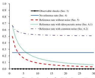
number of interbank transaction reports re‡ected in the reference rate. Figure 1 shows the relationship betweenV ar(is

t)andqfor the situations examined in Section 3,

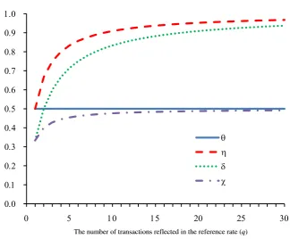
4, 5, 6.1, and 6.2, while Figure 2 shows the corresponding level of parameters of inference, such as , , , and . In the case of Section 3, where banks can distinguish between aggregate shocks and individual shocks,V ar(is

t)is equal to zero for all values ofq. In the case of Section 4, where banks

are unable to observe each shock separately, V ar(is

t) is not equal to zero. As shown in Figure 2,

the parameter of inference ( ) does not depend onq. Consequently,V ar(is

t)is positively constant

(0.25 in this benchmark example) for all values of q. In the case of Section 5, the reference rate exists and is noise-free. Whenqis extremely small, such asq= 1or 2,V ar(is

t)is larger than 0.25,

which is the corresponding value in Section 4. However, sinceV ar(is

t)is monotonically decreasing

withq,V ar(is

t)is less than 0.25 for su¢ciently large values ofq(speci…cally,q >4in this numerical

example), and converges to zero whenqapproaches in…nity. This illustrates the stabilizing e¤ects of the reference rate.

However, if the reference rate contains noisy components, the stabilizing e¤ects of the reference rate are signi…cantly reduced. In the case of Section 6.1 when the reference rate includes idiosyn-cratic noise,V ar(is

t)is larger than those in the case of Section 5, for a given value ofq. Nevertheless,

since the noise is idiosyncratic to individual transactions, the volatility of the market interest rate can be reduced by increasingq. However, in the case of common noise, which is examined in Section 6.2, V ar(is

t) does not converge to zero even ifq approaches in…nity. By increasing the value ofq,

the …rst term of (51) converges to 0.25. However, because of the presence of the third term of (51), V ar(is

t)is strictly larger than 0.25, which is the corresponding level in Section 4.

(16)

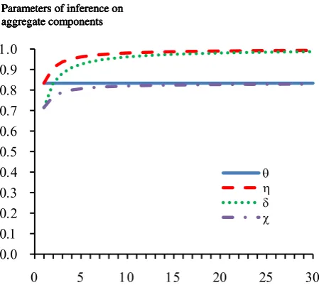
value ( 2 _{= 5}_:₀_{). For a given value of}_{q, the parameters of inference ( , , , and ) are larger than}

those in the benchmark example. Then, V ar(is

t)is lower than the benchmark value in the case of

Section 4. However, in the cases of Section 5, 6.1, and 6.2, V ar(is

t)is larger than the benchmark

value. This result can be understood as follows. In the presence of the reference rate, if 2 _{is large}

(compared to 2

"), banks set the inference parameter at a higher value, because banks know that the

reference rate contains more accurate information on the aggregate component. Higher inference parameters translate into higher …nal terms in (23), (39), and (51), thereby magnifying the volatility of the market interest rate. In the case of Section 4 where the reference rate is non-existent, this e¤ect is absent. Then the rise of 2 _{simply increases the inference parameter ( ), thereby lowering}

V ar(is t).

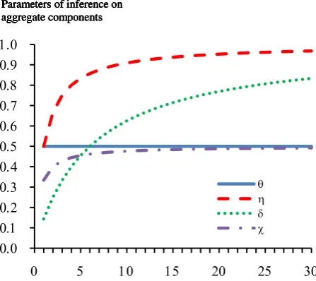
Panel (b) shows the case in which the variance of the idiosyncratic shock is larger than the benchmark value ( 2

"= 5:0). For a given value ofq, the parameters of inference ( , , , and ) are

smaller than those in the benchmark example. Then, V ar(is

t) is larger than the benchmark level

in all situations. In the case of Section 4, lower inference parameter ( ) leads to higherV ar(is t), as

shown in (14). This e¤ect also exists in other cases, as shown in the …rst terms of (23), (39), and (51). In addition, larger 2

"magni…esV ar(ist)by increasing the …nal terms in (23), (39), and (51).

As a result, for a given value ofq, larger 2

" leads to higherV ar(ist)in all situations.

Figure 4 presents a sensitivity analysis with respect to the variances of noise in the reported interest rates. Panel (a) shows the case in which the variance of idiosyncratic noise ( 2_{) is larger}

than the benchmark level. This rise in 2 _{simply lowers the parameter of inference in Section 6.1}

( ), for a given value of q. Then, V ar(is

t) is larger than in the benchmark example. Panel (b)

shows the case in which the variance of common noise is larger than the benchmark level. The rise in 2 _{simply lowers the parameter of inference in Section 6.2 ( ), for a given value of} _{q. Then,}

V ar(is

t)is larger than in the benchmark example. These results indicate that the market interest

rate becomes more volatile for large variances in either idiosyncratic noise or common noise.

8 Conclusion

(17)

cannot be reduced simply by increasing the number of sample transactions. This suggests that the noise in the interest rates reported by just a few of large banks can end up making the entire market more volatile, thereby lowering the correlation between the interbank interest rate and the central bank’s policy rate, and consequently impairing the transmission mechanism of monetary policy.

Appendix: When banks use !jt and !

q

t to infer the aggregate component

In Section 5, we have assumed that individual banks only use the information obtainable from the reference rate (!qt) to infer the aggregate component ( t). Here we assume that banks additionally

use the information on the fundamental shock in their individual transaction (!jt). This means that

the banks’ estimator of t takes the following form:

E_tj _t= ₁!j_t+ ₂!q_t: (A1)

Then, from (2), (4), (16), (17), and (A1), the parameters of ₁ and ₂are computed as follows:

1 =

2

(1 +q) 2₊ 2

"

; (A2)

2 =

q 2

(1 +q) 2₊ 2

"

: (A3)

By substituting (A1) into (5), the interest rate in thejth transaction is determined as follows:

ij_t=ip_t + (1 ₁)!j_t ₂!q_t: (A4)

The average interest rate across this sample of transactions is

iq_t = 1

q

X

k=1

ip_t+ (1 ₁)!k t 2!

q t =i

p

t+ (1 1 2)!

q

t: (A5)

Therefore, if the market-organizing institution provides the data ofiqt to individual banks, the

banks can obtain the value of!qt, from the simple calculation(i q t i

p

t)=(1 1 2) =!

q t.

From (2), (16), and (A4), the market interest rate is

im

t = _nlim_!1

1

n

X

j=1

ij_t= lim

n!1

1

n

X

j=1

h

ip_t+ (1 ₁)!j_t ₂!q_ti

= lim

n!1

1

n

X

j=1

h

ip_t+ (1 ₁)( _t+"_tj) ₂( _t+"q_t)i

= ipt+ (1 1 2) t 2"

q

(18)

ist=imt i p

t = (1 1 2) t 2"

q

t: (A7)

The variance of this spread is

V ar(is

t) = (1 1 2)2 2 + 22 2"=q: (A8)

In the limiting case ofq! 1_{, the volatility of the spread converges to zero:}

lim

q!1V ar(i

s

t) = lim q!1 1

(1 +q) 2

(1 +q) 2₊ 2

"

!2

2₊ q 2

(1 +q) 2 ₊ 2

"

!2 2

"=q= 0: (A9)

This result is the same as in Section 5.

References

[1] Abrantes-Metz, Rosa M., Michael Kraten, Albert D. Metz, and Gim S. Seow. (2012), “Libor Manipulation?”Journal of Banking & Finance, 36(1), pp. 136-150.

[2] Angelini, Paolo, Andrea Nobili, and Cristina Picillo. (2011), “The Interbank Market after August 2007: What Has Changed, and Why?”Journal of Money, Credit and Banking, 43(5), pp. 923-958.

[3] Ewerhart, Christian, Nuno Cassola, Steen Ejerskov, and Natacha Valla. (2007), “Manipulation in Money Markets”International Journal of Central Banking, 3(1), pp. 113-148.

[4] Freixas, Xavier, and Cornelia Holthausen. (2004), “Interbank Market Integration under Asym-metric Information”Review of Financial Studies, 18(2), pp. 459-490.

[5] Gefang, Deborah, Gary Koop, and Simon M. Potter. (2011), “Understanding Liquidity and Credit Risks in the Financial Crisis”Journal of Empirical Finance,18(5), pp. 903-914.

[6] Gyntelberg, Jacob and Philip Wooldridge. (2008), “Interbank Rate Fixings during the Recent Turmoil”BIS Quarterly Review, 2008 March, pp. 59-72.

(19)

[8] Kuo, Dennis, David Skeie, and James Vickery, “A Comparison of Libor to Other Measures of Bank Borrowing Costs,”mimeo.

[9] Lucas, Robert E. (1972), “Expectations and the Neutrality of Money,”Journal of Economic

Theory, 4(2), pp. 103-124.

[10] Lucas, Robert E. (1973), “Some International Evidence on Output-In‡ation Tradeo¤s,”

Amer-ican Economic Review, 63(3), pp. 326-334.

[11] Michaud, Francois-Louis, and Christian Upper. (2008), “What Drives Interbank Rates? Evi-dence from the Libor Panel,”BIS Quarterly Review, 2008 March, pp. 47-58.

[12] Morris, Stephen, and Hyun Song Shin. (2002), “Social Value of Public Information,”American

Economic Review, 92(5), pp. 1521-1534.

[13] Muto, Ichiro. (2013), “Productivity Growth, Transparency, and Monetary Policy,” Journal of

Economic Dynamics and Control, 37(1), pp. 329-344.

[14] Muto, Ichiro, Nao Sudo, and Shunichi Yoneyama (2012). “Productivity Slowdown in Japan’s Lost Decade: How Much of It is Atributed to Financial Factors?” mimeo.

[15] Phelps, Edmund. (1970), Microeconomic Foundations of Employment and In‡ation Theory, Norton, NY.

[16] Sudo, Nao. (2012), “Financial Markets, Monetary Policy and Reference Rates: Assessments in DSGE Framework” mimeo.

[17] Taylor, John B., and John C. Williams (2009), “A Black Swan in the Money Market,”American

Economic Journal: Macroeconomics, 1(1), pp. 58-83.

[18] Woodford, Michael. (2010), “Financial Intermediation and Macroeconomic Analysis,”Journal

(20)

0 7 0.8 0.9 1.0

Observable shocks (Sec. 3)

No reference rate (Sec. 4)

Reference rate without noise (Sec. 5) The volatility of the

interest rate spread (Var(is

t))

0.3 0.4 0.5 0.6 0.7 0.8 0.9 1.0

Reference rate without noise (Sec. 5)

Reference rate with idiosyncratic noise (Sec. 6.1)

Reference rate with common noise (Sec. 6.2) The volatility of the

t))

0.0 0.1 0.2 0.3 0.4 0.5 0.6 0.7 0.8 0.9 1.0

0 5 10 15 20 25 30

Reference rate with common noise (Sec. 6.2)

The number of transactions reflected in the reference rate (q) The volatility of the

t))

[image:20.595.127.445.173.432.2]

ote: The parameter values are set as: 

Figure 1: The volatility of the interest rate spread and the number of transactions reflected in the reference rate 0.0

0.1 0.2 0.3 0.4 0.5 0.6 0.7 0.8 0.9 1.0

0 5 10 15 20 25 30

(21)

  

Parameters of inference on aggregate components

        

 Parameters of inference on

aggregate components

          

      

   

The number of transactions reflected in the reference rate (q) Parameters of inference on

[image:21.595.130.455.178.446.2]

ote: The parameter values are set as: 

Figure 2: Parameters of inference and the number of transactions reflected in the reference rate 

         

      

   

(22)

0 9 1.0

The volatility of the interest rate spread (Var(is_t))



Parameters of inference on aggregate components 0.3 0.4 0.5 0.6 0.7 0.8 0.9 1.0

           Parameters of inference on

aggregate components 0.0 0.1 0.2 0.3 0.4 0.5 0.6 0.7 0.8 0.9 1.0

0 5 10 15 20 25 30

interest rate spread (Var(is_t))

                     

(a) 

0.0 0.1 0.2 0.3 0.4 0.5 0.6 0.7 0.8 0.9 1.0

0 5 10 15 20 25 30

0 9 1.0

                     



Parameters of inference on aggregate components 0.0 0.1 0.2 0.3 0.4 0.5 0.6 0.7 0.8 0.9 1.0

0 5 10 15 20 25 30

0.3 0.4 0.5 0.6 0.7 0.8 0.9 1.0

                     

aggregate components        

0 5 10 15 20 25 30

0.0 0.1 0.2 0.3 0.4 0.5 0.6 0.7 0.8 0.9 1.0

0 5 10 15 20 25 30

                     

aggregate components                  

[image:22.595.305.530.107.311.2]

(23)

0 9 1.0



Parameters of inference on aggregate components 0.3 0.4 0.5 0.6 0.7 0.8 0.9 1.0

Observable shocks (Sec. 3) No reference rate (Sec. 4) Reference rate without noise (Sec. 5)

Reference rate with idiosyncratic noise (Sec. 6.1) Reference rate with common noise (Sec. 6.2)

        

0 5 10 15 20 25 30

                     

(a) 

0.0 0.1 0.2 0.3 0.4 0.5 0.6 0.7 0.8 0.9 1.0

0 5 10 15 20 25 30

0 9 1.0

                     



0 5 10 15 20 25 30

0.3 0.4 0.5 0.6 0.7 0.8 0.9 1.0

                     

aggregate components        

0 5 10 15 20 25 30

0.0 0.1 0.2 0.3 0.4 0.5 0.6 0.7 0.8 0.9 1.0

0 5 10 15 20 25 30

                     

aggregate components                  

[image:23.595.305.529.110.309.2]