A model of technological progress in the microprocessor industry

Munich Personal RePEc Archive

A model of technological progress in the

microprocessor industry

Pillai, Unni

University at Albany, SUNY

27 June 2011

A Model of Technological Progress in the

Microprocessor Industry.

Unni Pillai

∗_{Pillai: University at Albany - SUNY, 255 Fuller Road, Albany, NY 12203, [email protected]. I am}

Abstract

This paper develops a model of technological progress in the microprocessor industry

that connects the seemingly disparate engineering and economic measures of technological

progress. Technological progress in the microprocessor industry is driven by the repeated

adoption of higher quality vintages of capital equipment produced by the upstream

semicon-ductor equipment industry. The model characterizes the optimal adoption decision of a

micro-processor firm and the resulting rate of technological progress. In conjunction with parameters

estimated using a new dataset of the microprocessor industry, the model suggests explanations

for the acceleration in technological progress during 1990-2000 and the subsequent slowdown.

(JEL: O31, L63)

1

Introduction

A number of studies seeking to explain the increase in productivity growth in the US economy

during the second half of 1990s credit a central role to an acceleration in technological progress in the microprocessor industry.1 _{The cause of the acceleration has been debated in many}

aca-demic, industrial and policy forums.2 _{The rate of technological progress in the microprocessor}

industry slowed down after 2000. There has been no convincing explanation of the acceleration

or slowdown to date. Jorgenson (2001) points to the need for an economic model of technological progress in this industry to understand the cause of the acceleration. The multifaceted nature of

technological progress in microprocessors has generated a plethora of characterizations of techno-logical progress in this industry. Engineers favor a description based on Moore’s law - a statement

made in Moore (1975) that the number of transistors on a semiconductor chip doubles every two

1_{Jorgenson (2001) was the first to point out the importance of microprocessor industry. See also Oliner and Sichel}

(2002a) and Gordon (2002).

2 _{See for example the proceedings of the workshop on Measuring and Sustaining the New Economy (2002),}

years.3 _{Scientists prefer the rate at which the physical dimensions of an individual transistor has}

gone down, which has decreased by a factor of roughly 0.7 every 2-3 years. Business analysts in the semiconductor industry resort to the rate at which the processing speed (also called

perfor-mance) of microprocessors have increased, while economists use the rate at which price per quality unit of microprocessors have declined.4 _{By incorporating choices over engineering variables like}

transistor size and number of transistors, alongside economic variables like price, quantity and time of new technology adoption, the model in this paper successfully connects these disparate

engineering and economic measures of technological progress.

The model also formalizes the commonly held notion in the industry that the key decision

fac-ing a microprocessor firm is when to adopt a new vintage of capital equipment. Once the adoption decision has been made, profit maximizing considerations dictate a clear choice of the size of

tran-sistor to use, the number of trantran-sistors to use, the processing speed and the price per quality unit. A contribution of this paper is the characterization of the adoption decision and the resulting time

paths for the four variables. The optimal time to adopt new capital equipment is when the lag be-hind the best available capital equipment reaches a threshold value. This result has been previously

obtained in other models of technology adoption, including Balcer and Lippman (1984), Dixit and Pindyck (1994), Doraszelski (2001), and Farzin, Huisman and Kort (1998).5 _{The predictions of}

the model regarding the adoption policy and the time paths of the four measures of technological progress fit well with the empirical observations, which are outlined in section 2. The

impor-3_{A transistor is the basic electronic component in a microprocessor. See section 2 for more details. Moore (1965)}

predicted the number of transistors on a chip to double every year, which was later revised to doubling every two years in Moore (1975).

4_{Table 3 gives average growth rates for performance and price per quality unit.}

5_{Although not directly related, this paper is in the spirit of Griliches (1957), who uses a model of technology}

tance of the adoption of new capital equipment highlights the fact that technological progress in

microprocessors is driven to a large extent by innovations in the upstream semiconductor equip-ment industry.6 _{Semiconductor equipment firms like Nikon, Canon, Applied Materials and ASML}

invent new generations of capital equipment which allow microprocessor firms like INTEL and AMD to fabricate smaller transistors, enabling them to make higher performance microprocessors.

The notion that the repeated adoption of higher quality vintages of capital equipment is the driver of technological progress in the microprocessor industry has been emphasized in Aizcorbe and

Kortum (2005).

A distinguishing feature of this paper is that it models technology in the industry in more detail

than is common in economic models. This more detailed incorporation of the technology turns out to be essential to understand the causes of the acceleration and slowdown in technological

progress, because it helps to separate out the contribution of the semiconductor equipment firms from that of microprocessor firms towards technological progress in the microprocessor industry.

There have been many previous studies of the acceleration and slowdown, including Jorgenson (2001), Aizcorbe (2005), Aizcorbe, Oliner and Sichel (2006) and Flamm (2004). The studies above

characterize the rate of technological progress in terms of the rate at which price per quality unit has declined for microprocessors.7 _{This approach however has the limitation, as noted in Aizcorbe et}

al. (2006), that changes in prices brought about by changes in demand and competitive conditions can be mistakenly attributed to changes in the rate of technological progress. To overcome this

problem, I use the notion of technological progress as the growth of microprocessor performance.8

Performance, or processing speed, is a measure of how fast a microprocessor can execute software

programs. Nordhaus (2001) gives a detailed description of the use of performance as a measure of technological progress in computing, and compares it with the hedonic price based approach.

6_{Section 2 elaborates on this link between technological progress in the microprocessor industry and the adoption}

of new vintages of capital equipment.

7_{The price per quality unit is estimated using hedonic regressions.}

8_{Performance is the commonly used measure for comparing microprocessors in computer science. It is the}

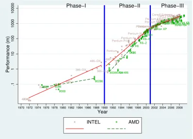
Figure 1 shows the performance of microprocessors produced by two main microprocessor

companies, INTEL and AMD, during 1971-2008. As the figure shows, growth rate of performance increased during 1990-2000 and decreased subsequently. Table 3 shows the magnitude of the

increase in growth rate of performance and compares it with the growth rate of price per quality unit declines mentioned in Aizcorbe et al. (2006). As can be seen from Table 3, the growth of

performance closely follows the hedonic price based measure of technological progress.

40048008 8085

286 386−DX

486−DX

386−SL 486−SL

Pentium

Pentium ProPentium II Pentium III

Pentium 4Pentium 4−M

Pentium MPentium EEPentium DCore Duo Core 2 Extreme_{Core 2 Quad}

Core 2 Duo Core 2 Solo

8080 8086 8088

80286

80386−DXAm 486 5X86K5

K6 K6−2

K6−III Athlon

Athlon XP Athlon 64 Athlon FXAthlon 64 X2_{Turion 64 X2}

Turion 64

Phase−I Phase−II Phase−III

.1

1

10

100

1000

10000

Performance (m)

1970 1972 1974 1976 1978 1980 1982 1984 1986 1988 1990 1992 1994 1996 1998 2000 2002 2004 2006 2008

Year

INTEL AMD

Figure 1: The Acceleration and Slowdown for INTEL and AMD.

The model in this paper implies that in steady state, the mean growth rate of performance is

section 3.3 for a description of efficiency in this industry). The model, together with empirical

es-timates of the parameters, imply that the acceleration during 1990-2000 was caused by an increase in the innovation rate in the upstream semiconductor equipment industry, while the slowdown

af-ter 2000 was caused by a decrease in the efficiency with which the microprocessor industry used the upstream innovations. In a nutshell, the upstream semiconductor equipment firms were

re-sponsible for the acceleration and the downstream microprocessor firms for the slowdown. These explanations also find support in previous papers. Jorgenson (2001) suggests that the acceleration

was caused by a decrease in the technology cycle in the semiconductor equipment industry from 3 yrs to 2 yrs, a fact confirmed in Figure 2. An increase in the innovation rate in the semiconductor

equipment industry leads to a decrease in the technology cycle, as shown in section 5 in this paper. Aizcorbe et al. (2006) also find support for the explanation in Jorgenson (2001), but they remain

cautious about this explanation because the innovation rate did not drop during the period of the slowdown. This paper provides the missing link in the explanation. Even though the innovation

rate in the semiconductor equipment industry did not drop, there was a drop in the efficiency with which microprocessor firms used these innovations during the slowdown period.

The slowdown since 2000 has reduced the contribution of the microprocessor industry to ag-gregate productivity growth. The impact of the acceleration and slowdown on total factor

produc-tivity (TFP) growth in the US economy can be calculated using the method suggested in Oliner and Sichel (2002a). In their method, the aggregate TFP growth is the weighted average of the TFP

growth in the different sectors in the economy, where the weight for each sector is its gross output as a share of the aggregate output.9 _{Using the growth rate of performance as a proxy for the TFP}

growth rate in the microprocessor industry, Table 5 shows that the contribution of microproces-sor industry to aggregate TFP growth quadrupled during the acceleration and more than halved

during the slowdown. This paper suggests that technological progress in the microprocessor

in-9_{The theoretical justification for the method is given in Hulten (1978). Note that this method captures only the}

dustry is unlikely to return to the accelerated path during 1990-2000, unless the industry finds a

way to increase the efficiency with which it is using the innovations generated by the semiconduc-tor equipment industry. I now turn to a brief description of the connection between technological

progress in the microprocessor industry and innovations in the upstream semiconductor equipment industry.

2

Technological Progress in the Microprocessor Industry - the

link to the Semiconductor Equipment Industry

A microprocessor can be thought of as a collection of transistors which operate in tandem to

exe-cute instructions contained in different software programs. The performance of a microprocessor can be increased either by increasing the speed of operation of each individual transistor or by

using more transistors so that more software instructions can be executed simultaneously (in par-allel). The speed of operation of each individual transistor is limited by its size, smaller transistors

are faster. The size of each transistor is in turn limited by the quality of the capital equipment used in manufacturing the microprocessor. Innovations in the semiconductor equipment industry lead to

capital equipment that can make smaller transistors.10 _{The evolution of the microprocessor}

indus-try towards faster microprocessors traces the repeated adoption of higher quality vintages of capital

equipment produced by the semiconductor equipment firms, each vintage of capital equipment be-ing marked by the size (or length) of the transistor that the equipment allows the microprocessor

industry to make. Since these transistor sizes are really small, they are usually quoted in microns (µ), which is a millionth of a meter. The leading microprocessor firm, INTEL, has adopted

four-10_{The equipment industry has a separate classification under the North American Industrial Classification System}

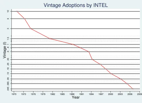
teen such vintages during 1971-2008, 10µ, 6µ, 3µ, 1.5µ, 1µ, 0.8µ, 0.6µ, 0.35µ, 0.25µ, 0.18µ, 0.13µ, 0.09µ, 0.065µand 0.045µ. Figure 2 plots the different vintages of semiconductor capital equipment that INTEL and AMD have adopted against the date of adoption. In the progression

Contact Aligner Proximity Aligner Projection Aligner G−Line Stepper G−Line Stepper G−Line Stepper

Advanced G−Line Stepper Advanced G−Line Stepper

I−Line Stepper I−Line 436 nm I−Line 436 nm I−Line 436 nm I−Line 436 nm

I−Line 365 nm DUV DUV

Advanced DUV DUV 248 nm DUV 248 nm

DUV 193 nm DUV 193 nm DUV 193 nm DUV 193 nm DUV 193 nm

Phase Shift Mask Phase Shift Mask Phase Shift Mask Phase Shift Mask Phase Shift Mask Phase Shift Mask Phase Shift Mask Phase Shift Mask

Double Patterning

Phase−I Phase−II Phase−III

.045 .065 .09 .13 .18 .25 .35 .5 .6 .7 .8 1 1.5 3 6 10 Vintage (l)

71 74 76 82 89 91 94 95 98 99 01 04 05 07

Date of Adoption

INTEL AMD

Adoption of Vintages of Semiconductor Equipment

Figure 2: INTEL and AMD’s adoption of new vintages of semiconductor capital equipment.

Notes:The date of adoption of a vintage is taken to be the date on which INTEL (or AMD) released the first

microprocessor manufactured with that vintage. The dates marked on the x-axis are Intel’s adoption dates. Note the decrease in the average time interval between adoptions after Phase I. This is the reduction in technology cycle that has been noted in Jorgenson (2001), Aizcorbe et al. (2006) and Flamm (2004).

through these fourteen vintages from 1971 to 2008, the transistor size has decreased by a factor

of size ℓ. A lower ℓ thus implies a higher quality vintage. Equipped with this brief introduction to technology in the microprocessor industry, I document below four stylized facts about the evo-lution of the four measures of technological progress in the microprocessor industry mentioned in

the introduction. I denote the time period 1971-1989 as Phase I, the period 1990-2000 as Phase II and the period 2001-2008 as Phase III.11 _{The four stylized facts are:}

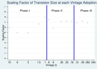
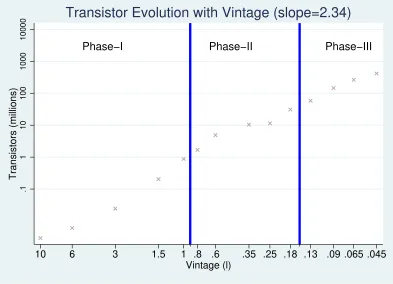
1. The adoption of each new vintage of capital equipment decreases the transistor size ℓ by roughly the same factor (see Figure 4). For brevity, I will call this as thescaling factor.

2. The number of transistors in a microprocessor, T, increases at roughly double the rate at which transistor sizeℓdecreases (see Figure 5).

3. Performance grows at a roughly constant rate within each phase. The average growth rate of performance almost doubled going from Phase I to Phase II (the acceleration) and more

than halved going from Phase II to Phase III (the slowdown). (See Figure 1 and Table 3.)

4. Price/Performance (price per quality unit) declines at a roughly constant rate within each

phase. The average decline rate of price/performance increased going from Phase I to Phase II (the acceleration) and decreased going from Phase II to Phase III (the slowdown). (See

Table 3.)

The next section develops a model that is consistent with the pattern of evolution of the four measures of technological progress documented in the stylized facts above.

3

The Model

The model is in continuous time. I develop the model in a few stages starting with the

semicon-ductor equipment industry.

11_{This section, and the other empirical sections of this paper, uses a new dataset of the microprocessor industry that}

3.1

The Semiconductor Equipment Industry

Although the semiconductor equipment industry consists of a large number of firms which manu-facture different types machinery, from the point of view of technological progress in the

micropro-cessor industry the most important function that these companies serve is that they undertake the R&D necessary to manufacture the next vintage of capital equipment. Hence I lump all these

com-panies together as the semiconductor equipment industry. I denote the frontier or highest quality vintage (i.e. the vintage with the smallest transistor size) by ℓ¯. The R&D done by the semicon-ductor equipment industry generates innovations that follow a Poisson process with parameterλ. Each innovation reducesℓ¯by a fixed factorδ, whereδ <1. Hence the stochastic process forℓ¯can be written as

¯

ℓ(t) =δN(t)ℓ¯(0),

N(t)is a P oisson process with rate λ.

I now turn to a description of the demand side of the model.

3.2

Demand in the Microprocessor Industry

Consumers care only about the performance of microprocessors. I assume a stationary inverse demand curve, given by,

p(t)

m(t) =D{m(t)y(t)}

−1

η . (1)

Here p(t)is the price of microprocessor sold at time t, m(t) is the performance (quality) of the microprocessor andy(t)is the number of microprocessors demanded. The price per quality unit is

p(t)

m(t), andm(t)y(t)is the total number of quality units demanded. The basic assumption behind

the demand structure is that total quality units demanded has a constant elasticity, η, in price per quality unit. One obvious abstraction in this demand specification is the absence of dynamic

making process by consumers could have been a cause of the acceleration and slowdown, so I

ignore this aspect of demand.12 _{I now describe the technology side of the model.}

3.3

Technology in the Microprocessor Industry

A microprocessor firm like INTEL chooses the quality (performance) of its product to maximize profits. The common way to model the quality choice of a firm is to have the firm pay a fixed

cost to obtain an improvement in quality (e.g. in Sutton (2001).13_{. The production process in the}

microprocessor industry, however, gives rise to a peculiar tradeoff between performance and costs

not captured in such models. Equations (2) and (3) below, which capture the central aspects of production technology in the microprocessor industry, illustrate this tradeoff. A firm in the

micro-processor industry has two ways to increase the performance of its micromicro-processor. First, it can adopt a new vintage of capital equipment which enables it to fabricate smaller (lowerℓ) and hence faster transistors.14 _{Second, it can increase the number of transistors that it uses in its}

microproces-sor, which allows the firm to fabricate more units working in parallel in the microprocesmicroproces-sor, thus

increasing performance. Performance can thus be written as a function of the number of transistors

T and the vintage of capital equipmentℓ,

m(T, ℓ) = T α

ℓ . (2)

12 _{See Gordon (2009) for a model of dynamic decision making and replacement cycles in the microprocessor}

industry.

13_{In other models, like Pakes and McGuire (1994), paying the fixed cost increases the probability of making an}

improvement in quality.

14_{Reducingℓby a given factor increases the speed of each transistor by the same factor (see Ronen, Mendelson, Lai,}

A microprocessor firm has the choice of increasing performance by increasing the number of

tran-sistors, without having to reduce ℓ by adopting a new vintage of capital equipment. Such an approach, however, increases the marginal cost of producing a microprocessor because it increases

the fraction of microprocessors that are defective in any lot, a feature stemming from the peculiar-ities of the semiconductor production process. In any given lot of microprocessors manufactured,

a certain fraction would be defective because of manufacturing imperfections arising from con-tamination by dust particles in the course of production. The fraction of defective microprocessors

increases with the physical area A of the microprocessor because larger microprocessors have a higher probability of being contaminated by dust particles. A commonly used yieldmodel in the

industry gives the fraction of good microprocessors in any given lot ase−A_{, whereAis the area of}

the microprocessor.15 _{Hence, ifc¯is the unit cost of producing a raw microprocessor, the marginal}

cost of producing a good microprocessor is¯ceA_{. Since the area of each individual transistor isℓ}2_,

the area the microprocessor containingT transistors isA =T ℓ2_{. Substituting forA, the marginal}

cost is given by,

c(T, ℓ) = ¯ceT ℓ2 (3)

Increasing T without reducing ℓ rapidly escalates the marginal cost. If the firm reduces ℓ by adopting a new vintage and increasesT in proportion to 1

ℓ2, then the marginal cost remains constant

while performance increases. This is indeed the policy that the model in this paper predicts to be the

optimal policy, as well the policy that microprocessor firms have followed in practice (see stylized fact 2 and Figure 5). Although adopting a new vintage allows a microprocessor firm to keep

marginal cost constant while increasing performance, the firm has to expend a considerable amount

15_{The formula for the fraction good microprocessors (yield) used in this paper, e}−A

, is called the Poisson yield equation. The Poisson yield is usually given ase−σS

of engineering effort in perfecting the production process with the new vintage of machines.16 _I

capture this fixed cost with the functionF(ℓ), which increases asℓdecreases. The fixed costF(ℓ)

does not include the user cost of capital, which is incorporated into the unit cost of producing a

raw microprocessor,¯c.

The functions m(T, ℓ), c(T, ℓ) andF(ℓ)capture the technology in this industry. Note that in the function m(T, ℓ) in equation (2), the ability of a microprocessor firm to translate increases in T to increases inm depends on the parameter α. The parameter α is a measure of quality of design used in the microprocessor. With a superior design (higher α), a microprocessor firm can get bigger performance increments from a given increase in the number of transistors. This design

quality is thus a measure of the technicalefficiencyof the microprocessor firm. In section 5, I argue that a drop in efficiency αcaused the slowdown in technological progress in the industry. Using the primitives of demand and technology in sections (3.2) and (3.3), the next section lays down the profit maximization problem faced by a microprocessor firm.

3.4

The Profit Maximization Problem of the Microprocessor Firm

Before turning to formal description of the microprocessor firm’s problem, I make two

assump-tions. First, I assume that the market for microprocessors consists of a single firm facing the demand curve in equation (1). Although there are two major microprocessor producers, INTEL

and AMD, INTEL has been at the forefront of making innovations in the industry while AMD has usually lagged behind. INTEL has also occupied 75%-90% of the microprocessor market during

the time period considered in this paper. Moreover, in a paper exploring whether AMD spurs IN-TEL to innovate, Goettler and Gordon (2009) find that innovation is more in an ININ-TEL monopoly

than in an INTEL-AMD duopoly. In the light of these arguments, modeling the industry as a duopoly would complicate the analysis while providing little help in finding explanations of the

acceleration and slowdown. Second, I assume that the microprocessor firm sells only the highest

16_{INTEL has estimated the cost of adoption next vintage of capital equipment (0.032µ) to be 7 billions dollars. See}

quality (performance) microprocessor. As soon as a better product is made, the entire production

is moved to the new product. This assumption helps focus on the factors that determine the rate at which microprocessor performance is growing.

Given the Poisson arrival rateλof innovations to capital equipment, each of which reduceℓ¯by a factorδ, the microprocessor firm has to choose the time paths of performance, marginal cost, the number of microprocessors to produce, the vintage of capital equipment to use, and the sequence of times at which to adopt new vintages of capital equipment,{τj}∞_j=0. The choice of performance

and marginal cost can equivalently be stated in terms of choice of number of transistors and vintage of capital equipment. Formally, the problem of the microprocessor firm is,17

max

E



 ∞ Z

0

e−ρt[p(t)−c(T, ℓ)]y(t)dt −

∞ X

j=0

e−ρτj_F(ℓ(τ

j))





T(t),ℓ(t),y(t),{τj}∞j=0

subject to p(t)

m(T, ℓ) =D{m(T, ℓ)y(t)}

−1

η _,

m(T, ℓ) = T α

ℓ , c(T, ℓ) = ¯ceT ℓ

2

ℓ(t)≥ℓ¯(t), ℓ¯(0) given,

¯

ℓ(t) = δN(t)ℓ¯(0), N(t)is a P oisson process with rate λ.

The term in the outer square brackets is the present discounted value of net profits, which is the difference between the present discounted values of gross profits (the integral term in the objective

function) and the sum of fixed cost of adopting new vintages (the summation term in the objective function). The first constraint is the demand curve in equation (1), the second and third are the

technology constraints in equations (2) and (3), the fourth simply states that the firm can at best

17_{To avoid notational clutter, I have abbreviatedm(T(t), ℓ(t))asm(T, ℓ)andc(T(t), ℓ(t))asC(T, ℓ)in the}

be using the best vintage currently available, and the last specifies the stochastic process for the

evolution of the best (frontier) vintage. I restrictη >1to make the firm’s problem well defined.

3.5

Microprocessor Firm’s Optimal Policies

The optimal choice ofT andydepend only on the current value ofℓ. Hence I solve the problem by first solving the static problem of choosingT andyfor a givenℓand then embedding this solution back into the problem, to solve the dynamic problem of choosing the optimal times {τj}∞_j=0 at

which to adopt newℓ. Substituting the constraints into the objective function, it can be seen that the solution to the static problem is as follows. Along an optimal path ofT andy, the following condition has to hold,

T∗(ℓ) =α1

ℓ2. (4)

Substituting equation (4) into equation (3) gives marginal cost as

c∗(ℓ) = ¯ceα ≡c∗. (5)

The firm’s optimal policy is thus to choose T in proportion to 1

ℓ2 and hence keep the marginal

cost at c∗ = ¯ceα_{, irrespective of the vintage ℓ used. The optimality conditions in equations (4)}

and (5) result from the tradeoff between performance and marginal cost explained in section 3.3.

Substituting equation (4) into equation (2) gives the optimal performance as,

m∗(ℓ) = T

∗_(ℓ)α

ℓ =α

α 1

ℓ1+2α. (6)

i.e. performance grows at1 + 2αtimes the rate at whichℓdecreases. The term1 + 2αshows the twin benefits that a microprocessor firm gets from using a vintage with a smallerℓ. The exponent

2α represents the indirect benefit of smaller ℓ on m through T, and the exponent 1 represents the direct benefit arising from the fact that smaller transistors are faster. The optimal number of microprocessors to producey∗_(ℓ)is,

y∗(ℓ) = (η−1) 1 ¯

ceα

π

whereπandϕare given by,

π =

µ

(η−1)α α

¯

ceα

¶η−1µ

D η

¶η

, (8)

ϕ = (1 + 2α)(η−1). (9)

Substituting the solutions formandyinto the demand equation (1) gives the optimal price as,

p∗(ℓ) = η

η−1[¯ce α

]≡p∗, (10)

i.e. the price of a microprocessor is a constant markup over the marginal cost of production, the term inside square brackets being the marginal cost of production. The solutionsp∗ andy∗(ℓ)give the revenue along the optimal path as

r∗(ℓ) =ηπ

ℓϕ. (11)

As expected for a constant elasticity demand curve, the gross profit is a constant fraction _η1 of revenue, and is given by

π∗(ℓ) = π

ℓϕ. (12)

Using the gross profit function in equation (12), the microprocessor firm’s problem can be rewritten as max E   ∞ Z 0

e−ρtπ∗(ℓ(t))dt −

∞ X

j=0

e−ρτj_F(ℓ(τ

j))





ℓ(t),{τj}∞j=0

subject to π∗_{(ℓ(t)) =} π

ℓ(t)ϕ,

ℓ(t)≥ℓ¯(t), ℓ¯(t) = δN(t)ℓ¯(0), N(t)is a P oisson process with rate λ.

I solve the problem using dynamic programming. The dynamic programming problem is most conveniently expressed by choosing the state variables asℓ¯, the frontier vintage, andx= ℓ¯

ℓ, which

arriving in a small interval of time∆tisλ∆t, and the probability of more than one innovation is approximately zero. Hence the value function should satisfy the Bellman equation,

V(¯ℓ, x) = _µ¯π

ℓ x

¶ϕ∆t + e −ρ∆t£

(1−λ∆t)V(¯ℓ, x)

+ λ∆t M ax©

V(δ¯l, δx), V(δℓ,¯1)−F(δℓ¯)ª

].

The first term on the right hand side is the profit that the firm receives in a small interval of time

∆t, the second term is the discounted expected payoff after ∆t. With probability 1−λ∆t no innovations arrive in which case the firm’s value remains at V(¯ℓ, x). With probability λ∆t one innovation arrives, in which case the firm has to choose between not adopting this innovation and getting valueV(δℓ, δx¯ )or adopting it and getting a valueV(δℓ,¯1)−F(δℓ¯).

I assume that F(ℓ) is homogeneous of degree −ϕ, the same degree of homogeneity as the gross profit function, π∗(ℓ). If this were not true, then one would get a non-stationary model. If

F(ℓ)was increasing at a faster rate inℓthanπ∗(ℓ), then the factor by whichℓscales at each adop-tion (the scaling factor) would decrease over time, getting closer to 0. If Ifπ∗(ℓ)was increasing at a faster rate than F(ℓ), then the scaling factor would increase over time, getting closer to 1. However, as Figure 4 shows, the scaling factor does not show any systematic variation over time,

consistent with the assumption thatF(ℓ)is homogeneous of degree−ϕ. The assumption thatF(ℓ)

is homogeneous of degree−ϕ implies thatV(¯ℓ, x)is homogenous of degree −ϕin ℓ¯, and hence

V(¯l, x) = ¯l−ϕ_{V(1, x) = ¯ℓ}−ϕ_{v(x) , where V(1, x) = v(x). The dynamic program can thus be}

expressed with a single state variable,x. Re-writing with the single state variable, and taking the limit∆t→0, the Bellman equation simplifies to,

ρv(x) =xϕπ+λ

·

1

δϕM ax{v(δx), v(1)−F(1)} −v(x)

¸

. (13)

The left hand side of the equation is the payoff to owning the firm, which is the sum of the instan-taneous payoff and the change in value which occurs if an innovation arrives, an event with hazard

lag behind the frontierx, reaches a threshold valuesx∗_{(see Proposition 1 for proof). The threshold}

valuex∗satisfies the following equation,

ρ(v(1)−F(1)) =πx∗ϕ+λ

½

1

δϕ[v(1)−F(1)]−[v(1)−F(1)]

¾

. (14)

Equation (14) is the value matching condition mentioned in Dixit and Pindyck (1994) and Farzin

et al. (1998). The firm adopts at the point where the value to adopting is equal to the value to waiting. The value to adopting immediately is the left hand side of the equation, the firms jumps

to the frontier but it has to pay the fixed cost F(1). The term on the right hand side is the value to waiting which is the sum of the instantaneous payoff and the change in value that occurs if an

innovation arrives at that moment in time. Equation (14) can be rewritten to give the threshold valuex∗_as,

x∗ =

½µ

ρ+λ− λ

δϕ

¶ µ

v(1)−F(1)

π

¶¾_ϕ1

. (15)

Equation (15) requiresρ > λ( 1

δϕ −1).

18 _{Since each innovation shrinksℓ}¯_{byδ, this implies that it}

is optimal to adopt at everyn∗th innovation, wheren∗is the smallest integer such thatδn∗ ≤x∗. It is easy to summarize the dynamic policy using the simple diagram below. The possible values of

0 _δn∗ ... δ2 δ 1

x

xare1, δ, δ2, ..., δn∗−1. Starting fromx= 1, the value ofxdecreases toδ,δ2,.., as the equipment sector produces its stream of innovations. When then∗_{th innovation arrives, the firm adopts it and}

xbecomes equal to one again. This cycle repeats.

I summarize the results above. The microprocessor firm adopts everyn∗_{th innovation made by}

the semiconductor equipment industry and henceℓused by the firm scales repeatedly by the same

18_{If discount factorρis not high enough, then discounted net profits are increasing over time and there will be no}

factorδn∗. Asℓdecreases, the firm chooses to increase transistor count (T) and performance (m) in proportion to 1

ℓ2 and

1

ℓ(1+2α) respectively. The firm chooses to maintain the marginal cost at

c∗_{and charge a pricep}∗ _{per microprocessor, while increasing the number of units produced (y) in}

proportion to _ℓ1ϕ, whereϕ = (1+2α)(η−1). Revenue and gross profits also increase in proportion

to _ℓ1ϕ. This concludes the development of model.

4

Discussion

In this section I show that the model’s predictions are consistent with the stylized facts documented in section 2 and use the model to connect the four measures of technological progress mentioned in

the introduction. The optimal choices of the firm with regard to engineering variables like number of transistors and performance as well as economic variables like quantity, profits and revenue are

determined by the vintageℓof capital equipment that the firm is using, and evolves with the change in ℓ at each new vintage adoption. The model thus formalizes the commonly held notion in the microprocessor industry that the adoption of new vintages of capital equipment is the key driving force in the industry.

The model predicts that at the adoption of each new vintage, the transistor sizeℓshould scale by the same factorδn∗, accounting for stylized fact 1. As equation (4) shows, the model predicts that the firm’s optimal policy is to increaseT in proportion to 1

ℓ2, accounting for stylized fact 2. I

show below that the mean growth rate ofmis given by

gm =−(1 + 2α)λln(δ). (16)

Thus the mean growth rate of m is constant as long as α and λ does not change. I argue in section 5 that changes in gm between the three phases were caused by shifts inλ andα. Within

one more testable prediction, that the microprocessor firm should adopt only occasionally, and

should skip some innovations. In Figure 3, I plot the vintages adopted by INTEL (solid horizontal lines). The dotted lines are some of the vintages for which capital equipment was sold by some of

the leading semiconductor equipment producers, but were not used by INTEL.19 _{As can be seen}

from the graph, there were quite a number of vintages which INTEL did not adopt, in line with the

prediction of the model.

The model connects the four measures of technological progress mentioned in the introduction.

Since the firm’s policy is to adopt everyn∗th innovation, the mean growth rate ofℓ will be deter-mined by the stochastic process generating the innovations. Since the innovations follow a Poisson

process with rate λ and stepsize δ, the mean growth rate of ℓ is given by gℓ = λln(δ).20 From

equation (4) it is clear thatT increases at twice the rate at whichℓdecreases, i.e. gT =−2λln(δ).

From equation (6) it follows that gm = −(1 + 2α)gℓ. This gives the mean growth rate of

m as, gm = −(1 + 2α)λln(δ). Finally, since the price of a microprocessor remains constant

over time, the price per performance decreases at the rate at which performance increases, i.e.

gpm = (1 + 2α)λlnδ. The four expressions above bring out the relationships between the four

measures of technological progress in the industry. While the rate of reduction in transistor size (gℓ)

and growth in number of transistors per microprocessor (gT) is fixed by the innovation parameters

λandδin the upstream semiconductor equipment industry, the rate of growth of performance (gm)

and price/perperformance (gpm) depend also on the the efficiencyαwith which the microprocessor

firm uses the upstream innovations.

19_{The vintages for the dotted lines were produced by one of the following equipment companies - ASML, Nikon,}

GCA, SVGL, Parkin-Elmer and Ultratech.

20_{Note thatg}

.045

.065

.09

.13

.18

.25

.35

.6

.8

1

1.5

3

6

10

Vintage (l)

1970 1973 1976 1979 1982 1985 1988 1991 1994 1997 2000 2003 2006 2009

Year

Vintage Adoptions by INTEL

Figure 3: INTEL does not adopt all vintages.

Notes:The solid lines are vintages that were adopted by INTEL. The dotted lines are vintages that were produced by

5

Explanations for the Acceleration and Slowdown

In this section I use the model to study the acceleration and subsequent slowdown in

technolog-ical progress, measured as growth of performance. I will argue below that the acceleration was caused by an unanticipated increase in the upstream innovation rate λ, and the slowdown by an unanticipated decrease in the efficiency α with which INTEL used upstream innovations. These explanations are consistent with the model, since it can be seen from equation (16) that an increase

inλincreasesgm and a decrease inαdecreasesgm. I explore below whether the model’s

predic-tions about the response of other variables to unanticipated changes inλandαare consistent with the data.

The changes inλdo not affect the static policies -T∗(ℓ),m∗(ℓ),y∗(ℓ),c∗ orp∗, as can be seen from equations (4)-(10). Such changes do affect the threshold lagx∗in equation (15) and possibly the optimal adoption policy,n∗. To characterize the changes inn∗ induced by changes inλ, I use the fact that any change inn∗ would affect the present discounted value of the firm. Let V¯(n, λ)

be the present discounted value of the firm if it adopts everynth innovation, given an arrival rate

λ. Clearly, the optimal adoption policyn∗ should satisfy

n∗ = arg max n

¯

V(n, λ).

As shown in Proposition 3,

¯

V(n, λ) = _¯1

ℓϕ₀



 

n

1−³_ρ+λ _λ´noπ_ρ −³_δ1ϕ_ρ λ +λ

´n

F(1) 1−³ 1

δϕρ+λλ

´n



 .

I evaluate the expression V¯(n, λ) for plausible parameter values of {δ, F(1), π, ρ, ϕ,ℓ¯0} for

dif-ferent values ofλand n. Figure 6 shows the result of a sample simulation for n = {3,4,5}. As can be seen from the figure,n∗ _{is weakly increasing withλ, the intuition for which is provided by}

time is higher. Hence the firm might find it optimal to wait for more innovations to arrive before

adopting. The optimal value n∗ actually increases only if the increase in λ is sufficiently high. The model thus allows for the possibility that an increase inλ could occur without inducing any change in the adoption policyn∗. If there was an increase inn∗going from Phase I to Phase II then the scaling factor, δn∗, should have decreased. The scaling factor has not decreased going from Phase I to Phase II, as can be seen from Figure 4. The scaling factor actually increased slightly, suggesting that n∗ _{did not change. The possibility that in going from Phase I to Phase II there}

was an increase inλ without a change inn∗, finds further support in the data on the time interval between adoptions. Since the adoption interval,∆τj ≡τj−τj−1, is the time taken forn∗Poisson

events to happen, it follows that∆τj ∼ G(n∗,1_λ), whereGis the gamma distribution. The mean

adoption interval is then the mean ofG_(n∗_,1

λ), which is equal to

n∗

λ . If there was an increase inλ

without a change inn∗, then the mean adoption interval, n_λ∗, should have decreased. The average adoption interval did in fact decrease from 4.35 years in Phase I to 2.10 years in Phase II (this is

easily seen in Figure 2).

Next, I examine the model’s predictions regarding a change in α. A change in α affects the static optimal policies. A decrease inαdoes not change the elasticity ofT∗(ℓ)(which still remains at 2) but decreases the elasticity ofm∗_{(ℓ), which is given by(1 + 2α).}21 _{Indeed, this paper argues}

that a decrease in the elasticity ofm∗(ℓ)caused the slowdown in the growth ofm, and this decrease is evident in the data (see Table 1). A decrease inαwould also reduce the optimal marginal costc∗

and pricep∗. Further, it would reduce the elasticity of the revenue functionr∗(ℓ)and gross profit functionπ∗_{(ℓ), both given byϕ = (1 + 2α)(η−1)(see equations (11) and (12) ). The lack of data}

on prices, marginal costs and quantity sold makes it difficult to check the predictions of the model against the data for these variables. However revenues and gross profits of INTEL are available

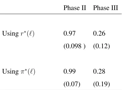
from INTEL’s annual reports.22 _{Table 4 reports the value ofϕestimated using the data from annual}

21_{Note that in referring to elasticity, I take absolute values, for example the elasticity ofm}∗_(ℓ)is|∂m∗(ℓ)

∂ℓ / m∗₍ℓ)

ℓ |.

22_{During the years in Phase II and Phase III, most of INTEL’s revenues and profits came from sales of}

reports. The elasticityϕdecreased from 0.97 in Phase II to 0.26 in Phase III when estimated from the revenue function r∗(ℓ), and from 0.99 to 0.28 when estimated from the gross profit function

π∗_{(ℓ), consistent with the hypothesis that there was a decrease inαin going from Phase II to Phase}

III. A change in α would also change π (see equation (8)) and hence the threshold lag x∗ (see equation 15) and possibly the choice of adoption policyn∗ _{and the scaling factorδ}n∗

. Similar to

the analysis for an unanticipated change inλabove, unless the change inαis sufficiently large, it will not lead to a change inn∗_{. As can be seen from Figure 4 the scaling factorδ}n∗

has not changed

between Phases II and III, suggesting again that n∗ did not change. If neither n∗ norλ changed in going from Phase II to Phase III, then the model predicts that the mean adoption interval n_λ∗ should not have changed either. This prediction is borne out in the data, the mean adoption interval was 2.03 years in Phase II, quite close to the 2.10 years in Phase III. Thus, the changes seen in the

data are consistent with what the model predicts should have been the response of INTEL to an increase inλin Phase I and a decrease inαin Phase II.

5.1

Decomposition of Changes in Growth of Performance

In this section, I quantitatively assess the contributions of changes inλ andα to the acceleration and slowdown. For two time periodstandt′, equation (16) implies that

gm_t′

gmt =

µ

λt′

λt

¶ µ

1 + 2αt′

1 + 2αt

¶

. (17)

sinceδis assumed to be the same across all periods. A change in the rate of technological progress,

gm_t′

gmt , can thus be neatly separated into contributions from the semiconductor equipment sector,

λt′

λt

,

and from INTEL, 1 + 2αt′

1 + 2αt

. The estimates of α and λ for the three periods, in conjunction with equation (17), can be used to quantitatively decompose the changes ingm. I estimate the value ofλ

for the three phases using data on adoption intervals,∆τj. Since∆τj ∼G(n∗,1_λ), the parameters

n∗ _{andλ can be estimated by the maximum likelihood method using the data on∆τ}

j. There are,

however, only 13 data points for∆τj, since INTEL has made just 14 adoptions in the period

1971-2008. Hence the sample for each phase considered separately is very small. Fortunately, the model provides a useful guideline to aid the estimation. The data on the scaling factor implies thatn∗_has

remained constant across the three phases (see stylized fact 1 and Figure 4). Hence I estimaten∗

using the data on∆τj pooled together from all three phases and use this value ofn∗ to estimateλ

for the three phases separately. For estimatingα, equation (6) implies thatαcan be obtained from the regression,ln (m) = constant+ (1 + 2α) ln (ℓ). The estimates ofλandαare given in Table 1. As can be seen from the table,λincreased after Phase I andαdecreased after Phase II.

Table 1: ESTIMATES OFλandα

Phase 1 Phase II Phase III

λ 0.92 1.96 1.90 (0.27) (0.47 ) (0.47)

α 0.53 0.78 0.14 (0.18) (0.10) (0.02)

Notes:λis given as the number of innovations per year.λis estimated using the maximum likelihood method from

the data on adoption intervals, which the model predicts to be distributed according to the gamma distribution

G(n∗_,1

λ). The parameterαis estimated from the regressionln (m) =constant+ (1 + 2α) ln (ℓ). Standard errors are shown in brackets. Standard errors forλwere estimated by bootstrapping, and are conditional onn∗_estimated

from the pooled sample.

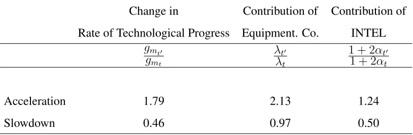
The decomposition of the acceleration and slowdown into contributions from the two sectors,

the corresponding sector did not play a role in the acceleration or slowdown. It can be seen from

the first row thatgm increased by a factor of 1.79 going from Phase I to II . The contribution from

semiconductor equipment industry increased by a factor of2.13and the contribution from INTEL increased by factor of1.24. Hence, the increase ingmwas caused overwhelmingly by an increase

in the innovation rate in the semiconductor equipment industryλ.23 _{The slowdown, however, was}

caused entirely by a decrease in INTEL’s own efficiencyα, as can be seen from the second row of Table 2.

Table 2: Decomposition of the Acceleration and Slowdown

Change in Contribution of Contribution of

Rate of Technological Progress Equipment. Co. INTEL

gm_t′

gmt

λt′

λt

1 + 2αt′

1 + 2αt

Acceleration 1.79 2.13 1.24

Slowdown 0.46 0.97 0.50

Notes:Equation (16) stipulates that the entries in the second column should equal the product of the entries in the

third and fourth columns. A value of 1 for the third or fourth column means that the corresponding sector did not play any role in the change ingm. As can be seen from the entries in the first row, the equipment firms played the

important role in the acceleration. For the slowdown on the other hand, INTEL was responsible and the equipment companies hardly contributed.

23_{The two contributions taken together account for more than the1.79factor increase in performance seen in the}

The finding that there was an increase in the innovation rate λ in the semiconductor equip-ment industry after Phase I has been corroborated in other studies, including Jorgenson (2001) and Aizcorbe et al. (2006), who report it in terms of a decrease in the time interval between the

adoption of new vintages. A possible explanation for the increase inλ, suggested in Hutcheson (2005), is that it was the outcome of R&D coordination activities in the semiconductor equipment

industry undertaken by SEMATECH, an industrial research consortia established in 1988. It re-mains a topic of further research to understand the cause of the increase in the innovation rate,

and to examine the possible role played by SEMATECH. On the other hand, there is widespread agreement in the semiconductor industry on the reason for the drop in efficiencyα, which caused the slowdown. In early 2000s, microprocessors with new designs introduced by INTEL hit a well publicized problem, the microprocessors generated a large amount of heat during their operation

which affected their proper functioning. Since then INTEL has abandoned the pattern of design improvements that it had followed in the past and adopted a new approach, the multicore design.

The multicore approach is less effective than previous approaches in translating increases in the number of transistors available on a microprocessor to increases in performance. This widely held

explanation has found its way even to the popular press, with the following quote coming from an article in the The New York Times - “The computer industry has a secret. Yes, the number

of transistors on modern microprocessors continues to multiply geometrically, but no one really knows how to get the most out of all these new transistors”. 24 _{The inability of INTEL’s designs to}

get the most out of the new transistors is captured in the model as a drop in the efficiencyα. Finally, it should be noted that although the explanations for the acceleration and slowdown

suggested here are based on shifts in model parameters, there are key relationships in the model that have not changed across the three phases. The scaling factor has remained roughly constant

across the three phases (see Figure 4). Similarly, the relationship betweenT andℓhas not changed

24_{The quote appeared in an article titled “Optimal Use of Transistors Still Elusive”, by John Markoff,}

across the three phases (see Figure 5).

6

Conclusion

This paper develops an economic model of the microprocessor industry that endogenizes techno-logical progress in the industry. The model captures well the evolution of different engineering and

economic variables in the industry and connects the engineering and economic measures of tech-nological progress. The model was used to understand the cause of the acceleration in

technolog-ical progress in the industry during 1990-2000 and the subsequent slowdown. Three conclusions emerge from this application of the model. First, the acceleration in technological progress was

driven by an increase in the innovation rate in the semiconductor equipment industry leading to more rapid adoption of innovations by INTEL. Second, the slowdown was caused by a decrease in

the efficiency with which INTEL was able to use the innovations generated by the semiconductor equipment industry. Third, innovation in the semiconductor equipment industry has been the main

workhorse driving technological progress in the microprocessor industry since 2001. However, further innovation in the semiconductor equipment industry is becoming ever more difficult as the

industry approaches the physical limit to reducing the size of the transistor. If innovations in the semiconductor equipment industry slows down, then it will accentuate the existing difficulties in

maintaining the rate of technological progress in the microprocessor industry.

References

Aizcorbe, Ana, “Moore’s Law, Competition, and Intel’s Productivity in the Mid-1990s,”American

Economic Review, May 2005,95(2), 305–308.

and Samuel Kortum, “Moore’s Law and the Semiconductor Industry: A Vintage Model,”

, Stephen D. Oliner, and Daniel E. Sichel, “Shifting trends in semiconductor prices and the pace of technological progress,” Finance and Economics Discussion Series 2006-44, Board of Governors of the Federal Reserve System (U.S.) 2006.

Balcer, Yves and Steven A. Lippman, “Technological expectations and adoption of improved technology,”Journal of Economic Theory, December 1984,34(2), 292–318.

Berglund, C. Neil, “A Unified Yield Model Incorporating Both Defect and Parametric Effects,”

IEEE Transactions on Semiconductor Manufacturing, August 1996,9(3), 447–454.

Blackwell, David, “Discounted Dynamic Programming,”Annals of Mathematical Statistics, 1965,

36, 226–235.

Borkar, Shekhar, “Design Challenges of Technology Scaling,”IEEE Micro, 1999,19(4), 23–29.

Condon, Stephanie, “Intel to Invest $7 Billion in U.S. Manufacturing Facilities,”CNET, February 10 2009. http://news.cnet.com/8301-13578 3-10160368-38.html.

Dixit, Avinash K. and Robert S. Pindyck, Investment under Uncertainty, Princeton University Press, 1994.

Doraszelski, Ulrich, “The net present value method versus the option value of waiting: A note on Farzin, Huisman and Kort (1998),”Journal of Economic Dynamics and Control, August

2001,25(8), 1109–1115.

Farzin, Y. H., K. J. M. Huisman, and P. M. Kort, “Optimal timing of technology adoption,”

Journal of Economic Dynamics and Control, May 1998,22(5), 779–799.

Flamm, Kenneth, “Moores Law and the Economics of Semiconductor Price Trends,” in Dale W. Jorgenson and Charles W. Wessner, eds., Productivity and Cyclicality in Semiconductors:

Goettler, Ronald and Brett Gordon, “Competition and Innovation in the Microprocessor Indus-try: Does AMD spur INTEL to innovate more?,” Working Paper 2009.

Gordon, Brett R., “A Dynamic Model of Consumer Replacement Cycles in the PC Processor Industry,”Marketing Science, September 2009,28(5), 846–867.

Gordon, Robert J., “Technology and Economic Performance in the American Economy,” NBER Working Papers 8771, National Bureau of Economic Research February 2002.

Griliches, Zvi, “Hybrid Corn: An Exploration in the Economics of Technological Change,”

Econometrica, 1957,25(4), 501–522.

Hoppe, Heidrun C., “The Timing of New Technology Adoption: Theoretical Models and Empir-ical Evidence,”Manchester School, January 2002,70(1), 56–76.

Hulten, Charles R., “Growth accounting with intermediate inputs,”The Review of Economic Stud-ies, October 1978,45, 511–518.

Hutcheson, Dan, “The R&D Crisis,” Technical Report, VLSI Research, Santa Clara 2005.

Jorgenson, Dale W., “Information Technology and the U.S.Economy,” American Economic

Re-view, 2001,91(1), 1–32.

Moore, Gordon E., “Cramming More Components onto Integrated Circuits,”Electronics, April 1965,38(8).

, “Progress in Digital Integrated Electronics,”IEEE, IEDM Technical Digest, 1975, pp. 11–

13.

Oliner, Stephen D. and Daniel E. Sichel, “Information technology and productivity: where are we now and where are we going?,” Finance and Economics Discussion Series 2002-29, Board of Governors of the Federal Reserve System (U.S.) 2002.

and , “The Resurgence of Growth in the 1990s: Is Information Technology the Story?,”

Journal of Economic Perspectives, 2002,2000(14), 3–22.

, , and Kevin J.Stiroh, “Explaining a Productive Decade,” Finance and Economics Discussion Series 2007-63, Board of Governors of the Federal Reserve System (U.S.) 2007.

Pakes, Ariel and Paul McGuire, “Computing Markov-Perfect Nash Equilibria: Numerical Impli-cations of a Dynamic Differentiated Product Model,”RAND Journal of Economics, Winter

1994,25(4), 555–589.

Ronen, Ronny, Avi Mendelson, Konrad Lai, Shih-Lien Lu, Fred Pollack, and John P. Shen, “Coming Challenges in Microarchitecture and Architecture,”Proceedings of the IEEE, 2000,

89(3), 325–340.

Semiconductor-International, “VLSI Research Ranks Top Equipment Vendors for 2007,”

www.semiconductor.net/article/CA6541940.html, 2008.

Stokey, Nancy L, Robert E Lucas, and Edward Prescott, Recursive Methods in Economic

Dy-namics, Harvard University Press, 1989.

7

Mathematical Appendix

Proposition 1 The optimal policy of the firm is to wait until the lag behind the frontier,x = ℓ_ℓ¯, reachesx∗, where

x∗ =

½µ

ρ+λ− λ

δϕ

¶ µ

v(1)−F(1)

π

¶¾_ϕ1

Proof. Equation (13) can be rewritten as

v(x) = π

ρ+λx

ϕ

+ 1

δϕ λ

ρ+λ[M ax{v(δx), v(1)−F(1)}]

wherex∈(0,1]. Consider operator,T that maps functions defined on(0,1]as

T(f(x)) = π

ρ+λx

ϕ₊ 1

δϕ λ

ρ+λ[M ax{f(δx), f(1)−F(1)}]

T(.) maps continuous functions to continuous functions. Moreover, it is easily seen from the conditions in Blackwell (1965) that T is a contraction mapping. Hence by contraction mapping theorem there exists a unique v(x) that solves the Bellman equation above. Moreover, T maps weakly increasing functions to strictly increasing functions, hencev(x)is strictly increasing (see Stokey, Lucas and Prescott (1989)). Hence, there exists a valuex∗ such that

v(x∗) =v(1)−F(1). (18)

Moreover, sincev(.)is an increasing function andδ <1

v(δx∗)< v(1)−F(1). (19)

Evaluating the Bellman equation (7) atx=x∗ and using equations (18) and 19 gives,

v(x∗) = π (ρ+λ)x

∗ϕ

+ 1

δϕ λ

(ρ+λ)M ax{v(δx

∗_{),[v(1)−F(1)]}}

v(1)−F(1) = π

(ρ+λ)x

∗ϕ

+ 1

δϕ λ

ρ+λ[v(1)−F(1)]

which gives

x∗ =

½µ

ρ+λ− λ

δϕ

¶ µ

v(1)−F(1)

π

Lemma 2 If∆τi ∼G(n∗,1_λ), thenE

£

e−ρ∆τi¤ =

³

λ

ρ+λ

´n∗

Proof. SinceG(n∗,_λ1) = λn

∗

∆τjn

∗₋₁

e−λ∆τ j

Γ(n∗

) , whereΓ(n

∗_{) = (n−1)!is the Gamma function,}

E£e−ρ∆τi¤ ₌

Z ∞

0

e−ρtλ

n∗

∆τn∗

−1_e−λT

Γ(n∗₎ d∆τ =

λn∗

Γ(n∗₎

n∗₋₁

ρ+λ

Z ∞

0

∆τn∗−2e−(ρ+λ)∆τd∆τ

=

µ

λ ρ+λ

¶n∗

(n∗−1)! Γ(n∗₎ =

µ

λ ρ+λ

¶n∗

Proposition 3 Given the innovation rate λ, the expected present discounted value of adopting everynthinnovation is

¯

V(n, λ) = _¯1

ℓϕ₀



 

n

1−³_ρ+λ_λ´noπ_ρ −³_δ1ϕ_ρ+λ_λ

´n

F(1) 1−³_δ1ϕ_ρ λ

+λ

´n



 

Proof. Let{∆τj}∞_j=0 be the adoption intervals. Then theith adoption with vintageℓi = (δn)iℓ¯0,

occurs at timeτi =

i−1

X

j=0

∆τj. Then if the firm follows the policy of adopting everynth innovation,

the net profit of the firm in the ith adoption interval (i.e the profit from operating the ith vintage equipment), discounted back tot= 0is,Πi(n, λ) =

e−ρτi

½Z ∆τi

0

e−ρt π

(δniℓ¯0)ϕ

dt− F(1) (δniℓ¯0)ϕ

¾

=e

−ρ

i−1

X

k=0

∆τk 1

δniϕℓ¯0

½

π ρ

¡

1−e−ρ∆τi¢_−F(1)

¾

Then the present discounted value of net profits obtained under the policy of adopting every nth

innovation is

∞ X

i=0

Πi(n, λ), which is given by

∞ X

i=0

Πi(n, λ) =

1 ¯

ℓϕ₀

      ∞ X i=0 1

δniϕe

−ρ

i−1

X

k=0

∆τk

π ρ − ∞ X i=1 1

δniϕe

−ρ

i−1

X

k=0

∆τk

F(1)−

∞ X

i=0

1

δniϕe

−ρ i

X

k=0

∆τkµ

ThenV¯(n, λ) = E

∞ X

i=0

Πi(n, λ)

= _¯1

ℓϕ₀

      ∞ X i=0 1

δn∗iϕ π ρE[e

−ρ

i−1

X

k=0

∆τk

] −

∞ X

i=1

1

δn∗iϕF(1)E[e

−ρ

i−1

X

k=0

∆τk ] − ∞ X i=0 1

δn∗iϕ

µ

π ρ

¶

E[e

−ρ i

X

k=0

∆τk ]      

The adoption interval ∆τj is the time taken for n∗ poisson events to happen. Hence ∆τj are

independent draws from the Gamma distributionG_(n∗_, 1

λ). It follows that

Pi−1

j=0∆τj ∼G(n∗i,_λ1).

To evaluate the above expectations, I use Lemma 2, which shows thatE£e−ρ∆τi¤=

³

λ

ρ+λ

´n∗

. This implies

¯

V(n, λ) = E

∞ X

i=0

Πi(n, λ)

= _¯1

ℓϕ₀

" _∞ X

i=0

1

δn∗iϕ π ρ

µ

λ ρ+λ

¶n∗i

−

∞ X

i=1

1

δn∗iϕF(1)

µ

λ ρ+λ

¶n∗i

−

∞ X

i=0

1

δn∗iϕ

µ

π ρ

¶ µ

λ ρ+λ

¶n∗(i+1)#

Evaluating the sums of geometric series, the above expression reduces to

¯

V(n, λ) = E

∞ X

i=0

Πi(n, λ) = 1 ¯

ℓϕ₀



 

n

1−³_ρ+λ _λ´noπ_ρ −³ 1

δϕρ+λλ

´n

F(1) 1−³_δ1ϕ_ρ λ

+λ

´n



 

8

Data Sources

microprocessors for INTEL. I omitted the server processors manufactured by INTEL since

func-tionally they are very different from desktop and laptop microprocessors, which form the focus of this paper. The data form was obtained from two sources - Standard Performance Evaluation Corporation (SPEC) and Business Applications Performance Corporation (BAPCo). SPEC and BAPCO are industry consortia of which both microprocessor producers, INTEL and AMD, are

9

Appendix

Phase−I Phase−II Phase−III

0

.1

.2

.3

.4

.5

.6

.7

.8

.9

1

Scaling Factor

10 6 3 1.5 1 .8 .6 .35 .25 .18 .13 .09 .065 .045 Vintage (l)

Scaling Factor of Transistor Size at each Vintage Adoption

Phase−I Phase−II Phase−III

.1

1

10

100

1000

10000

Transistors (millions)

10 6 3 1.5 1 .8 .6 .35 .25 .18 .13 .09 .065 .045 Vintage (l)

Transistor Evolution with Vintage (slope=2.34)

0 0.5 1 1.5 2 20

25 30 35 40 45 50 55 60

n*=3 n*=4 n*=5

λ

V(n,

λ

)

n=3 n=4 n=5

Figure 6: Variation ofn∗ _withλ

Notes:The y-axis variable,V¯(n, λ)is the present discounted value of the firm if it adopts everynth

innovation, given arrival rateλ. The optimal adoption policyn∗_{is the value ofnthat maximizesV}¯_{(n, λ). As can be seen from the}

Table 3: RATE OF TECHNOLOGICAL PROGRESS IN MICROPROCESSOR INDUSTRY

Company Annual Performance Growth Rate(%)

1971-1989 1990-2000 2001-2008

INTEL 28.4 50.2 22.9

AMD 10.9 65.4 18.5

Source: Author

Annual Hedonic Price Index Decline Rate(%)

1988-1994 1994-2001 2001-2004

Industry 30.0 63.1 40.5

Source: Aizcorbe et al. (2006)

Notes:The top panel shows the average growth rate of microprocessor performance during the three phases. The

Table 4: ESTIMATES OFϕFROM THE REVENUE FUNCTION AND GROSS PROFIT FUNC-TION

Phase II Phase III

Usingr∗(ℓ) 0.97 0.26 (0.098 ) (0.12)

Usingπ∗_{(ℓ) 0.99 0.28}

(0.07) (0.19)

Notes:The first row showsϕestimated from the equationln(r∗_{) =constant+ ln(ℓ). The data for revenues were}

taken from INTEL’s annual reports. The average annual revenue over the years of operation of a vintageℓis taken as

r∗_{(ℓ). The years of operation of a vintageℓis taken to be the years between the year in whichℓwas adopted to the}

Table 5: IMPACT ON AGGREGATE PRODUCTIVITY GROWTH

Phase Output Share TFP Growth Contribution of Microprocessors

of Microprocessors in Microprocessor to Aggregate TFP Growth (%) Industry (%) (% points)

1971-1989 0.06 28.4 0.017

1990-2000 0.14 50.2 0.070

2001-2008 0.13 22.9 0.031

Notes:The output share is obtained by multiplying the output share of semiconductors given in Oliner and Sichel