Spatial modelling and volatility matrix estimation in high dimension statistics with financial applications

(1)

Spatial Modelling and Volatility Matrix

Estimation in High Dimension Statistics with

Financial Applications

Cheng Qian

The Department of Statistics

London School of Economics and Political Science

A thesis submitted for the degree of

Doctor of Philosophy

(2)

(3)

Declaration

I certify that the thesis I have presented for examination for the PhD degree of the London School of Economics and Political Science is solely my own work other than where I have clearly indicated that it is the work of others (in which case the extent of any work carried out jointly by me and any other person is clearly identified in it).

I confirm that Chapter 1 and 3 were jointly co-authored with my su-pervisor, Dr.Clifford Lam and Chapter 2 was jointly co-authored with Dr.Clifford Lam and Professor Hui Wang from Central University of Finance and Economics, China.

(4)

Acknowledgements

First of all, I would like to thank my supervisor, Dr.Clifford Lam, for this constant help, patient guidance and professional advice for my PhD research and life. Without him, it is impossible that I can finish my PhD study early and pursue a postdoc in the following two years.

(5)

Abstract

High dimension modelling is an important area in modern statistics. For example, a large number of problems that arise in finance are also in-spired by more and more available high dimensional data. The main objective of this thesis is to investigate three methodologies in high di-mension statistics with the application in finance. The subsequent chap-ters are organized as follow. The first two chapchap-ters are about spatial modeling and its inference respectively. The third chapter tackles a dif-ferent problem about the estimation of large integrated volatility matrix of high frequency data.

In the first chapter, a dynamic spatial model with different weight matri-ces for different time-lagged spatial effects is proposed. Unlike assuming a known spatial weight matrix, the proposed method estimates each spa-tial weight matrix for corresponding spaspa-tial effect by a linear combination of a set of specified spatial weight matrices to avoid misspecification. To estimate the coefficients for linear combinations and covariates, the pro-filed least square estimation is used with instrumental-like variables. A further selection on spatial weight matrices is introduced by adding an adaptive LASSO penalty on the coefficients of linear combination. All theoretical results are built on the scenario when the sample size T and panel dimension N go to infinity. The functional dependence in time se-ries proposed by Wu (2005) is applied for the asymptotic normality of the estimated parameters. The oracle properties for model selection are de-veloped including the asymptotic normality and sign consistency. Apart from a simulated data used to illustrate the performance of the proposed model, we also apply the proposed model to 32 important stocks from the Euro Stoxx 50 and S&P 500 in 2015 to invest the spatial interaction of them.

(6)

quasi-in our model and their consistency and asymptotic normality are estab-lished when both N and T are large. Using the asymptotic normality of the quasi-maximum likelihood estimators, a Wald test can be em-ployed on the coefficients of the linear combination. Then, a diagnostic test proposed in Chang et al. (2017) is applied to test whether the fit-ted residuals perform like a white noise vector in our large N and large T setting. Simulated and real data are used to demonstrate the per-formance of the proposed quasi-maximum likelihood estimation and all above tests.

The third chapter is about the estimation of large integrated volatility matrix for high frequency data. Besides the microstructure noises and non-synchronous trading times for high frequency data analysis should be fixed, the bias in the extreme eigenvalues coming from the high di-mensionality are also not negligible. A nonparametric eigenvalue regu-larization proposed in Lam (2016) is applied on three existing volatility matrix estimators, such as multi-scale, kernel and pre-averaging realized volatility matrix estimators. One advantage for the proposed estimators is no need for implicit assumptions on the structure of the true integrated volatility matrix. It can be proved that the bias in the extreme eigenval-ues can be shrunk and the regularized volatility estimators are positive definite in probability. Incidentally, the bias-corrected versions of kernel and pre-averaging estimators, which have faster rate of convergence at n−1/4 _{but are not guaranteed to be positive definite in Barndorff-Nielsen}

(7)

List of Figures

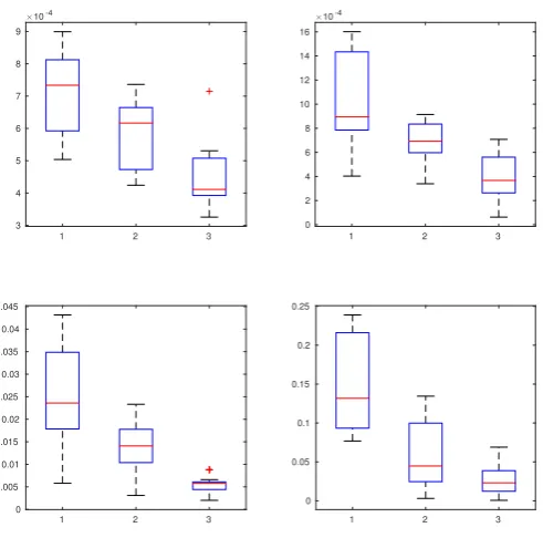
1.1 Boxplots of averagedL1 errors. Upper row: P3_i₌₁|βb_i−β_i|/3. Bottom

row: bδ−δ

1/9. Left column (from left to right): N = 40,80,120, T =

60. Right column (from left to right): T = 40,80,120, N = 60. . . 28 1.2 Histograms and normal probability plots for standardized ˆβ1 (upper

row) and ˆδ1,3 (lower row) with N = T = 80. Standardization used

respectively the asymptotic results from Theorem 2 and 3. . . 28 1.3 Upper: The estimate ofW0. Lower: The estimate ofW1. From 1 to

32, the stocks are Alstom, Total, BNP, Scociete, Sanofi, Carrefour, LVMH, Vivendi, Daimler, Allianz, Deutsche Bank, ENEL, ENI, In-tesa, Unicredit, Tele Italy,Repsol, Banco, Telefonica, GM, PG, Nex-tera, American Express, Citi, Wells Frago, Amgen, Gilead, Johnson, Costco, Home, Centurylink and Verizon respectively. . . 34

2.1 Boxplots of kθˆN T − θ0k1/11. Left panel, from left to right: N =

50,100,150, T = 100. Right panel, left to right: T = 50,100,150, N = 100. . . 76 2.2 Histograms (left) and normal probability plot (right) for standardized

ˆ

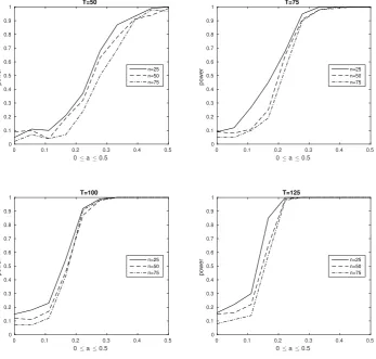
σ2. Standardization used the estimated asymptotic covariance matrix derived in Theorem 2. . . 76 2.3 Power curves for the diagnostic test in Section 2.6 with 0≤ a ≤0.5

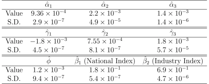
for different (N, T) combinations. Significance level is set at 5% in all cases, withK = 10 lags considered. . . 79 2.4 Upper: The matrix P3

i=1αˆiWi. Lower: The matrix

P3

(11)

3.1 Boxplots of Frobenius errors of NER-TSRVM, TSRVM, NER-MSRVM, MSRVM, NER-KRVM, KRVM, NER-PRVM and PRVM for C = 0. The upper plot is for no jump scenario, while the bottom one is for jumps model (sd=1/30) result. . . 132 3.2 Boxplots of Frobenius errors of MSRVM and mMSRVM with

non-parametric regularization forC = 0. . . 132 3.3 Boxplots of Frobenius errors of positive semi-definite estimators

pKRVM and NER-pPRVM) and bias-corrected estimators (NER-KRVM and NER-PRVM) forC = 0. . . 133 3.4 Boxplots of Frobenius errors of NER-PRVM, PR-POET and POET

forC = 0. . . 133 3.5 Boxplots of Frobenius errors of TSRVM, MSRVM, KRVM, PRVM

and their nonparametric regularization estimators for C = 1. The upper plot is for no jump scenario, while the bottom one is for jumps model (sd=1/30) result. . . 134 3.6 Boxplots of Frobenius errors of MSRVM and mMSRVM (scale is 1/2)

with nonparametric regularization for C= 1. . . 134 3.7 Boxplots of Frobenius errors of positive semi-definite estimators

pKRVM and NER-pPRVM) and bias-corrected estimators (NER-KRVM and NER-PRVM) forC = 1. . . 135 3.8 Boxplots of Frobenius errors of NER-PRVM, PR-POET and POET

forC = 1. . . 135 3.9 Simulation results about microstructure noise effect by Frobenius

er-rors for model 3.2 without factors (C = 0) and with factors (C = 1) from the upper to the bottom but no jumps. . . 136 3.10 Simulation results about dimension p effect by Frobenius errors for

(12)

Chapter 1

Spatial Lag Model with

Time-lagged Effects and spatial

weight Matrix Estimation

1.1

Introduction

There are always complicated correlation over cross section and time in the real data. In econometrics, spatial econometrics develop the models to investigate the cross-sectional interactions. For example, spatial autoregressive model proposed in Cliff and Ord (1973) is very powerful. Among these models, Anselin et al. (2008) divides them into four groups. The first type is “pure space recursive” if only a spatial time lag is included. The second type is “time-space recursive” if both an individual time lag and a spatial time lag are included. The third type is “time-space simultaneous” if an individual time lag and a contemporaneous spatial lag are specified. And finally, the last type is “time-space dynamic” if all forms of lags are included. Besides the spatial autoregressive model, spatial disturbance autoregressive model is considered in Elhorst (2005). All these models have been frequently used well in many fields like regional markets in Keller and Shiue (2007), labour economics in Foote (2007) or public economics in Franzese and Hays (2007), to name but a few areas.

(13)

correct choice of spatial weight matrix whose elements reflect the strength of inter-action among units in the panel. In plenty of applications of spatial autoregressive model, the spatial weight matrix is assumed as a prior knowledge. Physical distance between two units in the panel is often regarded as the inverse measurement of the interaction between them, so people used−1 _{as the entry of the spatial weight matrix}

where d is the corresponding distance. Naturally, physical distance is not the only choice for the cross sectional interaction measurement. For example, in economics, two countries from a same economic organization may have a strong relation in spite of far distance between them. Even if only considering the physical distance, d−2

or d−3 _{can also be the candidates. Therefore, it is limited to only use one spatial}

weight matrix into the model. Corrado and Fingleton (2012) also criticizes the spa-tial econometrics due to this misspecification of spaspa-tial weight matrix. In Lam and Souza (2015b), an error upper bound is given for the estimation of spatial regres-sion parameters, which shows that misspecification of the spatial weight matrix can introduce large bias in the final estimates.

(14)

weight matrix involved is estimated by a linear combination of user-specified spatial weight matrices. A similar model in Lee and Liu (2010b) is named as high order spatial autoregressive model. The inclusion of more than one spatial weight matri-ces can allow spatial dependence from different interaction characteristics such as geographical contignity and economic interaction. Therefore, it helps to avoid the risk of misspecification of the spatial weight matrices, while maintaining the overall parsimony of the model.

As for the high order spatial autoregressive model, Lee and Liu (2010b) and Lee and Yu (2014a) propose the generalized method of moments estimation. However, as discussed in Li (2017), when we have a large or moderately large sample size T, the generalized method of moments gets into trouble of “many moments bias” as the number of moment conditions also increases dramatically. This point is also men-tioned in Lee and Yu (2014a) that generalized method of moments requires careful analysis when T → ∞. Another solution for the high order spatial autoregressive model is quasi-maximum likelihood estimation introduced in Yu et al. (2008) and Li (2017). But it is well known that quasi-maximum likelihood estimation is not practical and computationally infeasible because of the complex parameter space and the difficulty in Jacobian determinant evaluation, especially for the proposed model in this chapter that includes p time-lagged spatial effects.

Therefore, it is prefered to find an efficient estimation but no complicated parameter space is involved. Therefore, the profiled least square estimation is applied for the coefficients of linear combinations and covariates. Meanwhile, the innate endogene-ity in our time-lagged spatial model causing least square type estimation inconsistent can not be ignored. To overcome this difficulty, we introduce instrument-like vari-ables. In the particular case when the covariates are exogenous, they themselves can act as these instrument-like variables. We estimate the “best” linear combination for each required spatial weight matrix, then an adaptive LASSO can be applied for highlighting the relative contributions of each specified one. The convergence and asymptotic normality of all estimators are presented under the functional de-pendence measurement of time series variables in Wu (2005) or Wu (2011), allowing both the sample sizeT and the panel size N to grow to infinity together. As shown in our real data analysis, with the input of different specified spatial weight matrices, the scope of applications of our model is expanded since there are numerous ways to specify a spatial weight matrix.

(15)

and some relative further studies are listed in Section 1.7. All the technical proofs are relegated to the Section 1.8.

1.2

Methodology

1.2.1

The Model

Consider the following dynamic spatial lag model

y_t=µ+W0yt+W1yt−1+· · ·+Wpyt−p+Xtβ+t, t= 1, . . . , T, (1.1) where y_t = (yt1, yt2, ..., ytN)T is an N ×1 vector of observed time series variables and µ is an N ×1 constant vector. The data starts from y₁_−p, and hence the true sample size is T +p. It does not affect our asymptotic analysis since p is finite in this paper. Hereafter when we talk about the sample size, we useT instead ofT +p for simplicity. Forj = 0,1, . . . , p, Wj is an N ×N spatial weight matrix with 0 on the main diagonal, which model the simultaneous and dynamic interaction between different unit in the panel. To capture the dynamic interaction between same unit, the N ×K matrix of covariates Xt can contain yt−j for j = 1, . . . , p in its columns on top of other covariates, while β is the K ×1 vector of regression coefficients. The series{t} is an innovation process with mean0and covariance matrixΣ. For more detailed assumptions, see Section 1.8.1.

In many applied spatial econometrics applications,W0 is assumed known and there

are no lagged terms Wjyt−j for j = 1, . . . , p. Instead of assuming all the spatial weight matrices are known, in this paper we assume that there are M specified spatial weight matrices W0i, i = 1, . . . , M, such that each spatial weight matrix is a linear combination of the M specified ones. This is motivated by the fact that there are often more than one measures of spatial interactions. For instance, for the geographical distance r alone between two specific locations, we can specify three different entries r−1_, _r−2 _and _r−3_{, creating three specified spatial weight matrices.}

These are indeed our distance specifications included in our data application in Section 1.6. Spatial contiguity is also another popular choice in spatial econometrics. The linear combination for each Wj is written as

Wj = M

X

(16)

where δji for i = 1, . . . , M, j = 0, . . . , p are unknown coefficients in the proposed model.

Apart from allowing for estimating the spatial weight matrices from pre-specified ones, our model also includes time-lagged spatial effects. In a differently specified spatial lag model, Dou et al. (2016) includes one lag to reflect such effects. We generalize this to p time-lagged effects, with p to be determined by data driven methods as described in Section 1.4. The pure dynamic effects are captured by the term Xtβ, since we can allocate {yt−1, . . . ,yt−p} to be the columns in Xt, so that then K ≥ p, and K = p if no other covariates are present. Not counting the parameters in µ, there are K+M(p+ 1) parameters to be estimated in total. With µ, the spatial fixed effects of the model is then (IN −W0)−1µ. For

iden-tifiability of such, we assume without loss of generality that _E(Xt) = 0. As the instrumental variable deducts its mean in our methodology, the non-zero µ can be removed. Therefore, our assumption _E(Xt) = 0 is same as E(yt) = 0. If we do not have_E(Xt) = 0, we can write

Xtβ+µ= (Xt−E(Xt))β+ (µ+E(Xt)β)

so that the spatial fixed effects are now captured byµ+_E(Xt)β rather than µ.

1.2.2

Profiled least square estimation with endogeneity

The first important problem needed to be concerned is the endogeneity in model (1.1). To estimate β and δ more efficiently, we assume that there are variables Bt of size N×K such that they are correlated with Xt but independent of tfor each t = 1, . . . , T. In particular, if Xt is exogenous, we can set Bt =Xt. To apply the instrument-like variableBt in the vectorized model, we first define

B=T−1/2N−a/2(Bζ−Bζ) =T−1/2N−a/2IN⊗ {(IT⊗ζT)(B1−B¯, . . . ,BT−B¯)T},

where ¯B =T−1PT

t=1Bt, ζ =K

−1₁

(17)

UsingBto avoid the inconsistency from endogeneity, we first rewrite (1.1) to present our model more neatly as

y =µ⊗1T +Z0V0δ0+Z1V0δ1+· · ·+ZpV0δp+Xβvec(IN) +,

where y= vec(y₁, . . . ,y_T)T, = vec(1, . . . ,T)T, Zj =IN ⊗(y1−j, . . . ,yT−j)T and

δj = (δj1, δj2, . . . , δjM)T for j = 0,1, . . . , p, Xβ = IN ⊗(IT ⊗βT)(X1, . . . ,XT)T, and V0 = (vec(WT01), . . . ,vec(W

T

0M)). The notation ⊗ is the Kronecker product, and 1T defines a vector of ones with size T. Simplifying, we have

y=µ⊗1T +ZV δ+Xβvec(IN) +, (1.2) whereZ = (Z0, . . . ,Zp),δ = (δT0, . . . ,δ

T

p)T, andV =Ip+1⊗V0. Then, multiplying

BT on both sides of (1.2), we arrive at the augmented model

BTy =BTZV δ+BTXβvec(IN) +BT. (1.3) The constant term disappears sinceBT(µ⊗1T) = 0. Removing theN-dimensional constant term makes estimation much easier, while the error term BT is now weaker in correlations with the design matrixBTZV, so that least square estimation becomes viable again.

After introducing B serving as instrumental variable, same as Lam and Souza (2018), we can apply profiled least square estimation on the augmented model to avoid the nonlinearity and to reduce variance if we estimateβandδ simultaneously. More specifically, to profile outβ and estimateδ, we rewrite the augmented model as

BvTyv₀ =BvT( M

X

i=1

δ0iW⊗0i)y v

0+B

vT p

X

j=1

( M

X

i=1

δjiW⊗0i)y v j +B

vT_Xβ₊_BvTv_,

where yv

j = (y1T−j, . . . , yTT−j)T for j = 0,1, . . . , p, v = (T1, . . . ,TT)T, B

v _{= ((}_B

1 −

¯

B)T_{, . . . ,}₍_B

T−B¯)T)T,X = (XT1, . . . ,X

T

T)T andW ⊗

0i =IT⊗W0i fori= 1, . . . , M. Assumingδ is known, we can estimate β by the least squared method, resulting in

β(δ) = (XTBvBvTX)−1XTBvBvTn(IT N − M

X

i=1

δ0iW⊗0i)y v

0−

p

X

j=1

( M

X

i=1

δjiW⊗0i)y v j

o

.

(18)

This formula provides a basis for a profile least square estimator forδ. We can show that by substituting the above into the augmented model (1.3), the profile least square estimator for δ is

ˆ

δ ={(H−BTZV)T(H−BTZV)}−1₍_H₋_BT_ZV₎T₍_K_yv

0 −B

T_y_), _(1.5) where

K =T−1/2N−a/2( T

X

t=1

Xt⊗(Bt−B¯)ζ)(XTBvBvTX)−1XTBvBvT,

H =KW⊗₀₁, . . . ,W⊗₀_M(IM ⊗yv0,IM ⊗y1v, . . . ,IM ⊗yvp). Therefore, with ˆδ, the profile least square estimator of β is given by

ˆ

β=β(ˆδ) = (XTBvBvTX)−1XTBvBvTn(IT N− M

X

i=1

ˆ

δ0iW⊗i )y v

0−

p

X

j=1

( M

X

i=1

ˆ

δjiW⊗i )y v j

o

.

(1.6) Finally, to estimate µ, we can use

ˆ

µ=IN − p

X

j=0

c

Wj

¯

y−X¯βˆ, where Wc_j =

M

X

i=1

ˆ δjiW0i.

The corresponding spatial fixed effects estimator is then given by (IN −Wc₀)−1µˆ.

1.2.3

Selection of specified spatial weight matrices

As the specified spatial weight matricesW0iare arbitrary, it is not necessary that all of them should be included. Since bδ is a least square-type estimator, each element

in it is not estimated to be exactly 0 in general. This hinders the selection of the specified spatial weight matrices, which is important for us to see which one truely contributes to the overall spatial weight matrix and which one does not. Especially, the different time-lagged spatial effects shown by the corresponding spatial weight matrixWj can have the different selection on the specified spatial weight matrices. It is true that some spatial characteristics can have the delayed impact, which is also reflected by our real data example in Section 1.6.

(19)

Souza (2018), the tuning parameter used in LASSO is same for all element, which causing excessive penalization by larger tuning parameter or insufficient penaliza-tion by smaller tuning parameter. To resolve this, Zou (2006) propose a method named adaptive LASSO. On the other hand, compared with SCAD penalty pro-posed in Fan and Li (2001), adaptive LASSO still enjoys convexity. Therefore, it has computational efficiency and can apply the same algorithm as standard LASSO. To handle the selection of specified spatial weight matrices, we apply the penalized profiled least square estimator eδ for δ same as the way used in Lam and Souza

(2018), with

˜

δ = argmin

δ

1 2TkB

T_y₋_BT_{ZV δ}₋_BT_X

β(δ)vec(IN)k2+γTuT|δ|, (1.7)

where u = (|δb₀_,₁|−1, . . . ,|δb₀_,M|, . . . ,|δb_p,₁|−1, . . . ,|bδ_p,M|−1)T, and |δ| represents the

same vectorδ with all its entries taken absolute value. The penalty term in (1.7) is similar to the adaptive LASSO proposed in Zou (2006), which shows a better per-formance in model selection than standard LASSO. A more direct penalized least square formulation is given by

e

δ = argmin

δ

1 2TkB

T_y₋₍_BT_ZV ₋_H₎_δ₋_g_k2₊_γ

TuT|δ|, where

g =T−1/2N−a/2( T

X

t=1

Xt⊗(Bt−B¯)ζ)(XTBvBvTX)−1XTBvBvTyv.

The tuning parameter γT can be found in Assumption R6 in Section 1.8. For choosing an appropriate γT in practice, see Section 1.4.2.

1.3

Theoretical Properties

We define some notations first before we present the time dependence measurement from Wu (2005) and our theoretical properties of all estimators. Compared with classic mixing condition, Wu (2005) discusses that, for stationary causal processes, the calculation of probabilistic dependence measures is generally not easy because it involves the complicated manipulation of taking the supremum over two sigma algebras. Additionally, many well-known processes are not strong mixing.

(20)

and {Xt}respectively, both with length N K. For t= 1, . . . , T, we assume that

xt={fj(Ft)}1≤j≤N K, bt={gj(Gt)}1≤j≤N K, t ={hl(Ht)}1≤l≤N,

where thefj(·),gj(·) andhl(·) are measurable functions defined on the real line, and let the shift processFt = (..., ex,t−1, ex,t),Gt= (..., eb,t−1, eb,t) andHt= (..., e,t−1, e,t) are defined by independent and identically distributed processes {ex,t}, {eb,t} and {e,t} respectively, with {eb,t} independent of {e,t}but correlated with {ex,t}. To build the asymptotic normality results for the estimators, we apply the functional dependence measure introduced in Wu (2005) for gauging the serial dependence of a process. For d >0, define

θ_t,d,jx =kxtj −x0tjkd= (E|xtj−x0tj| d₎1/d_, θ_t,d,jb =kbtj−b0tjkd= (E|btj−b0tj|d)1/d,

θ_t,d,l =ktl−0tlkd= (E|tl−0tl| d

)1/d,

where j = 1, ..., N K, l = 1, ..., N and x_tj0 =fj(Ft0),F 0

t = (..., ex,−1, e0x,0, ex,1, ..., ex,t), with e0_x,₀ independent of all other ex,j’s. Hence x0tj is a coupled version of xtj with ex,0 replaced by an independent and identically distributed copy e0x,0. Intuitively, a

large θx

t,d,j means that serial correlation is strong at least for variables at most time t apart. Finally, we have similar definitions for b0_tj and 0_tl.

1.3.1

Main assumptions

We introduce some assumptions for our theorems to hold. First, we denote the L1

normkvk1 =

PN

i=1|vi|for a N×1 vector v whose ith element is vi. More technical assumptions are moved to Section 1.8 to help the flow of this chapter.

M1. The elements in all Wi’s can be negative and Wi itself can be asymmetric. Moreover, definingS ={s= 1, . . . , K|The sth column of Xt contains yt−l, l = 1, . . . , p}, we assume PM

i=1|δ0i|<1 and

Pp

j=1

PM

i=1|δji|+

P

s∈S|βs|<1. M2. The processes {Bt}, {Xt} and {t} are second-order stationary, with {Xt}

(21)

M3. Define

Θx_m,a= ∞

X

t=m max

1≤j≤N Kθ x t,a,j, Θ

b m,a=

∞

X

t=m max

1≤j≤N Kθ b t,a,j, Θ

m,a=

∞

X

t=m max

1≤j≤Nθ t,a,j.

Then we assume that for some w > 2, Θx_m,₂_w,Θb_m,₂_w,Θ_m,₂_w ≤ Cm−α with α, C >0 being constants that can depend on w.

M4. (Identification condition) Assume that the two sets of parameters (δ∗,β∗) and (δo,βo) both satisfy the proposed model (1.2). Writeδ = (δ`)1≤`≤M(p+1), and

define the setH to be

H ={` :δ_`∗ 6= 0 or δo_` 6= 0}.

Then the identification condition is that the matrixOTOhas all its eigenvalues uniformly bounded away from 0, where

O = (T−1/2_E(BTZVH), T−1/2E(BTX˜)), and ˜

X = (x1,1, . . . ,xT ,1, . . . ,x1,N, . . . ,xT ,N)T.

The notation AH means that the matrix A has columns restricted to the set H, whilexT

t,j is thejth row of Xt.

Assumption M1 ensures that our model has a reduced form

y_t=Πµ+ΠW1yt−1+· · ·+ΠWpyt−p+ΠXtβ+Πt, Π= (IN−W)−1, t= 1, . . . , T. The matrixΠexists with the assumptionPM

i=1|δ0i|<1. Since row-standardization

meansW₀_i

∞ = 1, the condition

Pp

j=1

PM

i=1|δji|+

P

s∈S|βs|<1 implies that each

W_j

∞ <

PM

i=1|δji|

W₀_i

∞ < 1. At the same time, without loss of generality assuming S =φ and writing the model as

Φ(L)y_t=Πµ+ΠXtβ+Πt, Φ(L) = (IN −ΠW1L− · · · −ΠWpLp),

where L is the lag operator, then stationarity is ensured if det(Φ(z)) = 0 has all roots lying outside the unit circle. This is ensured by the conditionPp

j=1

PM

i=1|δji|+

P

(22)

The Assumption M2 and M3 are also used in Lam and Souza (2018). The indepen-dence between{Bt} and {t} in M2 ensures that {Bt} serves a function similar to an instrument for model (1.2). More details about the dependence between {Bt} and {Xt}are shown in Assumption R3 and R4 in Section 1.8.1.

The tail condition in M2 implies that all the random variables involved are with sub-exponential tails, which is a relaxation to strict normality. The different constants for{Bt},{Xt} and{t}process are finally dominated by the maximum one among them. Therefore, to simplify, we assume they are same in our proof.

Similar to Definition 3 in Wu (2005) for stability measurement, Θx

m,2w ≤ Cm−α in M3 essentially means that the strongest serial dependence for the xtj’s with at least m time units apart is decaying polynomially as m increases. It allows for the application of a Nagaev-type inequality in Lemma 1 in the Section 1.8 for our results to hold.

1.3.2

Identification of the model

To explain condition M4 about identification of the model more specifically, we assume that we have two sets of parameters (β∗,δ∗) and (βo,δo) that satisfy model (1.2). Then we have

0 =BTZVH(δ∗H −δ o

H) +B T

Xβ∗−βovec(IN),

and we can write

T−1/2BTXβ∗−βovec(IN) = N−a/2



    

T−1PT

t=1(Bt−B¯)ζxTt,1(β

∗₋

βo) ..

. T−1PT

t=1(Bt−B¯)ζx

T t,N(β

∗₋

βo)



    

=T−1/2BTX˜(β∗−βo),

so that

[T−1/2BTZVH T−1/2BTX˜]



 

δ∗_H −δo_H

β∗−βo



 =0.

Hence taking expectation and multiplying OT on both sides and then (OTO)−1_,

(23)

and K are finite and N2 is much larger than |H|+K, assuming O whose size is N2×(|H|+K) has full rank is reasonable.

1.3.3

Main results

To show the main theorem, we define λT = cT−1/2log1/2(T ∨N), where c > 0 is a constant. In all theorems presented here, we assume that α ≥ 1/2 −1/w in Assumption M3, which is part of the further assumptions listed in the Section 1.8.

Theorem 1. Let the assumptions in Section 1.3.1 and in Theorem 5 hold. The

estimators δˆ in (1.5) and βˆ in (1.6) satisfy

kδˆ−δk1 =OP(λTN−1/2+1/2w) and kβˆ −βk1 =OP(λTN−1/2+1/2w).

Same as Lam and Souza (2018), w > 2 is assumed in M3, the above immediately implies kβb−βk₁,kδb−δk₁ →0 in probability. First, it makes sense as T → ∞, as

T is the sample size in our setting. It also makes perfect sense as N → ∞ since we are accumulating more information cross-sectionally for the finite-sized parameters

δ and β as N goes to infinity. Second, bδ and βb converge to the corresponding true

values at the same rate which matches the fact shown in (1.6) that βb is expressed

by bδ. Then we present the asymptotic normality of βb and bδ in the following two

theorems.

Theorem 2. Let the assumptions in Section 1.3.1 and in Theorem 5 hold. Moreover, use the predictive dependence measures defined in Wu (2005) as

Pb₀(Bt,qk) = E(Bt,qk|G0)−E(Bt,qk|G−1), P0(t,qk) = E(t,qk|H0)−E(t,qk|H−1),

where Gt and Ht are defined in Section 1.3. Assume

X

t≥0

max

1≤q≤N1max≤k≤KkP b

0(Bt,qk)k ≤ ∞,

X

t≥0

max

1≤j≤NkP

0(tj)k ≤ ∞.

Then we have

T1/2Σ−₁1/2( ˆβ−β)−→D N(0,IK),

(24)

Theorem 3. Let the assumptions in Section 1.3.1 and in Theorem 5 hold. Assume

that the predictive dependence measures Pb₀(Bt,qk) and P0(t,qk) are as defined in

Theorem 2 with the same assumptions applied. Then

T1/2Σ−₂1/2(ˆδ−δ)−→D N(0,IM(p+1)),

where Σ2 =M2(S1+S2−S3 −ST3)M

T

2, and

S1 =

X

τ∈Z

E(M BTt+τt+τTtB

T tM

T_),

S2 =

X

τ∈Z

E(tTt+τ)⊗E(BtζζTBTt+τ)

T

,

S3 =

X

τ∈_Z

E(M BTt+τt+τ(vec(BtζTt)) T_),

M2 ={(H20−H10)T(H20−H10)}−1(H20−H10)T, with

H10= [IN ⊗E((Bt−B¯)ζyTt), . . . ,IN ⊗E((Bt−B¯)ζyTt−p)]V,

H20=M[E((Bt−B¯)TW01yt), . . . ,E((Bt−B¯)TW0Myt), . . . ,

E((Bt−B¯)TW01yt−p), . . . ,E((Bt−B¯)TW0Myt−p)],

where M =_E(Xt⊗(Bt−B¯)ζ)

E(XTtBt)E(BTtXt)

−1

E(XTtBt).

Similar to the convergence property found in Theorem 1, these two theorems are also important, since they provide the tools for practical data analysis such as hypothesis testing and confidence intervals construction.

In practice, we need to consider the infinite summation overτ and the high dimension matrix calculation when the above asymptotic normality results are applied. More specifically, when calculating Σ1 and Σ2, we calculate sample means to replace the

corresponding expectations. For the infinite summations inτ inS1 toS3, we check if

the matrix at a particularτ has very small elements overall by calculating Frobenius norm. If so, we discard the whole matrix and all the matrices beyond this particular τ. In the real data analysis in Section 1.6, we find that we always discard those with τ ≥5. See Section 1.4.1 for further treatments regarding the estimation of the high dimensional matrices S1 toS3.

(25)

Theorem 5 hold. Then as T, N → ∞, with probability approaching 1,

sign(˜δH) = sign(δH), δ˜Hc = 0,

where H = {` : δ` 6= 0} and ` = 1, . . . , M(p+ 1). Moreover, let the predictive

dependence measures Pb₀(Bt,qk) and P0(t,qk) be as defined in Theorem 2 with the

same assumptions applied. Then

T1/2Σ₃−1/2(˜δH −δH) D

−→N(0,I|H|),

where Σ3 = M3(S1 + S2 − S3 − ST3)M

T

3, and M3 = {(H20 − H10)TH(H20 −

H10)H}−1(H20−H10)TH

As the usage of adaptive LASSO, we can build the oracle property foreδto carry out

the selection of the specified spatial weight matrices by the penalized estimator eδ,

and the usual inferences on the non-zero elements ineδ. The practical performances

of these estimators and the asymptotic normality results are presented in Section 1.5.

1.4

Practical Implementation

1.4.1

Regularized matrix estimation of Σ

2

and Σ

3

As discussed in Theorem 3 and 4, the definitions of S1 to S3 involve some high

dimensional matrices to be estimated. Since S1 to S3 are in fact all N2 ×N2, in

this paper we regularizeS1 andS3 by banding them directly (see Bickel and Levina

(2008) for more details). As for the banding width used in our simulation and real data analysis, we apply the 5-fold cross-validation procedure suggested in Bickel and Levina (2008). It is found that that retaining only two off-diagonals (two upper and two lower, while setting 0 in all other off-diagonals) when τ = 0, and retaining only one when |τ| ≥1 in the infinite summations inS1, S2 and S3 achieves good results

whenN is moderate to large. Again similar to the discussion after Theorem 3, when |τ| ≥ 5, we set the matrices inside the summations in the definitions of S1 to S3 to

(26)

1.4.2

Choice of the number of time lags

p

, and

γ

T

In our analysis, we assume that p in model (1.1) is prescribed and finite. Same as Lam and Souza (2018), for practical data analysis, we choose p by minimizing the following BIC criterion:

BIC(p) = log N−1kBTy−BTZVδˆ−BTX_βˆvec(IN)k2

+plogT

T log(logT), (1.8) which follows the one in Wang et al. (2009). Wang et al. (2009) shows that this modified BIC is consistent in model selection, which is correct regardless of whether the dimension of the true model is finite or diverging. Section 1.5 also shows the desirable performance in practice. Note that in the definition ofB, there is a ratea which is unknown. However, because of the logarithmic operation in the first term in BIC(p), the value ofadoes not change where the minimum of BIC(p) is achieved. For the choice of γT, we use the BIC criterion above, but with bδ replaced by ˜δ, so

that we are effectively choosing p and γT together. Cross validation can also work for the choice of the number of time lags p and γT, but we apply the above BIC criterion for the computational efficiency.

1.4.3

Choice of

ζ

in

B

We have set ζ = K−1₁

K as fixed in the definition of B in Section 1.2.2. In fact this can be estimated to provide maximal correlation between B and the response variable y_t through two-stage least squares. Consider the model

y_t=α+Btζ+vt,

where α is an N ×1 vector of unknown coefficients, and ζ is the K ×1 vector of coefficients we want to estimate. To get ˆζ, we can consider the problem

min

α,ζ

T

X

t=1

ky_t−α−Btζk2, with solution

ˆ

ζ = T

X

t=1

(Bt−B¯)T(Bt−B¯)

−1_XT

t=1

(27)

Implementing this does not change our proofs, since it is easy to show that ˆζ

1 =

OP(1), which substitutes

bζ

1 = 1 in all of our proofs. We have tried this in our

simulations and real data analysis, and the practical differences between using this and ζ =K−1₁

K is negligible.

1.5

Simulation Experiments

1.5.1

Setting and results

To generate y_t through model (1.1), we generate Xt by using vec(Xt) = 0.2·1K ⊗

t+Xt with K = 3, where t ∼N(0,IN) is the innovation series for model (1.1), with the t’s being independent of each other. The Xt ’s are independent of each other and of other variables, withX

t ∼N(0,ΣX), and

ΣX = 

    

2IN 0.5IN 0.5IN 0.5IN 2IN 0.5IN 0.5IN 0.5IN 2IN



    

.

Since Xt depends on t, we set Bt to be such that vec(Bt) = 0.7Xt +Bt , where the B

t ’s are drawn independently from the same distribution as XT , and they are independent of all other variables.

We set M = 3 and p= 2 for the model. Each element ofβ andδ is generated inde-pendently from the uniform distribution U(0,1). Elements in δ are then randomly chosen to be 0 while maintainingp= 2. To make sure the stationarity of{y_t}, every element in β and δ is then divided by 1.1 times the absolute sum of all elements in

β and δ respectively.

For the M = 3 specified spatial weight matrices, to facilitate stationarity of the model, we construct eachWi such that only the first three off-diagonals (upper and lower) have non-zero elements. This way, as N increases, we can still control the eigenvalues of Wi to be less than 1 in magnitude. In another setting, we generate an orthogonal matrix Vi and a diagonal matrix Di with all values in Di to be less than 1 in magnitude, such thatWi =ViDiVTi . Ultimately, both settings achieves very similar results, and hence we only show the results of the former setting. We repeat our simulations for 500 times, and report the averaged L1-error for βb

(28)

1 2 3

×10-4

0 2 4 6 8 10 12 14 16

1 2 3

0 0.005 0.01 0.015 0.02 0.025 0.03 0.035 0.04 0.045

1 2 3

0 0.05 0.1 0.15 0.2 0.25

1 2 3

×10-4

[image:28.595.190.436.100.343.2]

3 4 5 6 7 8 9

Figure 1.1: Boxplots of averaged L1 errors. Upper row:

P3

i=1|βb_i −β_i|/3. Bottom

row: bδ−δ

1/9. Left column (from left to right): N = 40,80,120, T = 60. Right

column (from left to right): T = 40,80,120, N = 60.

-4 -3 -2 -1 0 1 2 3

0 10 20 30 40 50

60 Histogram of Sample Data and Standard Normal

Standard Normal Quantiles

-4 -3 -2 -1 0 1 2 3 4

Quantiles of Input Sample

-4 -3 -2 -1 0 1 2

3 QQ Plot of Sample Data versus Standard Normal

-5 -4 -3 -2 -1 0 1 2 3

0 10 20 30 40 50 60 70

80 Histogram of Sample Data and Standard Normal

Standard Normal Quantiles

-4 -3 -2 -1 0 1 2 3 4

Quantiles of Input Sample

-5 -4 -3 -2 -1 0 1 2

3 QQ Plot of Sample Data versus Standard Normal

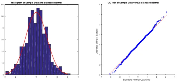
Figure 1.2: Histograms and normal probability plots for standardized ˆβ1 (upper

row) and ˆδ1,3 (lower row) with N =T = 80. Standardization used respectively the

[image:28.595.187.446.472.684.2]

(29)

1.1, which illustrates the convergence of βb and bδ respectively as N, T or both gets

larger.

Next we consider the asymptotic normality of ˆβ and ˆδ. We choose βb₁ and bδ₁_,₃ with

(N, T) = (80,80) as examples for illustration. For each simulation, we construct βb₁

and bδ₁_,₃, and standardize them according to the asymptotic results in Theorem 2

and Theorem 3 respectively. Figure 1.2 shows histograms and normal probability plots of the standardized estimators. They both show good fit for a standard normal distribution. It means that the asymptotic variance formulae in Theorem 2 and 3 are reliable for inference, and the way that we estimate any high dimensional covariance matrices mentioned in Section 1.4.1 helps in achieving an accurate estimation of the covariance matrices for βb andbδ. We actually get very similar good fits for the

non-zero components of ˜δ, showing the asymptotic normality in Theorem 4 is reliable as well. The results are omitted here to save space.

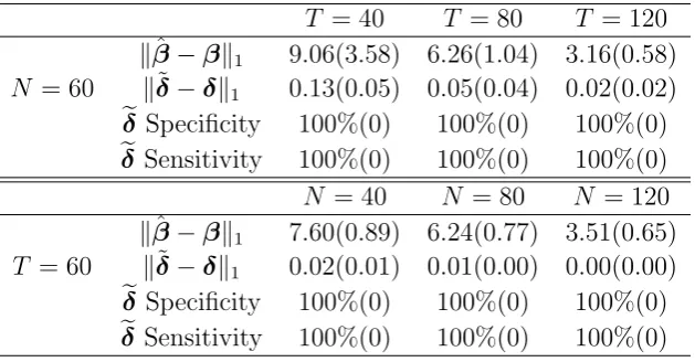
On top of asymptotic normality, ˜δ also enjoys sign consistency as shown in Theorem 4. We illustrate the selection consistency of ˜δin practice by calculating the specificity (i.e., proportion of correctly identified zeros) and the sensitivity (i.e., proportion of correctly identified non-zeros) ofeδ. Table 1.1 shows that at various combinations of

(N, T), the sensitivity and specificity are all 100%, showing perfect identifications of zeros and non-zeros. The table also shows the decreasing error forβb and eδ as N

orT increases.

T = 40 T = 80 T = 120 kβˆ −βk1 9.06(3.58) 6.26(1.04) 3.16(0.58)

N = 60 k˜δ−δk1 0.13(0.05) 0.05(0.04) 0.02(0.02)

e

δ Specificity 100%(0) 100%(0) 100%(0)

e

δ Sensitivity 100%(0) 100%(0) 100%(0) N = 40 N = 80 N = 120 kβˆ −βk1 7.60(0.89) 6.24(0.77) 3.51(0.65)

T = 60 k˜δ−δk1 0.02(0.01) 0.01(0.00) 0.00(0.00)

e

δ Specificity 100%(0) 100%(0) 100%(0)

e

[image:29.595.156.471.447.611.2]

δ Sensitivity 100%(0) 100%(0) 100%(0)

Table 1.1: Mean L1 error for βb and ˜δ. Standard deviations are shown in brackets.

Sensitivity and specificity ofeδ are also shown for various combinations ofT, N. The

values of bβ−β

1 are multiplied by 10 4_.

1.5.2

Cross-sectional dependence in the innovation

(30)

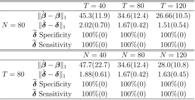
depen-matrix Σ_i,j = α|i−j| and α = 0.8. The results about the proposed estimators are shown in Table 1.2 when different combinations of sample size T and panel dimen-sion are used. First, the spatial weight matrix selection results are still perfect, as all values of eδ Specificity and Sensitivity are 100% for different T and N. Secondly,

the meanL1 errors forβb and ˜δ become significantly large than the simulation where

there is no cross=sectional dependence in the innovation process generation. How-ever, with the increase of sample size T or panel dimension N, the mean L1 errors

for βb and ˜δ decrease.

T = 40 T = 80 T = 120 kβˆ−βk1 45.3(11.9) 34.6(12.4) 26.66(10.5)

N = 80 kδ˜−δk1 2.02(0.70) 1.67(0.42) 1.51(0.54)

e

δ Specificity 100%(0) 100%(0) 100%(0)

e

δ Sensitivity 100%(0) 100%(0) 100%(0) N = 40 N = 80 N = 120 kβˆ−βk1 47.7(22.7) 34.6(12.4) 28.0(10.8)

T = 80 kδ˜−δk1 1.88(0.61) 1.67(0.42) 1.63(0.45)

e

δ Specificity 100%(0) 100%(0) 100%(0)

e

[image:30.595.155.473.224.388.2]

δ Sensitivity 100%(0) 100%(0) 100%(0)

Table 1.2: Mean L1 error for βb and ˜δ when innovation process contains

cross-sectional dependence. Standard deviations are shown in brackets. Sensitivity and specificity of eδ are also shown for various combinations of T, N. The values of

bβ−β

1 are multiplied by 10 4_.

1.5.3

Performance of BIC for choosing

p

To examiner the performance of the BIC defined in (1.8), we run our simulations 100 times for each particular (N, T) combination using the same setting as before, except that each time p is randomly generated from 1 to 7. With each simulation, we construct the positive selection rate (PSR) and the false discovery rate (FDR), defined as

PSR =

P100

j=1|s

∗

j ∩s0,j|

P100

j=1|s0,j|

, FDR =

P100

j=1|s

∗

j ∩sc0,j|

P100

j=1|s

∗ j|

,

where s0,j represents the index set for all δir that should be included in the model at the jth repetition. Since we do not set δir to be exactly 0 in this experiment, we have |s0,j| = pM = 3p, where p is in fact different for different j. The set s∗j is the index set for all bδ_ir estimated when p is estimated as p∗. Clearly, if p∗ ≤ p,

then |s∗

j ∩s0,j| =|s∗j| and |s ∗

(31)

other hand, if p∗ > p, then |s∗

j ∩s0,j| =|s0,j| and |s∗j ∩sc0,j| > 0, meaning we have included all that are in s0,j, but we have falsely “discovered” something outside of s0,j. Hence in a sense, PSR measures an average number of times where we do not underestimate p, while FDR measures an average number of times we overestimate p. Ideally, we want PSR=100% while FDR = 0%. These two measures are also used in Chen and Chen (2008) and Chen and Chen (2012) in different contexts.

T = 40 T = 50 T = 60 N = 50 PSR 100.00% 100.00% 98.00%

FDR 2.00% 0.00% 0.00%

N = 40 N = 50 N = 60 T = 50 PSR 98.00% 100.00% 100.00%

FDR 0.00% 0.00% 2.00%

Table 1.3: Positive selection rate (PSR) and false discovery rate (FDR) for the choice of pusing BIC defined in (1.8).

Table 1.3 shows the results. Our BIC definitely performs very well with PSR almost always equal 100% and FDR 0% in various (N, T) combinations.

1.6

Analysis of Stock Return Data

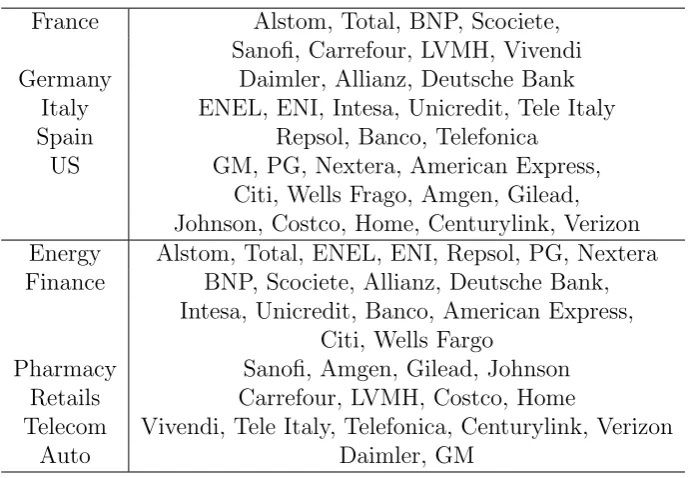
Spatial lag model has been widely applied to economic or geographic data, yet financial data is rarely analyzed using spatial econometrics tools. We illustrate the performance of our model using the daily log-returns of 32 important stocks shown in the following table in the Euro Stoxx 50 and S&P 500 in 2015. Our aim is to analyze the spatial interactions of these stocks and to see how different macroeconomic and financial indicators affect the dynamics of the returns.

(32)

France Alstom, Total, BNP, Scociete, Sanofi, Carrefour, LVMH, Vivendi Germany Daimler, Allianz, Deutsche Bank

Italy ENEL, ENI, Intesa, Unicredit, Tele Italy Spain Repsol, Banco, Telefonica

US GM, PG, Nextera, American Express, Citi, Wells Frago, Amgen, Gilead, Johnson, Costco, Home, Centurylink, Verizon Energy Alstom, Total, ENEL, ENI, Repsol, PG, Nextera Finance BNP, Scociete, Allianz, Deutsche Bank,

Intesa, Unicredit, Banco, American Express, Citi, Wells Fargo

Pharmacy Sanofi, Amgen, Gilead, Johnson Retails Carrefour, LVMH, Costco, Home

Telecom Vivendi, Tele Italy, Telefonica, Centurylink, Verizon

Auto Daimler, GM

To fill in this gap and generalize on their model, we include four types of spa-tial weight matrix specifications instead of only three matrices as in Arnold et al. (2013a). The first type is on the physical distance dij between city i and j where the headquarters of the stocks’ associated companies are built. As stock market is significantly affected by the local economy and, in spatial economy research, physi-cal distance is commonly used. In our case, three specified spatial weight matrices with elements 1/dij,1/d2_ij and 1/d3_ij are included for selection. The second to fourth types coincide with the three matrices specified in Arnold et al. (2013a). Namely, one contains the weight of stocks in Euro Stoxx 50 or S&P 500, and the remaining two having (i, j)th element equal to 1 if the corresponding stocks belong to the same industry or country respectively. This way, we have M = 6 specified spatial weight matrices for selection in our model. We have done row standardization on all of these six matrices.

[image:32.595.140.489.67.306.2]

As for the covariates Xt, we use the Fama-French three factors (excess return = market return - risk free rate, SMB = Small (market capitalization) Minus Big, HML = High (book-to-market ratio) Minus Low), national stock index (S&P 500, CAC40, DAX, IBEX or MIB) and the corresponding European or US industry index for each stock. Hence K = 5, and we are treating these as exogenous covariates, so we set Bt = Xt, the same as the covariates. Minimizing the BIC defined in (1.8) results in p= 1.

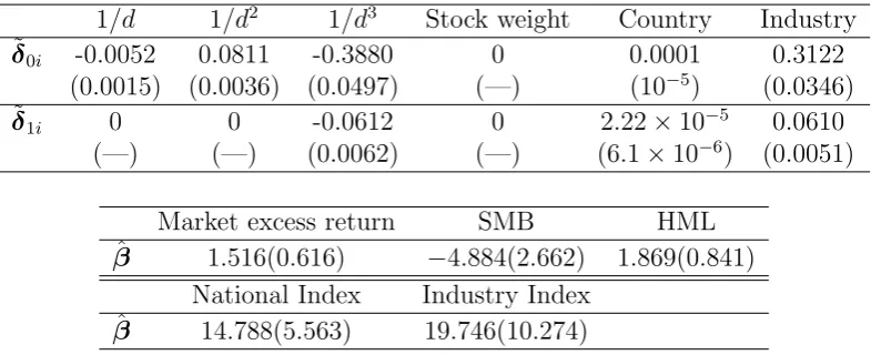
Table 1.4 shows the values of ˜δ. Clearly, stock weight in their respective market indices do not contribute to the two spatial weight matricesW0 and W1. However,

(33)

1/d 1/d2 1/d3 Stock weight Country Industry ˜

δ0i -0.0052 0.0811 -0.3880 0 0.0001 0.3122

(0.0015) (0.0036) (0.0497) (—) (10−5₎ _(0.0346)

˜

δ1i 0 0 -0.0612 0 2.22×10−5 0.0610

(—) (—) (0.0062) (—) (6.1×10−6₎ _(0.0051)

Market excess return SMB HML

ˆ

β 1.516(0.616) −4.884(2.662) 1.869(0.841) National Index Industry Index

ˆ

[image:33.595.116.509.69.229.2]

β 14.788(5.563) 19.746(10.274)

Table 1.4: The values of eδ and βb, where p = 1 and γ_T = 1.6438 are chosen by

minimizing the BIC defined in (1.8). Estimated standard deviations are in brackets. All values associate with βb are multiplied by 106.

chooses a distance 1/d, 1/d2 _{or 1/d}3 _{for the spatial weight matrix would fail, since}

it is clear that all three specified spatial weight matrices are significant and cannot be omitted for W0. Only the one for 1/d3 is significant to W1 though. In the

same table, we can see that all factors in Xt are at least marginally significant, with national and industry indices play a more important role practically than the Fama-French three factors.

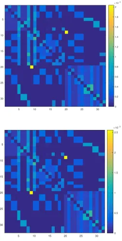
Figure 1.3 shows the heat map of the spatial weight matricesW0andW1. It is clear

that there are some block patterns in these matrices, which mainly represent stocks in the same country or industry. Meanwhile, they are related strongly with each other in general if they are all from Europe or US, with France and Italy showing strong connections. It is interesting to note that the ninth stock Daimler, and the twentieth stock GM, are related to each other (two bright yellow dots on both W0

and W1), although they belong to Germany and US auto-industry respectively.

Since Daimler owns part of GM by spin-offs, the relation itself is not surprising. However, it means that our method of taking linear combination of different specified spatial weight matrices can indeed reflect a general pattern of spatial interactions. In W1, we can also find some blocks for stocks in Germany and Spain.

1.7

Conclusion

(34)

individ-5 10 15 20 25 30 5

10

15

20

25

30

×10-3

0 0.2 0.4 0.6 0.8 1 1.2 1.4 1.6 1.8 2

5 10 15 20 25 30

5

10

15

20

25

30

×10-3

[image:34.595.188.441.129.627.2]

0 0.5 1 1.5 2 2.5

Figure 1.3: Upper: The estimate of W0. Lower: The estimate of W1. From 1 to

(35)

and the asymptotic normality results are built in the case when both the sample size T and panel dimension N go to infinity. Using instrument-like variables, the inconsistency from innate endogeneity in least square estimators can be fixed. Our model uses different linear combination of a set of specified spatial weight matrices for different spatial effects to avoid the misspecification. However, it is highly likely that some irrelevant spatial weight matrices are considered into the model, which may cause a new bias for the spatial weight matrix estimation. A further selection on spatial weight matrices included into our model is applied by adaptive LASSO proposed in Zou (2006), which can reflect which spatial weight matrices truly contribute which ones do not.

As for the prediction ability of our model, it is easy to have the predictive value by:

ˆ

y_t= (I −Wˆ0)−1( ˆµ+ ˆW1yt−1+· · ·+ ˆWpyt−p +Xtβˆ).

Same as the most of VAR (Vector AutoRegression) model, our model dose not have a good predictive ability when the panel dimension N is large. The estimated inverse matrix in the above predictive model do not perform well, which causes the predictive values inaccurate. However, the main goal of this Chapter is to construct the spatial weight matrix by high order spatial autoregression model and do a selection on the candidates of specified spatial weight matrices. We can leave the forecasting problem as a future work.

For the future study, first of all, the fixed M assumed in the proposed method can be extended to infinite M to reflect the practical reality that richness of a parametric model often deepens with sample size. Furthermore, it may be of interest to increase the efficiency of spatial weight matrix estimation. As known, adaptive LASSO is good in spatial weight matrices selection, however, it introduces some bias into the spatial weight matrix estimation as the sacrifice of sparseness. In Lam and Souza (2015c), adding a potentially sparse adjustment matrix for contemporaneous spatial effect is discussed, which can be extended to dynamic spatial model we proposed in this chapter. In the case of p is not large, quasi-maximum likelihood estimation can also be applied, especially when the instrument-like variable is not available. The last but not the least, we can still apply the proposed method but replace the L1 penalty by ridge regularization, which performs better in estimation but not in

(36)

1.8

Proof

1.8.1

Technical assumptions

Before the proof is provided, we present and explain more technical assumptions of the paper in this section. Most of these assumptions are extended from Lam and Souza (2015a).

R1. The column vectors vec(WT₀_i) in V0 are linearly independent to each other,

such that there exists a constant u > 0 with σ2

M(V0) ≥ u > 0 uniformly as

N → ∞, whereσi(A) is the ith largest singular value of a matrix A. Moreover, max1≤i≤MkW0ik1 ≤c <1 uniformly as N → ∞ for some constantc > 0.

R2. Writet=Σ1/2 ∗

t, whereΣ is the covariance matrix fort. Then the elements inΣ are all less thanσmax2 uniformly asN → ∞. Same for the variance of the

elements in Bt. We also assume kΣ1/2k∞ ≤ S < ∞ uniformly as N → ∞, with {∗

t,j}1≤j≤N being a martingale difference with respect to the filtration generated by σ(∗_t,₁, ..., ∗_t,j). The tail condition P(|Z| > v) ≤ D1exp(−D2vq)

is also satisfied by∗_t,j.

R3. All singular values of_E(XT_tBt) are uniformly larger thanN ufor some constant u >0, while the maximum singular value is also of orderN. Individual entries in the matrix _E(xtbTt) are uniformly bounded away from infinity.

R4. For the same constant a, we have for each N

max

1≤i≤N N

X

j=1

E(

X

q≥0

bt,ixTt−q,j)

max

, max

1≤j≤N N

X

i=1

E(

X

q≥0

bt,ixTt−q,j)

max

≤CbxNa

where Cbx > 0 is a constant and bt,i, xt,j are the column vectors for the ith row ofBt and jth row ofXt respectively. At the same time, assume also that

E(Xt⊗Btζ) has all singular values of order N1+a.

R5. Assume 0 < b < 1. For fixed = 1, . . . , K, the eigenvalues of N−bvar(Bt,k) and var(T) are uniformly bounded away from 0 and infinity, and respectively dominates the singular values of the sum of N−bcov(Bt+τ,k,Bt,k) over τ 6= 0 and the sum of _E(tTt+τ) over τ 6= 0. Also, for eachi = 1, . . . , N, we assume that

X

τ

σi N−bcov(Bt+τ,k,Bt,k)

<∞, X τ

σi _E(tt+τ)

(37)

R6. Define λT =cT−1/2log1/2(T ∨N) for some constant c >0. The tuning param-eter γT is such that γT =CλT for some constant C > 0.

R7. In all the assumptions above, we assume that as N, T → ∞, λTN1−a =o(1), N−a+b−1/w_log−1_(T_∨_N_{) =}_{o(1), log(T}_∨_N_)N1/w−b ₌_{o(1) and}_Nb−a₌_{o(T λ}

T). Assumption R1 essentially requires that each specificationW0i is different from one another to a certain extent. This is intuitive, since if W0i and W0l are too similar to each other, the coefficients δji and δjl are not well defined, and this will have a negative impact on the performance of our estimators.

The assumptions on Σ in R2 is mainly for the convenience of proofs, while the martingale difference assumption for t is a relaxation to independence.

Assumptions R3 and R4 are closely related. They paint a picture of how the ex-ogenous variables in Bt are correlated with Xt−q. Assumption R3 essentially says that the covariance between a variable in Bt and one in Xt is finite uniformly as N → ∞. Then for k = 1, . . . , K, considering the kth diagonal entry of _E(XT_tBt) is PN

j=1E(Xt,jkBt,jk) with each E(Xt,jkBt,jk) being finite, it is indeed reasonable to

assume that each diagonal entry in the matrix is of order N. This assumption is needed for the estimator β=β(δ) to be well-defined.

Assumption R4 essentially describes how each row of variables in Bt are correlated with different rows of variables inXt. With this, we can actually derive easily that k_E(Xt⊗Btζ)k1 has order at most N1+a. Hence the assumption of having all the

singular values of _E(Xt⊗Btζ) of orderN1+a is reasonable.

Assumption R5 assumes a rate for the singular values of var(Bt,k) essentially, which is important in certain asymptotic normality results. The rateNb, possibly differing fromNa, is reasonable as well since the way that Bt and Xt are correlated do not directly indicate how the variables inBt itself are correlated, unless of course when

Bt =XtwhereXtitself is exogenous, in which casea=b. The variance-covariance matrix being dominating the lag τ auto-covariances is for the ease of presentation of rates of convergence in the asymptotic normality results in this chapter.

1.8.2

Proof of theorems

The followings are Lemma 1 and 2 of Lam and Souza (2015a) respectively.

Lemma 1. For a zero mean time series processxt =f(F)with dependence measure θx

t,d,j defined in Section 1.3, assumeΘxm,a≤Cm

(38)

P(|1/T T

X

t=1

xt,j|> v)≤ C1T

w(1/2−α˜)

(T v)w +C2exp(−C3T

˜

β v2),

where α˜ =α∧(1/2−1/w), and β˜= (3 + 2 ˜αw)/(1 +w).

Furthermore, assume another zero mean time series process zt (can be the same

process xt) with both Θxm,2w, Θzm,2w ≤Cm

−α_{, as in Assumption M3. Then provided}

maxjkxtjk2w, maxjkztjk2w ≤c0 ≤ ∞where c0 is a constant, the above Nagaev-type

inequality holds for the product process {xtjztl−E(xtjztl)}.

Lemma 2. For any N ×N matrix H = (h1, . . . , hN)T and any N ×K matrix M,

define

VH =      

IK⊗h1

.. .

IK⊗hN

      .

Then we have

HM = (IN ⊗vecT(M))VH.

We first present an Theorem 5 which states that a set M is such that P(M)→ 1 as T, N → ∞, and our estimators enjoy nice properties on M. This theorem is in fact exactly the same as Theorem S.1 of Lam and Souza (2015a).

Denote Bt,ij and Xt,ij the (i, j) entry of Bt and Xt respectively, and define M = ∩7

i=1Ai, where

A1 =

(

max

1≤i,k≤N1≤j,l≤Kmax |T −1

T

X

t=1

[Bt,ijXt,kl−_E(Bt,ijXt,kl)]|< λT

)

,

A2 =

(

max

1≤i,k≤N1max≤j≤K|T −1

T

X

t=1

Bt,ijt,k|< λT

)

,

A3 =

(

max

1≤k≤K|T −1 T X t=1 N X s=1

Bt,skt,s|< λTN1/2+1/2w

)

,

A4 =

max

1≤i≤N1max≤j≤K| ¯

B.,ij−_E(Bt,ij)|< λT

,

A5 =

max

1≤j≤N|¯.,j|< λT

,

A6 =

max

1≤i≤N1max≤j≤K| ¯

X.,ij|< λT

,

A7 =

(

max

1≤k≤K| N

X

s=1

¯

B·,sk¯.,s|<21/2λTN1/2log1/2(T ∨N)S(max

i.j |E(Bt,ij)|+λT)

)

(39)

Theorem 5. Let Assumptions M1-M4 in Section 1.3.1 and R1-R7 in Section 1.8.1

hold. Suppose α ≥ 1/2−1/w in Assumption M3, and for the application of the

Nagaev-type inequality in Lemma 1 for the processes defined in A1 to A7, suppose

the constants C1, C2 and C3 are the same. Then with c ≥

p

3/C3 where c is the

constant defined in λT =cT−1/2log1/2(T ∨N), we have

P(M)≥1−8C1K2(C3/3)w/2

N2

Tw/2−1_logw/2_(T _∨_N₎−

8C2K2N2

T3_∨_N3 −

2K T ∨N.

It approaches 1 if we assume further that N =o(Tw/4−1/2_logw/4_(T₎₎_.

Proof of Theorem 1

From (1.4) and that

yv₀ = M

X

i=1

δ0iW⊗0iy v 0+ p X j=1 _XM i=1

δjiW⊗0i

yv_j +Xβ+v+1T ⊗µ =IT N −

M

X

i=1

δ0iW⊗0i

−1_Xp

j=1

_XM

i=1

δjiW⊗0i

yv_j +Xβ+v +1T ⊗µ

,

it is easy to get, sinceBvT(1T ⊗µ) =0, that

β(δ)−β= (XTBvBvTX)−1XTBvBvTv.

Moreover,

b

β =β(ˆδ)

= (XTBvBvTX)−1XTBvBvThIT N − M

X

i=1

ˆ δ0iW⊗0i

yv₀− p X j=1 _XM i=1 ˆ δjiW⊗0i

yv_ji

= (XTBvBvTX)−1XTBvBvT

h

IT N − M

X

i=1

δ0iW⊗0i

yv₀− p

X

j=1

_XM

i=1

δjiW⊗₀_i

yv_j

+ M

X

i=1

(δ0i−δˆ0i)W⊗0iyv0 +

p

X

j=1

_XM

i=1

(δji−δˆji)W⊗0i

yv_ji

=β(δ) + (XTBvBvTX)−1XTBvBvT

·h M

X

i=1

(δ0i−δˆ0i)W⊗0iy v 0 + p X j=1 _XM i=1

(δji−δˆji)W⊗0i

(40)

Using the above, we can decompose

ˆ

β−β=I0+I1+I2+I3+I4+I5, where

I0 = (E(XTtBt)E(BTtXt))−1(E(XTtBt)E(BTtXt)−T−2XTBvBvTX)( ˆβ−β), I1 = (E(XTtBt)E(BTtXt))−1T−2XTBvBvTv,

I2 = (E(XTtBt)E(BtTXt))−1T−2XTBvBvT( M

X

i=1

(δ0i−ˆδ0i)W⊗0i)Π ⊗

Xβ,

X

i=1

v,

X

i=1

( p

X

j=1

( M

X

i=1

δjiW⊗0i)y v j),

I5 = (E(XTtBt)E(BtTXt))−1T−2XTBvBvT( p

X

j=1

( M

X

i=1

(δji−δˆji)W⊗0iy v j)),

with Π⊗ = (IT N −P_iM₌₁δ0iW⊗0i)

−1_{. We need to find the rate of convergence of} _I 0

I1,I2, I3, I4 and I5.

To this end, using Assumption R3 in Section 1.8.1,

k_E(XT_tBt)E(BTtXt)−1k1 ≤

K1/2

λmin(E(XTtBt)E(BTtXt)) ≤ K

1/2

N2_u2.

Define U = IN ⊗T−1PT_t₌₁vec(Bt−B¯)vecT(Xt) and U0 = IN ⊗E(btxTt), then we can write T−1XTBv =VT_I_NU VIN and E(X

T

tBt) =V T

INU0VIN. Also, denote

(41)

jth row of Π. Then on M,

kI0k1

≤ k(_E(XT_tBt)E(BtTXt))−1k1k((E(XTtBt)E(BTtXt))−T−2XTBvBvTX)( ˆβ−β)k1

≤ K

1/2

N2_u2

kVT_I_N(U0−U)TVINV

T

INU0k1

+kVT_I_NUTVINV

T

IN(U0 −U)k1

kVIN( ˆβ−β)k1

≤ K

1/2

N2_u2

KkU0 −Ukmax·N ·KkU0kmax

+ (KkVT_I

N(U −U0)

T_V

INkmax+KkV

T

INU

T

0VINkmax)·KkU0−Ukmax

·Nkβˆ−βk1

≤K1/2(2λTσbx(1 +µb,max+λT) +λT2(1 +µb,max+λT)2)kβˆ−βk1

=O(λTkβˆ −βk1),

where µb,max=

E(b_t)

max. At the same time, onM,

kI1k1 ≤

K1/2 N2_u2kT

−1

XTBvk1kT−1BvTvk1

≤ K

1/2

N2_u2kV

T

IN(U −U0)VIN +V

T

INU

T

0VINk1

·(KλTN1/2+1/2w + √

2KλTN1/2log(T ∨N)S(µb,max+λT)) ≤ K

1/2

N2_u2N(λT(1 +µb,max+λT) +σbx)

·(KλTN1/2+1/2w + √

2KλTN1/2log(T ∨N)S(µb,max+λT)) =O(λTN−1/2+1/2w).

(42)

then onM,

kI2k1 ≤

K1/2 N2_u2kT

−1_XT

Bvk1kT−1

T

X

t=1

(Bt−B¯)T(W0−Wˆ 0)ΠXtk1kβk1

≤ K

1/2

N2_u2O(N)

K· max

1≤r≤K N X j=1

(Wc₀_,j−Wˆ c₀_,j)TT−1 T

X

t=1

(Bt,r−B¯.,r)XTt,rπj

≤O(N−1)( N

X

j=1

(λT(1 +µb,max+λT) +σbx)kWc0,j −Wˆ c

0,jk1kπjk1)

≤O(N−1)(Nkδ0−δˆ0k1) = O(kδ0−ˆδ0k1).

Similarly, onM,

kI3k1 ≤

K1/2

N2_u2kT

−1_XT_Bv_k

1kT−1

T

X

t=1

(Bt−B¯)T(W0 −Wˆ 0)Πtk1

≤ K

1/2

N2_u2O(N)

K max 1≤r≤K N X j=1

(Wc₀_,j−Wˆ c₀_,j)TT−1 T

X

t=1

(Bt,r−B¯.,r)Tt

πj

≤O(N−1)·O(N λT max

1≤j≤N

π_j

1₁max_≤j≤N

Wc₀_,j−Wc

c

0,j

1) =O(λT

δ₀−bδ₀

1).

For bounding I₄ 1 and I₅

1, recall that from Section 1.3.1, we can expressyt as

y_t=Φ−1(L)Π(µ+Xtβ+t) =

X

q≥0

ΨqΠ(µ+Xt−qβ+t−q), (1.9)

where Ψq is N ×N such that

P

q≥0

Ψ_q

_∞ <∞ because of stationarity. Then we

can decompose

kI4k1 ≤

K1/2 N2_u2kT

−1_XT_Bv_k

1 · T −1 T X t=1

(Bt−B¯)T(W0−Wˆ 0)Π

p

X

j=1

WjΦ−1(L)Π(Xt−jβ+t−j)

1

=O(N−1(kI41k1+kI42k1)), where

kI41k1 =

T −1 T X t=1

p

X

j=1

WjΦ−1(L)ΠXt−jβ

1, I₄₂ 1 = T −1 T X t=1

p

X

j=1

WjΦ−1(L)Πt−j

(43)

On M, we have

I41

1 ≤₁max_≤j≤p₁_≤r,k≤Kmax pK 2 β 1 · X q≥0 n

T−1 T

X

t=1

(Bt,r−B¯·,r)T(W0−Wc₀)ΠW_jΨ_qΠXt−q−j,k

o

=O(N σbx

W0−Wc0

_∞ Wj _∞ Π 2 ∞ X q≥0 Ψq _∞)

=O(Nδ0 −bδ₀

1),

where the second line is by Assumption R4. At the same time onM,

I₄₂ 1 ≤ max

1≤j≤p1max≤r≤KpK

X q≥0 n

T−1 T

X

t=1

(Bt,r−B¯·,r)T(W0−Wc₀)ΠW_jΨ_qΠt−q−j

o

=O(N λT

W₀−Wc₀ _∞ W_j _∞ Π 2 ∞ X q≥0 Ψ_q _∞)

=O(N λT

δ₀−bδ₀

1),

where the second line follows from the rate onA2. These imply that on M,

I₄

1 =O(

δ₀−bδ₀

1).

To bound I₅

1, we can decompose

kI5k1

≤ K

1/2

N2_u2kT

−1_XT_Bv_k

1 T −1 T X t=1

(Bt−B¯)T p

X

j=1

(Wj−Wˆ j)Φ−1(L)Π(Xt−jβ+t−j)

1

(44)

Spatial modelling and volatility matrix estimation in high dimension statistics with financial applications