Algorithmic learning from financial predictions

(1)

Algorithmic Learning from

Financial Predictions

Pongphat Taptagaporn

A thesis submitted to the Department of Mathematics of the London School of Economics for the

(2)

“The advantage scientists bring into the game is not their mathematical or computational skills than their ability to think scientifically. They are less likely to accept an apparent winning strategy that might be a mere statistical fluke.”

(3)

Declaration

I certify that the thesis I have presented for examination for the PhD degree

of the London School of Economics and Political Science is solely my own

work other than where I have clearly indicated that it is the work of others (in which case the extent of any work carried out jointly by me and any other

person is clearly identified in it).

The copyright of this thesis rests with the author. Quotation from it is

permitted, provided that full acknowledgement is made. This thesis may not be reproduced without my prior written consent.

I warrant that this authorisation does not, to the best of my belief, infringe the rights of any third party.

Statement of conjoint work:

I confirm that some of the content of Chapter 4 of this thesis was presented as co-authored work with my supervisor, Dr Tugkan Batu, at the 27th

Interna-tional Conference on Algorithmic Learning Theory, published in the Lecture

Notes in Artificial Intelligence, Volume 9925, pp 288-302, Springer 2016. Ci-tation [BT16].

The contents of Chapter 5 of this thesis is also currently being reviewed for conference publication as co-authored work with Dr Tugkan Batu.

Cita-tion [BT17].

(4)

Abstract

We study how financial predictions can be used in learning algorithms for

problems such as portfolio selection and derivatives pricing, from the

perspec-tive of minimizing regret; the worst-case loss (across all possible price paths) against some optimal benchmark model with superior information. Unlike

most studies in financial mathematics, we do not make any underlying

as-sumptions beyond the existence of such predictions, so our results are robust in the model-free sense.

This thesis consists of three main ideas:

1. Study a portfolio selection model that competes with an optimal static trading strategy (the best fixed strategy in hindsight) using predictions

of the optimal portfolio allocation.

2. Study a portfolio selection model that competes (in probability) with an

optimal dynamic trading strategy (the best greedy strategy in hindsight) using price predictions of each asset in the portfolio.

3. Derive robust derivative pricing bounds for vanilla options and various

exotic derivatives based on price predictions of the underlying asset(s).

This work is focused on the mathematical analysis of these models, using

(5)

Acknowledgement

First and foremost I would like to sincerely thank Dr Tugkan Batu for the

supervision throughout my PhD program. His guidance and constant support

have been invaluable. I would also like to thank my second supervisor, Prof Martin Anthony, for his wisdom and feedback on my research. I am grateful

to the examiners, Dr Yuri Kalnishkan and Dr Varun Kanade, for their useful

comments on this thesis.

I would like to thank everyone in the Mathematics department at the LSE for providing a pleasant and stimulating atmosphere to carry out academic

research. It has been enjoyable and satisfying.

Finally, I gratefully acknowledge funding from the LSE’s PhD scholarship

that has given me the opportunity to explore interesting research, and funding

from the Mathematics department for attending overseas conferences, among other things.

(6)

Chapter 1

Introduction

Much of the studies in financial mathematics can be broadly categorised into

theQandPworlds. TheQworld is in the realms of derivative pricing (calibrat-ing the fair price of securities based on market variables), while the P world studies portfolio management problems (estimating the statistically derived

probability distribution of asset prices and constructing efficient portfolios). In both cases, much of the work often rely on assumptions of the underlying

market dynamics. In particular, these results typically make statements of the

form:

“If variable X has dynamics Y, then ....”

Perhaps the most famous examples are the Merton portfolio [Mer71] and Black-Scholes option pricing [BS73], whose results depend on the

underly-ing asset price evolvunderly-ing as Geometric Brownian Motion (GBM), among other things. While these have been widely adopted by practitioners and received

much success from industry, there has also been much criticism about the

in-consistencies of these underlying assumptions to the observed behaviour from the financial market. For example, the existence of volatility smile in the

foreign exchange options market [Hul06].

This work aims to provide robust (model-free) approach to these problems

in the Q and P worlds. In particular, we will provide algorithms for portfo-lio selection and derivatives pricing that will work regardless of how market

(10)

dynamics behave. Instead of making assumptions on the underlying market dynamics, we assume the existence of predictions of various parameters to

assist in the decision-making process, for example, predictions on the future

asset price (often referred to as “alpha” in the financial industry) or optimal portfolio distribution.

Without making any assumptions on the underlying market dynamics, it

is impossible to say anything meaningful about the average-case performance

of these algorithms. Therefore, the performance of these models are analyzed relative to some optimal benchmark adversary (typically with access to

supe-rior information). The performance of such algorithms (relative to the optimal

benchmark) would then depend on the quality of the predictions received.

1.1

Literature Review

A new field emerged in the 1990’s that uses game theory and machine

learn-ing to design portfolio selection models that performs competitively without making any conjecture on the future. The first known paper in this field by

Thomas Cover [Cov91] introduced a portfolio model that makes decision on

the portfolio distribution among assets purely based on current and past in-formation; it does not assume any prediction mechanism. Most interestingly,

he was able to prove a worst-case performance guarantee (across all possible

price paths), as compared to the wealth of the best fixed (static) strategy in hindsight, without making any assumption on how the price must evolve. In

particular, it was shown that a regret of

max

xT

logS∗_T −log ˆST

=O(logT)

is attainable whereS_T∗ is the wealth obtained from the best constant-rebalanced portfolio (CRP) in hindsight, and ˆST is the wealth obtained from the

compet-ing portfolio model (Cover’s universal portfolio), over T discrete time steps. The maximum difference in log-wealth is taken over all possible price paths

xT. Note that a CRP is defined as an investment strategy with the

restric-tion that it must maintain a fixed proporrestric-tion of wealth in each of the assets throughout all time steps, performing any required rebalancing as to maintain

(11)

of such strategy that maximizes wealth over allT time steps.

The general idea of Cover’s algorithm is to take a weighted combination of portfolios according to some prior distribution (hence “universal”), and run

them independently, performing any required rebalancing as to maintain the

CRP assumption across each of these constituent portfolios. The key to prov-ing the regret bound is that by usprov-ing a weighted combination of portfolios, the

algorithm would have picked a sufficient number of sample portfolios “nearby”

the best CRP, which will then perform similarly. The bad performing port-folios would then die off and the better performing ones would dominate,

resulting in a wealth that is bounded against the best CRP.

Since then, there has been much follow up work and extensions to Cover’s

original portfolio model. For example, some research [CO96, BS10, BS11,

KACS15] extended Cover’s universal portfolio to compete against a stronger benchmark using a concept of “side information”. This is where the adversary

reveals a side information (say, an integer between 1 and y) and the CRP

restriction is applied on each state separately. In particular, there is now y

different CRPs that may be used, depending on the side information in that

particular time step. The benchmark in this case is the best set ofyCRP’s that

achieves the highest wealth, given the observed sequence of side information. However, the regret bound of this model assumes that y is finite and does

not grow with T, meaning that sublinear regret bound does not hold if the benchmark model uses a different portfolio in every time step, i.e., the side

information never repeats.

One possible extension when studying portfolio models is to include the

presence of market friction in the form of transaction cost, to mimic the

be-haviour of modern order-driven market. This concept was introduced in the context of universal portfolios by Blum and Kalai [BK99], where they charged

a fixed percentage of commission as a proportion of the traded volume.

Hazan et al. [HK09] showed an alternative regret bound for Cover’s

univer-sal portfolio of O(logQ), whereQis the quadratic variation of the underlying assets (similar to the notion of volatility). However, one can realistically

ex-pect Qto grow with T, hence still has the dependence onT nevertheless.

Recall that Cover’s original portfolio model (as well as most research in

this field) assumes trading in discrete time steps. Freund [Fre09] demonstrated

(12)

the extension of another similar portfolio selection algorithm from Chaudhuri et al. [CFH09] in the continuous-time setting by modelling the stochastic price

process as an Itˆo process.

More recent efforts [CYL+12, RS13] incorporated predictions into online

learning problems. These work look at the more general case of convex loss functions, as compared to the log-wealth in the portfolio setting. Some other

variants of the universal portfolio can be found in [AH06, AHKS06, Cov96,

GW12, HAK07, KW99, OC96, SL05]. Most of these models are based on the idea of taking a weighted combination of CRPs over the set of all possible

portfolio vectors, as in the case of Cover’s universal portfolio. Therefore, it

was natural in these settings to then compare the wealth to the best fixed strategy in hindsight.

In 2006, DeMarzo et al. [DKM06] showed that the regret of portfolio selec-tion algorithms naturally give rise to an upper bound for opselec-tions price in the

model-free sense, by replicating the payoff of an option by the returns of the

best performing asset in hindsight. However, their bound still depends on the volatility of the underlying asset (through the quadratic variation Q), much

like in the Black–Scholes framework. In particular, they showed

C(K, T)≤Θ(pQ),

whereC(K, T) denotes the price of a call option (with strikeK at expiryT),

without making any additional assumptions on the underlying price process.

Follow up work from Gofer et al. [GM11a, GM11b, Gof14] extended this

result to price various exotic derivatives in the model-free sense, and Abernethy et al. [AFW12, ABFW13] showed that this option price bound converges to

that of Black-Scholes in the limit; as each time step increment→0, analogous to the continuous time setting).

1.2

Structure of the Thesis

First we will introduce the required notations and preliminary background in Chapter 2 that will be used throughout the thesis. Thereafter, this thesis

(13)

Chapter 3: Static Trading Strategy

Extend the results of Cover’s universal portfolio algorithm to account for transaction cost in the setting with multiple side information. We prove that

logarithmic regret against the best CRP with side information is attainable,

and provide an efficient approximation algorithm to compute such portfolio. We also examine the improvements that can be achieved by introducing the

notion of predictions of the optimal portfolio distribution.

Chapter 4: Dynamic Trading Strategy

We look beyond the restriction of the CRP from Chapter 3 to design a

portfolio selection algorithm that competes with a stronger benchmark, the

best greedy portfolio, in the stochastic setting. To do this, we make use of price predictions and prove that small expected regret (and variance of regret)

is attainable subject to the quality of such predictions. We also study the

case of incorporating transaction cost, and show that sub-linear regret is not attainable in this setting with non-zero transaction costs. The computation

of these portfolios will be shown to reduce to a linear program.

Chapter 5: Derivatives Pricing

Traditional option pricing model such as Black-Scholes assume that the

underlying asset follows a GBM. Alternatively, we derive a robust upper bound

on options price (that does not make any assumption on the underlying asset price process) using the expected regret bound from the predictive trading

strategy from Chapter 4. We first show a bound for pricing vanilla options,

then extend this to a number popular exotic derivatives.

(14)

(15)

Chapter 2

Preliminaries

This chapter will provide the preliminary definitions and ideas that will be

used throughout the thesis.

Consider the scenario where we have massets available for trading over T

discrete time steps. Define

xt= (xt(1),· · · , xt(m))∈Rm+

as a vector of price relatives (also known elsewhere as “returns vector”) at time stept, that is,xt(i) is the ratio of the true market price of assetiat time

tand timet−1. For example, if asset idid not change in price at timetthen

xt(i) = 1. This will be defined for 1 ≤t ≤T ∈ N, and use xt to denote the

price path up to timet,

xt:= (x1,· · · , xt).

Define a portfolio vector at timet as

bt= (bt(1),· · · , bt(m))∈ B={bt∈Rm+ :

m

X

i=1

bt(i) = 1}

where bt(i) is the proportion of the portfolio’s total wealth allocated to asset

i at time t. From time step t−1 to t, if we invest using portfolio bt in our

trading strategy then our wealth will change by a factor of

bt·xt,

(16)

i.e., the dot product of the twom-dimensional vectors, representing the change in value of the portfolio. OverT time steps, a trading strategy is specified by

the sequence of portfolio vectors

bT := (b1,· · · , bT)

and the total wealth becomes1

ST(bT) = T

Y

t=1 btxt.

Broadly speaking, ST is the product of the wealth change across all time

steps t ∈ [T]. Note that ST has hidden dependency on xT; we omit this

for notational convenience. Typically we may need to re-distribute wealth

between assets as to obtain the chosen portfolio vector for the next time step. We will call this re-distribution of wealth process “re-balancing”.

Similarly, for the trading strategies specified by (ˆb1, . . . ,ˆbT) and (b∗1, . . . , b∗T),

we will use ˆST and ST∗, respectively, to denote the wealth generated by the

corresponding portfolios.

A constant-rebalanced portfolio (CRP) is defined as the subset of bT with

the additional constraint that the portfolio vector is the same throughout every time step, that is,

b1 =· · ·=bT.

Although the portfolio model investigated here has the restriction that all the

wealth must be invested in one of themassets (imposed by the condition that

all of the individual asset wealths must sum up to one), this can be extended to a portfolio of m+ 1 assets where the first m assets are as before, and the

last one represents cash. Therefore, the returns xt now has m+ 1 dimension

where the last element could represent risk-free interest rate (from the change in value of the riskless asset), analogous to much of the work in financial

mathematics.

1_{The notations}_b

txtis used as a short-hand for vector dot product, and we may

(17)

2.1

Robust Performance Metric

There are a number of methods that have been used to measure performance

of portfolio selection models in literature, most commonly wealth, or some risk-adjusted notion of wealth. For example, modern portfolio theory [Mar52]

gives a framework to optimize the mean-variance of a portfolio.

Recall that our models do not make any assumption on the price movement

of the assets. Of course, with no additional assumption we cannot have any

guarantees regarding the future wealth. For example, if the price of all of the assets at a particular time decreases by 10%, our wealth will necessary

decrease by 10%, regardless of the portfolio distribution.

Therefore, we can only compare the wealth obtained by the portfolio as

compared to that of another portfolio. A common metric that has been used for this purpose is calledregret.

To understand the notion of regret, first assume that we know the wealth

ST (overT time steps) of our portfolio model and the wealthS∗T of the

bench-mark model (typically representing some notion of optimality). We wish to

evaluate the growth-rate of wealth, denoted byWT, such that ST =eWT, and

similarlyW_T∗ such thatS_T∗ =eWT∗. The worst-case difference (over all possible

price paths) between these exponential growth is called regret, namely

R:= max

xT (W

∗

T −WT) = max xT (logS

∗

T −logST).

This can also be viewed as the worst-case guarantee of the difference between

the logarithmic wealth factors of the benchmark model and the competing portfolio model. Suppose now that we do not know the exact values of ST

and S_T∗, but may be able to derive some bounds on them. The problem of minimizing R is known as regret minimization. Intuitively, a smaller regret bound implies that our model is closer to the benchmark model (in the

worst-case), thus closer to some notion of optimality.

Furthermore, to put the wealth ratio in context, we are generally interested

in the exponential growth rate per time step. This can be written as

R

T =

1

T maxxT (logS

∗

T −logST).

(18)

We say that the portfolio model has sublinear regret if this value is o(1) in

T, or equivalently, R = o(T). Intuitively, this means that the exponential

growth rate of wealth of the competing portfolio model converges to that of

the benchmark model, as the number of time steps grow large, T → ∞.

For probabilistic portfolio selection models where the trading strategy de-pends on some random choices (for example, random predictions), the regret

also becomes probabilistic. Then it seems natural to study the statistical

properties of the regret such as expected regret

E[R] :=E

max

xT (logS

∗

T −logST)

,

and the variance of regret

Var[R] := Var

max

xT (logS

∗

T −logST)

.

Academic studies in another related problem, the multi-armed bandit [BC12],

had also considered the notion of pseudo-regret,

¯

R:= max

xT E[logS

∗

T −logST],

While the notion of pseudo-regret is weaker than the expected regret with ¯

R≤E[R], bounds on the pseudo-regret imply bounds on the expected regret.

Much of the studies in online learning revolves around proving bounds for

the regret (or its various properties), although often differ in context.

2.2

Transaction Cost

Any realistic trading strategy would have to consider the effect of transaction costs on its profitability. As seen across most financial exchanges, market

makers, and brokers worldwide, the buying price of an asset is generally higher

than its selling price due to bid-ask spread.

The concept of transaction costs was first introduced into the study of

(19)

the sale, of assets. This is equivalent to charging commission on the purchase and sale of assets equally (as in modern limit-order markets), as the wealth

from any asset we sold will have to be used to purchase another asset (whether

it be kept in riskless cash, or another risky asset). We will use the same model here, though the choice of model doesn’t significantly affect our results.

Given portfolio vectors bt−1, bt ∈ B and returns vector xt−1, we want to

re-balance from the vector

b0_t−1 :=bt−1·xt−1∈Rm

to

bt∈ B ⊂Rm.

Given a transaction cost factor

c∈[0,1]

indicating the proportion of cost to be paid from the value of assets pur-chased, the proportion of wealth retained after rebalancing can be expressed

recursively as

θ:=θ(bt−1, bt, xt−1) = 1−c

X

i:βi>0

βi,

where

βi =θbt(i)−bt−1(i)·xt−1(i) =θbt(i)−b0t−1(i)

indicates the quantity of assetithat needs to be bought or sold, depending on

its sign. Intuitively, θ represents the proportion of the total wealth left after

rebalancing. In the worst case, the market value of b0 is at least 1−c of the market value ofbafter rebalancing. In particular, rebalancing a portfolio will

always retain at least 1−c proportion of its wealth. Note that c = 0 means that no transaction cost is charges and hence can be ignored.

We denote byθ(bt−1, bt, xt−1) the multiplicative factor of decrease in wealth

due to rebalancing from portfoliobt−1 (after observing the price change xt−1)

to portfolio bt. Then, we can define the wealth of a portfolio model (with

transaction cost) as

ST = T

Y

t=1

btxtθ(bt−1, bt, xt−1).

(20)

As a convention, we assume that there are no transaction costs associated with the initial positioning before the first time step: that is, b0 := b1, x0 =

(1, . . . ,1), and, thus,θ(b0, b1, x0) = 1.

Broadly speaking, ST is the product of the wealth change across all time

steps t ∈[T], where, at each step, we first pay a factor of θ(bt−1, bt, xt−1) in

transaction cost for re-balancing bt−1 tobt, and then experience a changebtxt

in wealth, once the price change is observed.

The transaction cost factorθcan be computed efficiently using either

ran-dom sampling or a linear program. These will be demonstrated as part of the

(21)

(22)

Chapter 3

Static Trading Strategy

In this chapter, we present an extension of Cover’s universal portfolio,

incor-porating the presence of transaction costs [BK99] in the setting with multiple discrete side information states [CO96]. We explore the case where we have a

prediction mechanism that is able to indicate approximately the best portfolio

distribution in some future time steps, and show that we are able to derive a portfolio selection algorithm that is competitive with the best static trading

strategy.

First we define the static trading strategy that will be used as the

bench-mark model. Recall that a constant-rebalanced portfolio (CRP) is an

invest-ment strategy where at every time step invest its wealth according to some portfolio distribution, say b. Over T time steps, the wealth achieved by the

CRP strategy then becomes

ST(b) = T

Y

t=1 bxt,

a special case of the (unrestricted) general strategy. We denote the best CRP

in hindsight (over T time steps) by the best portfolio distribution b∗ that maximizes precisely this wealth above. Formally,

b∗ = arg max

(23)

and denote the corresponding wealth of b∗ by

S_T∗ = max

b∈B ST(b).

3.1

Cover’s Universal Portfolio

Now we will formally describe Cover’s universal portfolio [Cov91]. Let µ be

a prior (initial) distribution function over the space B of m assets with the standard condition that

Z

B

dµ(b) = 1,

forb∈ B. Aµ-weighted universal portfolio is, roughly speaking, a (measure-theoretic) weighted combination of many different CRPs, with the initial

weighting rule according to the continuous prior distribution µ. Hence, the

measure of wealth invested in the CRP denoted bybisµ(b), and so the wealth due to b up to time t−1 is St−1(b)µ(b), yielding a total wealth (across the

whole spectrum of CRPs) of

Z

B

St−1(b)dµ(b).

In Cover’s definition of universal portfolio, the measure of each CRP are weighted by the amount of wealth they have historically generated. This

is equivalent to picking many CRP’s initially according to prior distribution

µ, then letting them run independently for the entire game (from t = 1 to

T). Conceptually, no re-balancing occurs across different CRP’s, but they are

each re-balanced independently of each other. Taking an integral over the continuous space of all portfolio vectors B, we get the wealth distribution for the universal portfolio,

Z

B

bSt−1(b)dµ(b).

Dividing this by the total amount of wealth currently available at time step

t−1 (so that the non-negative weights in the portfolio vector sums to 1), we get Cover’s universal portfolio.

(24)

Definition 1 ([Cov91]) The µ-weighted universal portfolio at time t is

ˆ

bt=

R

BbSt−1(b)dµ(b)

R

BSt−1(b)dµ(b)

.

This concept of increasing the wealth around the best performing portfolio is otherwise known as “experts” in the more general context. Note that this

setting did not make any assumption on the asset prices, nor uses any concept

of predictions. Thus it came as a surprise to many when Cover was able to prove a performance guarantee, although the regret is taken against a more

restricted class of strategy, the best CRP in hindsight.

max

xT

logS_T∗ −log ˆST

=O(logT).

3.2

Side Information

A further extension to this idea is to loosen the constraints of the CRP to

incorporate discrete state-space side information [CO96]. Formally, suppose

each time step t ∈[T] has an associated label yt known as side information,

where each yt ∈ Y = [k]. In general, we expect the side information to be

somewhat useful; a random sequence of side information is not of much use.

For practical interpretation, it could represent a number of things such as market regime, technical indicators, trading signals, etc. Note that it is also

not asset-specific (since we have one piece of information for each time step,

but not for each asset), and yt could possibly depend onxt.

In this setting, the portfolio distribution b∈ Bk _includes _k _different

port-folio vectors from B, corresponding to each of the k side information states. Note that b× · · · ×b ∈ Bk _{is the Cartesian product of} _k _{identical portfolio}

vectorsb∈ B. At time t, the trader will invest using theith portfolio distribu-tion whenever the side informadistribu-tion indicates yt=i. We can similarly extend

the notion of CRP to account for side information by havingkdifferent CRPs

corresponding to each of the kside information states. Formally,

b∗= arg max

(b1,···,bk)∈Bk

ST(by1,· · ·, byT),

(25)

state, in other words, find the best sequence of discrete statesy= (y1,· · ·, yT)

that maximizes wealth, this can be calculated as

y= arg max

(y1,···,yT)∈[k]T

max

(b1,···,bk)∈Bk

ST(by1,· · · , byT).

The universal portfolio can be extended to incorporate side information as shown below.

Definition 2 ([CO96]) The µ-weighted universal portfolio (with side infor-mation of k states) at timet is

ˆ_b_t₍_y_{) =} R

BbSt−1(b|y)dµ(b) R

BSt−1(b|y)dµ(b) ,

where Si(b|y) is the wealth obtained by the CRP by along the subsequence {j ≤ t:yj = y}, in other words, the contribution from state y based on past

performance.

In this case, it was shown that the regret (against the best CRP with side

information) can be bounded as O(klogT). This is problematic ifk is large,

for example if each time steps has unique side information then k = T, and the regret becomes at least linear in T. Therefore, we generally assume k to

be relatively small compared toT, e.g., k∈o(T).

3.3

Our Extension

Suppose we have the prediction ˜b∈ Bk _{that is a ‘good’ approximation of the}

best CRP (with side information) in hindsightb∗ ∈ Bk_{. (The specific definition}

of ‘good’ will be discussed in more details later). We could potentially make

use of this information to give us a performance advantage. First we need

some definitions. Given b∈ B,˜b∈ Bk _{and 0}_≤_≤_{1, define}

˜_b₍_b_{) = (1}₋_)˜_b₊₍_b_{× · · · ×}_b₎_{∈ B}k_,

and thus

˜_b₍_{b, y}_{) = (1}₋_)˜_b₍_y_{) +}_b_{∈ B}_,

(26)

i.e., ˜b(b, y) ∈ B is the portfolio vector of ˜b(b) ∈ Bk when we observed state

y ∈ [k]. Also, ˜b(b, y) contains the portfolio vector b∈ B translated by some

proportion of ˜b, where ˜b∈ Bk _{depends on side information state}_y_{. Lastly, the}

parameter specifies the ‘closeness’ of ˜b(b) to ˜b; this can be thought of as a

free parameter in the strategy that specifies how closely to fit to the prediction,

which can later be optimized. We can also extend the definition of ˜b(b) to

contain such a set for all possible vectors bas

˜_b₌_{˜_b₍_b₎_|_b_{∈ B} ⊂ B}k_.

This is analogous to the concept of -neighbourhood around ˜b in the field of Topology. Now consider the following portfolio model.

Definition 3 Given the prediction ˜b ∈ Bk _{and the closeness parameter} ₀ _≤

≤ 1, the µ-weighted universal portfolio (with transaction costs and side in-formation) at time t, depending on side information statey ∈[k], is specified by

ˆ_b_t₌ R

B˜b(b, y)·St−1(˜b(b))dµ(b)

R

BSt−1(˜b(b))dµ(b)

.

3.4

Interpretation of Our Model

Note that= 1 is equivalent to not making use of the predicted portfolio distri-bution ˜b, and likewise= 0 is equivalent to investing entirely in the predicted

portfolio distribution ˜b. Therefore, can be thought of as the neighbourhood

of the subspace of portfolio vectors around ˜bto sample from. Throughout this whole chapter, we will assume a uniform prior µ. We will also drop the B

subscript in the integral, so this can be assumed, unless stated otherwise.

This definition of universal portfolio is a generalisation of the model with transaction cost, but is not necessarily a generalisation of the model with

side information. This is because the universal portfolio vector is calculated

in a different way; the model from Definition 2 assigns weighting to each b

according to how much wealth it has previously generated while in that state

(through the termSt−1(b|y)), whereas this new model (Definition 3) considers

its performance across all states (sinceSt−1(˜b(b)) does not rely on the current

(27)

transition for combining the notion of side information with the presence of transaction costs.

Putting side information aside (assume k = 1), we can alternatively

in-terpret the model from Definition 3 as taking a weighted average of ˜b and

Cover’s universal portfolio in each timestep, and rebalancing as to maintain this weighting. This is distinct from the simple model of placing of our

wealth in ˜b, the remaining wealth in Cover’s universal portfolio at the initial

timestep, and letting them run independently (without rebalancing between these two portfolios). In fact, this simple model would achieve only 1− pro-portion of the wealth obtained by Cover’s universal portfolio (in asymptotics,

as T → ∞), as the wealth due to ˜b would die off relative to the best CRP, in the worst case; no one single CRP can compete (with sublinear regret)

against the best CRP apart from the best CRP itself, hence the need for a

universal portfolio algorithm. We will later show that the use of a prediction ˜_b _{in Definition 3 can help improve the regret over that of Cover’s model, in}

the generalised setting of side information and transaction cost.

The total wealth for the universal portfolio strategy (ˆb1,· · · ,ˆbt), say ˆSt,

is defined as the integral of the wealth for each constituent portfolio ˜b(b), in

particular,

ˆ

St=

Z

St(˜b(b))dµ(b).

If we allow the transfer of wealth across portfolios, then the transaction costs

could be reduced to achieve

ˆ

St≥

Z

St(˜b(b))dµ(b),

thereby accounting for additional cost savings. However, we will assume that

no re-balancing occurs across portfolios, for simplicity.

3.5

Regret Bound

We will now provide the ideas needed to bound the wealth of the

uni-versal portfolio from Definition 3 against ˜b, achieving sublinear regret. This

(28)

will be done by proving that portfolios ‘near’ to each other perform similarly (Lemma 1), and that there are many portfolios that are ‘near’ each other

(Lemma 2) by calculating the volume of its subspace.

We will then proceed to explore precisely how ‘good’ of an approximation ˜b

needs to be with respect tob∗, resulting in bounding the wealth of the universal portfolio against b∗.

Lemma 1 For b∈ B,˜b∈ Bk_, ₀_≤_δ _≤_1,

ST(˜bδ(b))

ST(˜b)

≥(1−δ)(1+c)T

Proof. Denote the side information state at timet−1 asy, and at timetasy0

(y and y0 are not necessarily distinct). Consider the portfoliosb ∈ B,˜b∈ Bk_,

and recall that by definition,

˜_b_δ₍_{b, y}_{) = (1}₋_δ_)˜_b₍_y_{) +}_δb,

˜

bδ(b, y0) = (1−δ)˜b(y0) +δb.

We will prove the desired bound by combining a series of bounds for each

time step of the strategy. Figure 3.1 below demonstrates the single-time step

workflow for the portfolios ˜bδ(b, y) and ˜b(y), respectively.

˜

bδ(b, y) β˜b(y) βX κβ˜b(y0) (1−cδ)κβ˜bδ(b, y0)

˜

b(y) X κ˜b(y0)

- - -

--

-Figure 3.1: Proof workflow

(29)

˜_b_δ₍_b_{) and ˜}_b_{. To do this, we start with ˜}_b_δ₍_{b, y}_{) which consists of some portion}

of ˜b(y) andb. We first pay some transaction cost to re-balanceδbto get a new

vectorγ˜b(y), whereγ ≥0 (in other words, the extra asset beyond (1−δ)˜b(y) cannot hurt), leaving us withβ˜b(y) with β≥1−δ.

Now we move from time stept−1 to time steptand the price of the assets may change; the two portfolios ˜b(y) andβ˜b(y) becomesXandβXrespectively.

Note thatX∈_Rm

+ but not necessarilyX∈ Bas the entries may not sum up to

1. The ratio of wealth between portfolioβX andXisβ (before re-balancing).

Next, each portfolio needs to perform re-balancing as to preserve the

port-folio vectors by the definition of CRP. We re-balance X and βX to some proportion of ˜b(y0) and ˜bδ(b, y0), respectively. Suppose that in the former we

getκ˜b(y0). For the latter, we first re-balanceβXtoκβ˜b(y0), then re-balancing this further to get (1−cδ)κβ˜bδ(b, y0) (costing an additional cδ to re-balance

to some proportion ofb). Reading off directly from this, we get

single time step wealth of ˜bδ(b)

single time step wealth of ˜b ≥(1−cδ)β ≥(1−cδ)(1−δ)≥(1−δ) (1+c)

Taking the product of this over T time steps we get the desired result.

The above lemma can be interpreted as follows: the portfolio ˜bδ(b), which

is defined to be near ˜b (in the sense that it consists of some proportion of ˜_b_{), will also have wealth similar to ˜}_b _{(in fact, no worse off than by a factor}

of (1−δ)(1+c)T after T time steps). Now we need to show that there exists sufficiently many such portfolios, by analyzing the volume of the set of such portfolios, ˜bδ (or equivalently, measure).

Lemma 2 For˜b∈ Bk _and ₀_≤_δ_≤_1,

Vol(˜bδ) =δk(m−1)Vol(Bk)

Proof. The setBis convex (in fact, a simplex) and lies in anm−1 dimensional space, since the last component can be computed from the rest due to the condition that they must sum up to 1. So the set Bk _{(with side information}

(30)

states) lies in a space ofk(m−1) dimensions. Therefore,

Vol(˜bδ) = k

Y

y=1

Vol(˜bδ(y)) (3.1)

= Vol(˜bδ(1))k

= Vol({(1−δ)˜b(y) +δb|b∈ B})k

= Vol({δb|b∈ B})k (3.2) = δm−1Vol(B)k

= δk(m−1)Vol(Bk)

where (3.1) is due to independence of the side information states, and (3.2) is

because the set

{(1−δ)˜b(y) +δb|b∈ B}

is the same as the set {δb|b∈ B}shifted from the origin by (1−δ)˜b(y).

Now that we have the required ideas, we will use the previous lemmas to

bound the wealth of the universal portfolio (from Definition 3) with respect

to ˜b. For notational convenience, we will use ˜ST to denote ST(˜b).

Lemma 3 For˜b∈ Bk _and ₀_≤_≤_1,

ˆ

ST

˜

ST ≥

1 + (1−)(1+c)T+1k(m−1)((1 +c)T+ 1)k(m−1)−(1−)k(m−1) ((1 +c)T+ 1)k(m−1)

Proof. We can compute their wealth ratio as

ˆ

ST

˜

ST ≥

R

ST(˜b(b))dµ(b)

˜

ST

, by definition of wealth of ˆST

= Z

ST(˜b(b))

˜

ST

dµ(b), since ˜ST is independent of b

= Z

ST(˜bδ(b0))

˜

ST

dµ(b),

where

(31)

and b0 is chosen such that

˜_b₍_b_{) = ˜}_b_δ₍_b0₎_.

We can further bound this integral as

ˆ

ST

˜

ST ≥

Z

(1−δ)ndµ(b), by Lemma 1, where n= (1 +c)T

≥

Z 1

(1−)n

Pr

b∈Bk[(1−δ)

n_≥_z_]_dz, _(3.3)

= Z 1

(1−)n

Pr

b∈Bk[δ≤1−z

1/n_]_dz, _{by re-arranging the equation}

where (3.3) is due to the identity

Z

v dx= Z 1

0

Pr[v≥z]dz

for non-negative random variable v. By Lemma 2,

Pr

b∈Bk[δ ≤1−z

1/n_{] = Vol(˜}_b

1−z1/n) = (1−z1/n)k(m−1)Vol(Bk).

Definer=k(m−1). Now the theorem reduces down to evaluating the integral

Z 1

(1−)n

(1−z1/n)rdz.

We can do this by using a change of variableu=z1/n, then repeatedly applying

integration by parts. Note that using this substitution we havez=un, hence

dz du =nu

n−1 _and _dz₌_nun−1_du_{. Thus we get}

Z 1

(1−)n

(1−z1/n)rdz =n

Z 1

1−

un−1(1−u)rdu

Define

F(r, n−1) = Z 1

1−

un−1(1−u)rdu,

then the above reduces to evaluatingtF(r, n−1). Using integration by parts,

(32)

we can obtain a recursive rule for when r, n−1≥1 as

F(r, n−1) = Z 1

1−

un−1(1−u)rdu

= (1−u)

r_un

n

1

1−+

r n

Z 1

1−

un(1−u)r−1du

=

r₍₁₋₎n

n +

r n

Z 1

1−

un(1−u)r−1du

=

r₍₁₋₎n

n +

r

nF(r−1, n),

with the base case

F(0, n+r−1) = Z 1

1−

un+r−1du=

un+r n+r

1

1−

= 1−(1−)

n+r

n+r .

Notice that if = 0 or 1, then

r(1−)n

n = 0.

Otherwise if 0< <1 then

r(1−)n

n >0,

so this term can be omitted when finding a lower bound of the above function. Using the recursive rule, we can find a good lower bound for the desired

integral. For simplicity, we will include the term

r(1−)n

n

only for the first recursion, otherwise the bound would get complicated very quickly. In particular,

nF(r, n−1) =r(1−)n+nr

nF(r−1, n),

and applying the recursion we get

nr

nF(r−1, n)≥n

r!(n−1)!

(33)

Combining these we get

nF(r, n−1) ≥ r(1−)n+n r!(n−1)!

(n+r−1)!F(0, n+r−1)

= r(1−)n+ r!n! (n+r−1)!

1−(1−)n+r

n+r

= r(1−)n+ (1−(1−)n+r)

n+r r

−1

≥ r(1−)n+1−(1−)

n+r

(n+ 1)r

= (n+ 1)

rr₍₁₋₎n

(n+ 1)r +

1−(1−)n+r (n+ 1)r

= 1 + (1−)

n₍r₍_n_{+ 1)}r₋₍₁₋₎r₎

(n+ 1)r

Substituting back n= (1 +c)T and r=k(m−1) gets the desired result.

Recall that ˜bwas defined previously as a ‘good’ approximation tob∗. Now we will formalise this notion of ‘goodness’ and give a sufficient condition such

that there is also a sublinear difference between the log-wealth of the universal portfolio ˆband the best CRPb∗. First we define some notations which we will use later.

Definition 4 For˜b, b∗ ∈ Bk_, _˜_b _is _α_{-close to} _b∗ _{if for every} _y_∈_[_k_],

b∗(y)≥(1−α)˜b(y).

Note that we could have substituted b∗in place of ˜bin Lemma 3, and get a sublinear difference between the log-wealth of ˆbandb∗. The problem with this is that, by our definition of universal portfolio, this would require us to know

b∗ in advanced. Instead, we assume that we have some idea of certain regions ofb∗, but perhaps not its entire constituents. So let’s assume that we are able to approximate ˜b such that it is α-close to b∗. The closeness parameter in the universal portfolio model is chosen according toα, as seen in the proof of

the theorem below.

(34)

Theorem 4 Suppose ˜b is α-close to b∗. Then for all values of m, k, c, α and

≥α, the regret against b∗ is bounded as

max

xT

≤k(m−1) log[(1 +c)T + 1] +ζ,

where the remainder ζ can be written as

ζ =k(m−1) log

1−α

1−α/

−logh1 + (1−)(1+c)T+1k(m−1)((1 +c)T+ 1)k(m−1)−(1−)k(m−1)i.

Proof. Recall that in our definition of universal portfolio (Definition 3), we took an integral over all b ∈ B. However, the actual portfolio vectors used inside the integral are from the set ˜b. If we can show that

b∗_λ⊆˜b

for some 0 ≤ λ ≤ 1, this is equivalent to saying that the universal portfolio model with ˜b:=b∗is contained in the model with ˜b:= ˜b(and we know that the model with ˜b:=b∗ has sublinear regret between b∗ and ˆb, by Lemma 3). Fur-thermore, the ratio of the volumes of these two sets is a constant independent

of n, since

Vol(b∗_λ)/Vol(˜b) = (λ/)k(m−1),

implying that

˜

ST ≥(λ/)k(m−1)ST∗.

Now we will show thatb∗_λ ⊆˜b. Supposez∈b∗_λ, then

z≥(1−λ)b∗

by definition. Furthermore, by the closeness condition (Definition 4),

z≥(1−λ)(1−α)˜b.

Let’s chooseλso that

(35)

implying that

z≥(1−)˜b

and hence z ∈ ˜b. This choice of lambda is always possible, and between 0

and 1 when≥α. In summary,

S_T∗

ˆ

ST

≤(/λ)k(m−1)S˜T ˆ

ST

=

1−α

1−α/

k(m−1) ˜

ST

ˆ

ST

,

since (1−λ)(1−α) = (1−), and Lemma 3 gives the bound of S˜T

ˆ

ST.

Notice that for = 1 (equivalent to ignoring the prediction ˜b altogether), we have that ζ = 0, thus getting the same regret bound in a generalised case

of side information [CO96] and transaction cost [BK99].

If α is sufficiently small (equivalent to having very good prediction)

de-pending on the other parameters, it is possible to choose such that ζ < 0,

thus yielding an improved regret bound over previous results, in the gener-alised setting. For example, in the case where k = 1 (no side information),

m = 2 (two asset case), c = 0 (no transaction cost), and suppose α = 0.01. Now if we choose = 0.1 then one can verify that ζ <0 for 1≤T ≤32. On the other hand, choosing = 0.05 gives ζ <0 for 6≤T ≤41, etc.

3.6

Portfolio Computation

The definition of universal portfolios rely on the ability to pick continuous

quantities of each portfolio vector from the set Bk_{. Practically this is hard}

to achieve, but we could approximate it by picking enough samples from the

prior distribution µ, and invest an amount of wealth equally between all of

them. Chebyshev’s inequality will guarantee that we can get sufficiently close to the mesure-theoretic definition of universal portfolio, with high probability,

although the sample complexity will grow in the same rate as the ratio in Theorem 4, as we shall see later.

Figure 3.2 below outlines this randomized approximation scheme to

com-pute the universal portfolio from Definition 3. It is an extension and general-ization of the randomized approximation scheme that was briefly mentioned

(36)

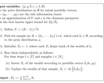
Input variables: (µ, y,˜b, , γ, δ, R)

µis the prior distribution on B for initial portfolio vectors

y= (y1,· · · , yT) are the side information states

˜

b is an approximation ofb∗ and is the closeness parameter

R is the best known upper bound for S_T∗/SˆT

1. Define N := (R−1)/γ2δ.

2. Pick the sample setB={b1,· · · , bN}i.i.d. where eachbi ∈ B, according

to the prior distribution µ.

3. Initialize Xi ←1, where eachXi keeps track of the wealth of bi.

4. Run them independently as follows:

For time steps t∈[T] and samples i∈[N],

(a) InvestXi of the wealth according to portfolio vector ˜b(bi, yt).

(b) Update the wealth of that sample, Xi←St

˜_b₍_b_i₎_.

[image:36.595.129.490.90.378.2]

Output: ˇST := _N1 PNi=1Xi

Figure 3.2: Randomized approximation

by Blum and Kalai [BK99] which approximated Cover’s universal portfolio

(without side information).

It will later become clear as to the particular choice ofN in the Figure 3.2.

The input variables γ and δ in the algorithm above will directly control the

accuracy of the approximation. In particular, the algorithm in Figure 3.2 achieves a wealth of at least 1−γ times as large as the universal portfolio with probability 1−δ. To prove this, we will make use of the one-sided version of Chebyshev’s inequality (otherwise known as Chebyshev-Cantelli) as in the lemma below.

Lemma 5 For a random variable X and for any a >0,

Pr[X≤_E[X]−a]≤ Var[X]

Var[X] +a2.

(37)

Theorem 6 With probability at least1−δ, the approximation from Figure 3.2 achieves a wealthSˇT of at least 1−γ times as large as SˆT. In other words,

Pr ˇ

ST

ˆ

ST

>1−γ

≥1−δ.

This requires sample complexity

O ((1 +c)T)

k(m−1)

γ2_δ

!

.

Proof. As in the algorithm, let Xi represent the wealth derived from the ith

sample bi, where thebi’s are chosen i.i.d. according to µ,

Xi =ST

˜_b₍_b_i₎_.

For someγ, δ ∈[0,1], let

N = (R−1)/γ2δ

whereR is an upper bound for S_T∗/SˆT. Define

X= 1

N

X

i=1 Xi.

Then by linearity of expectation and variance,

E[X] =E[Xi]

and

Var[X] = Var[Xi]/N.

We want to prove that

Pr ˇ

ST

ˆ

ST

>1−γ

≥1−δ,

which is equivalent to

Pr

X

E[X]

≤1−γ

≤δ,

since ˇST = X and ˆST = E[Xi] = E[X]. Re-arranging this and applying

(38)

Lemma 5 we get

Pr [X≤E[X]−γE[X]]≤ Var[X]

Var[X] + (γE[X])2

= Var[Xi] Var[Xi] +N(γE[X])2

,

where the last equality is due to Var[X] = Var[Xi]/N. Therefore it remains

to show that

Var[Xi]

Var[Xi] +N(γE[X])2 ≤δ,

which is equivalent to

Var[Xi](1−δ)

δ(γE[X])2

≤N,

since we assume E[X]>0. We can bound this as

Var[Xi](1−δ)

δ(γE[X])2 =

Var[Xi](1−δ)

δγ2_E[_X

i]2

, sinceE[X] =E[Xi]

≤ Var[Xi]

δγ2_E_[_X

i]2

, sinceδ≥0

= E[X

2

i]−E[Xi]2

δγ2_E_[_X

i]2

, by definition of variance

= 1

γ2_δ

E[Xi2]

E[Xi]2 −1

.

Using the fact that E[Xi] = ˆST and E[Xi2]≤SˇTSˆT, we get

1

γ2_δ

E[Xi2]

E[Xi]2 −1

≤ 1

γ2_δ

ˇ

STSˆT

ˆ

S_T2 −1

!

= 1

γ2_δ

ˇ ST ˆ ST −1 ≤ 1

γ2_δ

S_T∗

ˆ

ST −1

, since ˇST ≤ST∗ (the best CRP)

≤ R−1

γ2_δ , sinceS

∗

T/SˆT ≤R by definition

= N.

To get a bound on the sample complexity, we need a bound onR. Theorem 4 implies that

(39)

Using this we obtain the sample complexity

N = R−1

γ2_δ ∈O

((1 +c)T)k(m−1)

γ2_δ

!

.

When the number of states kand number of assets m are fixed

(indepen-dent ofT), the sample complexity from the theorem above is polynomial inT, although potentially of high order (depending on k, m). On the other hand,

the sample complexity is exponential inm and k.

Kalai and Vempala [KV02] showed a more efficient randomized

approxi-mation scheme for the classical Cover’s universal portfolio (without side

infor-mation or transaction costs). They derived a random walk sampling algorithm that yields sample complexity that is polynomial inm and of low-order

poly-nomial in T (something like O(T3log2T)). Therefore it may be possible to extend their technique to get a more efficient method than the one presented

here. It should be noted though that this is unlikely to be straightforward;

Kalai and Vempala [KV02] mentioned that they do not know of a way to derive an implementation with the presence of transaction costs (c >0), and

further-more it must account for multiple side information states (possiblyk≥2) and prediction inputs as in our new model.

(40)

(41)

Chapter 4

Dynamic Trading Strategy

In this chapter, we introduced a counterpart to the portfolio selection model

from the last chapter that balances the reward from rebalancing the portfolio (based on information received from a price prediction) against the

transac-tion cost incurred, and find an optimal point in between as to maximise cost

adjusted wealth.

The ideas in this chapter will go beyond the restriction imposed by the

CRP, and instead, we devise a model that is competitive with the best greedy portfolio in a stochastic setting: one that makes the optimal decision as if

it knows the next time step’s price. To do this, we suppose that our model

has access to a price prediction ˜xt (of the next time step, t+ 1) that follows

some probability distribution ˜xt∼ Dt(xt), wherextis the later observed price

change (in the sense that xt is revealed by the adversary after the player

draws the prediction and chooses his portfolio). In this model, we quantify the precise relationship between the expected regret and the accuracy of such

predictions. Note that we allow the prediction accuracy to vary over time, as

reflected by the dependence ofDt on the current time stept. We demonstrate

that for certain probability distributions D_t,

E˜xt∼Dt(xt)

max

xT

=o(T)

is attainable, subject to some restrictions on the accuracy of ˜xt’s: namely, that

the integral of the tail probabilities (of mis-estimation) must converge to zero astgrows. Intuitively, this is equivalent to improving our predictions through

(42)

learning from past outcomes, and the requirement is that the model must be learning at a rate fast enough as to satisfy a certain sufficient condition which

we will later prove.

4.1

Greedy Portfolio

At time t ∈ [T], suppose our model has access to a prediction such that it follows some probability distribution with respect to the later observed price change: that is, ˜xt ∼ Dt(xt). Note that the distribution Dt may depend on

the current time step t (hence, the subscript) and xt, possibly hiding

fur-ther dependencies on additional parameters such as volatility. Based on this prediction, we can compute a portfolio distribution as to optimize the wealth.

Definition 5 For each t ∈ [T], given a predicted price-change x˜t of the

ob-served price change xt such that x˜t∼ Dt(xt) for some probability distribution Dt, the portfolio distribution at time tis specified by

ˆ

bt:= arg maxb∈Bbx˜tθ(ˆbt−1, b, xt−1).

The benchmark model, which we call the optimal greedy portfolio, is defined similarly as, for each time t,

b∗_t = arg max_b_∈Bbxtθ(b∗t−1, b, xt−1).

Note that the above models considers the tradeoff between the transaction

cost of shifting to a “better” portfolio against the expected benefit of doing such a rebalancing given the prediction or actual outcome, respectively. In the

case where the optimization yields multiple solutions, we canonically choose

the one with the least transaction costs. This will be made more precise in Section 4.8.

In the rest of the chapter, we investigate how close the wealth of the

above portfolio model is to the optimal greedy portfolio. As a measure of

performance, we consider the expected regret E[R]. Namely,

Ex˜t∼Dt(xt)

max

xT

(43)

This can be interpreted as enumerating through all possible price predictions ˜

xT and choosing the outcome of price sequence xT that maximises regret for

each choice of ˜xT. Each of these choices of ˜xT occurs with some probability

depending on xT and Dt fort ∈[T], and we take the expectation over these

probabilities.

Note that a bound on the expected-regret will also imply a bound (of the

same order, up to some constant) for the regret with high probability, by

Markov’s inequality. In particular, for all k >0,

Pr [R≤kE[R]]≥1− 1

k.

4.2

Impossibility without Predictions

We assume the existence of predictions because otherwise it is impossible to

achieve sublinear expected regret, as demonstrated in the below theorem.

Theorem 7 If there are no predictions, in particular, no restriction on how ˜

xt relates to xt, then sublinear regret is not achievable,

E[R] = Ω(T).

Proof. Consider the two asset case,m= 2. Suppose the probabilistic trader invests according to the portfolio distribution b ∈ B ⊂ _R2 _{with probability} ft(b) at time t ∈ [T]. Then for each b ∈ B ⊂ R2, the adversary chooses a returns vector gt(b) :=xt at timet∈[T] as

gt(b) =

 



(0,1) ifb(1)≥ 1₂,

(1,0) otherwise.

The first condition is equivalent to b(1)≥ b(2) as they must sum up to one. The equivalent best greedy portfolio in hindsight at timet∈[T] is

ht(b) =

 



(0,1) ifg(b) = (0,1),

(1,0) ifg(b) = (1,0).

(44)

This will yield a single-time step expected wealth for the trader at timet∈[T] of

Z

B

ft(b)·gt(b)dft(b) =

Z

b(1)≥1 2

ft(b)·gt(b)dft(b) +

Z

b(1)<1₂

ft(b)·gt(b)dft(b)

= Z

b(1)≥1 2

ft(b)·(0,1)dft(b) +

Z

b(1)<1₂

ft(b)·(1,0)dft(b)

≤

Z

b(1)≥1 2 1 2, 1 2

·(0,1)dft(b) +

Z

b(1)<1₂

1 2, 1 2

·(1,0)dft(b)

= 1 2,

where last inequality is due to the fact that the best portfolio within the constraints that maximises wealth is 1₂,1₂

in both cases. The single-time

step wealth of the best greedy portfolio at time t∈[T] is

Z

B

ht(b)·gt(b)dft(b) =

Z

b(1)≥1 2

ht(b)·gt(b)dft(b) +

Z

b(1)<1₂

ht(b)·gt(b)dft(b)

= Z

b(1)≥1 2

(0,1)·(0,1)dft(b) +

Z

b(1)<1 2

(1,0)·(1,0)dft(b)

= 1.

Therefore, the single-time step expected wealtlh ratio is at least 2. Combining this overT time steps give at least a linear expected regret.

Therefore, the key ingredients to achieving a good performance (against

the optimal greedy portfolio) are accurate price predictions.

4.3

Expected Regret Bound

We analyze the expected regret E[R], where the choice of portfolio distribu-tions depend directly on the random predicdistribu-tions ˜xt∼ Dt(xt) and xt is chosen

adversarially, for eacht∈[T]. The theorem below gives an upper bound on the expected regret of the strategy from Definition 5 against the optimal greedy portfolio as a function of the distributionsDtof predictions in each time step,

(45)

Theorem 8 The expected regret of the portfolio strategy from Definition 5 can be bounded from above as

E[R]≤γ+ 2

T

X

t=1

Z ∞

0

Pr

˜

xt∼Dt(xt)

[˜xt6∈(e−zxt, ezxt)]dz ,1

where γ accounts for the regret arising from the positioning error of the port-folio and is defined as

γ =−

T

X

t=1

E "

logθ(ˆbt−1, b ∗

t, xt−1) θ(b∗_t₋₁, b∗_t, xt−1)

#

.

Proof. We fix some time t and consider the ratio of the single-time-step wealth change of our portfolio to that of the benchmark at time t in order to bound the regret arising from that time step. The regret associated with

the time stepthas two sources: positioning error of the current portfolio that

results in transaction costs and inaccurate price predictions. We define

ρt=

θ(ˆbt−1, b∗t, xt−1) θ(b∗_t₋₁, b∗_t, xt−1)

to capture the regret arising from the positioning error of the portfolio at time

step t: for example, whenb∗_t−1 was in a better position than ˆbt−1 to minimise

transaction costs when rebalancing at timet. Now, suppose that2

(1−δ)xtx˜t(1−δ)−1xt,

at time stept, for someδsuch that 0≤δ <1. Then, for any ˆbt, bt∗,ˆbt−1, b∗t−1 ∈

B, we have the following bound on the ratio of the single-time-step wealths:

ˆ_b_t_x_t_θ_(ˆ_b_t₋₁_,ˆ_b_t_{, x}_t₋₁₎

b∗_txtθ(b∗t−1, b∗t, xt−1)

≥(1−δ)ˆbtx˜tθ(ˆbt−1,ˆbt, xt−1)

(4.1)

≥(1−δ)2ˆbtx˜tθ(ˆbt−1,ˆbt, xt−1)

b∗_tx˜tθ(bt∗−1, b∗t, xt−1)

(4.2)

≥(1−δ)2ρt. (4.3)

1

The notations6∈is applied as a component-wise conjunction, ande−z, ez multiplies on to each element ofxt, sincext,x˜t are multidimensional.

2_{The notations}_,_,_≺_{, and}_{denote component-wise vector inequalities.}

(46)

In the above, (4.1) is due to

xt(1−δ)˜xt,

(4.2) is due to

˜

xt(1−δ)xt,

and (4.3) is due to the fact that

ˆ

btx˜tθ(ˆbt−1,ˆbt, xt−1)≤b∗tx˜tθ(ˆbt−1, b∗t, xt−1)

=ρtb∗tx˜tθ(b∗t−1, b

∗

t, xt−1),

as ˆbt was chosen to maximise its single-time-step wealth by Definition 5. For

each time step t∈[T], we define deviationδtof xt and ˜xt as

δt:= min{δ ≥0|(1−δ)xtx˜t(1−δ)−1xt}.

Intuitively, this is the deviation of the predicted price change from the observed

price change. We can now calculate the expected regret as follows.

E[R] =E

max

xT log

S_T∗

ˆ

ST

=E "

max

xT log

T

Y

t=1

ˆ_b_t_x_t_θ_(ˆ_b_t₋₁_,ˆ_b_t_{, x}_t₋₁₎ !#

≤_E

" log

T

Y

t=1

(1−δt)−2ρ−t1

!#

(4.4)

≤ T

X

t=1

2E[−log(1−δt)]−E[logρt], (4.5)

where (4.4) is by the inequality from (4.3), and (4.5) follows from linearity of

expectation. We now will now use

γ =−

T

X

t=1

(47)

to denote the “positioning error,” and continue our analysis of the first term on the right hand side of the inequality.

T

X

t=1

E[−log(1−δt)] = T X t=1 Z ∞ 0 Pr ˜ xt

[−log(1−δt)≥z]dz

= T X t=1 Z ∞ 0 Pr ˜ xt

[1−δt≤e−z]dz,

= T X t=1 Z ∞ 0

1−Pr

˜

xt

[1−δt> e−z]dz,

= T X t=1 Z ∞ 0

1−Pr

˜

xt

[e−zxt≺x˜t≺ezxt]dz,

where the last line above is obtained from applying the definition ofδt, giving

us the bound on expected regret.

Note that γ from Theorem 8 captures the positioning error of our model

arising from transaction costs. Hence, in the absence of transaction costs (that is, whenc= 0), we have thatγ = 0. In fact, we later prove in Section 4.4 that,

in general, γ = Ω(T) for non-zero transaction costs (that is, when c >0), by

showing that there exists a sequencexT that yields an expected regret at least linear in T.

We also observe thatγ = 0 in the weaker case whenxtis a random variable

that is independent ofxt−1 (hence, also independent of bt∗−1 and ˆbt−1), for all

time steps t∈[T], whereas Theorem 8 is stronger as it makes no assumption on how xt are chosen. This is because

Elogθ(b∗t−1, b∗t, xt−1)

=E

h

logθ(ˆbt−1,ˆbt, xt−1)

i

,

intuitively meaning that the random choice of xt and ˜xt are just as likely be

favourable tob∗_t₋₁ as it is to ˆbt−1. For example, suppose that we define

˜

xt= (1, . . . ,1)

and xt is drawn from some log-normal distribution with mean ˜xt. Then, this

is equivalent to assuming that the returns xt follows a Geometric Brownian

(48)

Motion and that the current price is the best prediction of the next time step’s price; similar to the assumption underlying much of the work in financial

mathematics.

Finally, settingγ aside, the result above gives us a good intuition on what

the expected regret looks like. Namely, in each time step the regret can be thought of to be no larger than the sum of an integral of the tail probabilities.

Having a small expected regret then hinges on efficiently bounding these tail

probabilities.

4.4

Non-zero Transaction Cost

We will now show that for any class of non-trivial distributionsD_t, the expected-regret bound above will not be sublinear for non-zero transaction cost (in ef-fect, showing that γ is necessarily linear inT, for any c >0). This is because

there exists a sequence of returns xt fort∈[T] that will favour b∗t’s position,

hence, yielding a large enough regret.

Here, we define anon-trivial distribution as one where the preimage of the cumulative distribution function is non-empty at some value inside a constant

interval around 1₂. Note that any class of continuous distributions satisfies this

criteria.

Theorem 9 Given non-trivialD_t for all t∈[T], when c >0,

E[R] = Ω(T).

Proof. To prove that the expected regret is not necessarily sublinear in the case of non-zero transaction cost, it is enough to come up with a sequence ofxt

that breaks this sub-linearity. Therefore, we will give a way to construct such

xt for each t∈[T] in the two-asset case (m= 2), where b∗t and ˆbt will always

take the values of either (0,1) or (1,0) by our construction of the re-balancing

scheme from Section 4.8.

First we will describe the proof concept qualitatively, then subsequently

provide the precise details. We will choose xt in such a way that, when our

(49)

loss by making our portfolio rebalance (due to holding the asset with inferior next timestep return). On the other hand, when our portfolio agrees with

that of the competing benchmark, we will choose an xt as to result in equal

probability of rebalancing or staying put, depending on the random variable ˜

xt ∼ Dt(xt). This would imply that, in the long run, our portfolio disagrees

with the competing benchmark in a fixed proportion of the timesteps.

Sum-ming up the fixed loss in these timesteps yield linear regret.

Now we give the formal proof. For time step t, assume that ˆbt−1 = (0,1),

without loss of generality, with b∗_t₋₁ is (0,1) or (1,0). We will calculate the single-time-step loss

ˆ

btxtθ(ˆbt−1,ˆbt, xt−1)

in these two cases separately.

State 1 (Different) b∗_t₋₁ = (1,0)

The adversary choosesxt= (1,1−c), resulting in a single-time-step loss

of ₁₋1_c, regardless of the choice ˜xt∼ Dt(xt).

State 2 (Same) b∗_t₋₁ = (0,1)

The adversary choosesxt= (ξt,1), where ξt is chosen such that

Pr

˜

xt∼Dt((ξt,1))

˜

xt(1)

˜

xt(2)

> 1

1−c

= 1

2.

Intuitively, this is the choice of price relative vector where the portfolio model (as represented by ˆbt) has equal probabilities of shifting or staying

put. This implies that Pr˜xt∼Dt(xt)[ˆbt=b

∗

t] = 12, and the single-time-step

loss may be as small as 1 in this case. Note that this choice ofξtexists if

the preimage of the CDF ofD_tat 1₂ is non-empty. One can easily extend this proof to cases where the preimage of the CDF is non-empty at some

value inside a constant interval around 1₂.

With this information, we can model the dynamics of the portfolio as a Markov chain with these two states (Different and Same)

Algorithmic learning from financial predictions