University of Huddersfield Repository
Somaraki, Vassiliki
A framework for trend mining with application to medical data
Original Citation
Somaraki, Vassiliki (2013) A framework for trend mining with application to medical data.
Doctoral thesis, University of Huddersfield.
This version is available at http://eprints.hud.ac.uk/id/eprint/23482/
The University Repository is a digital collection of the research output of the
University, available on Open Access. Copyright and Moral Rights for the items
on this site are retained by the individual author and/or other copyright owners.
Users may access full items free of charge; copies of full text items generally
can be reproduced, displayed or performed and given to third parties in any
format or medium for personal research or study, educational or notforprofit
purposes without prior permission or charge, provided:
•
The authors, title and full bibliographic details is credited in any copy;
•
A hyperlink and/or URL is included for the original metadata page; and
•
The content is not changed in any way.
For more information, including our policy and submission procedure, please
contact the Repository Team at: [email protected].
A FRAMEWORK FOR TREND MINING WITH
APPLICATION TO MEDICAL DATA
VASSILIKI SOMARAKI
A thesis submitted to the University of Huddersfield in partial fulfilment of the requirements for the degree of Doctor of Philosophy
The University of Huddersfield in collaboration with Eye and Vision Science Department, University of Liverpool & Saint’ Paul Eye Unit, Royal Liverpool University Hospital
2 Copyright statement
The author of this thesis (including any appendices and/or schedules to this thesis) owns any copyright in it (the “Copyright”) and s/he has given The University of Huddersfield the right to use such copyright for any administrative, promotional, educational and/or teaching purposes.
Copies of this thesis, either in full or in extracts, may be made only in accordance with the regulations of the University Library. Details of these regulations may be obtained from the Librarian. This page must form part of any such copies made.
3
Abstract
This thesis presents research work conducted in the field of knowledge discovery. It presents an integrated trend-mining framework and SOMA, which is the application of the trend-mining framework in diabetic retinopathy data. Trend mining is the process of identifying and analysing trends in the context of the variation of support of the
association/classification rules that have been extracted from longitudinal datasets. The integrated framework concerns all major processes from data preparation to the extraction of knowledge. At the pre-process stage, data are cleaned, transformed if necessary, and sorted into time-stamped datasets using logic rules. At the next stage, time-stamp datasets are passed through the main processing, in which the ARM technique of matrix algorithm is applied to identify frequent rules with acceptable confidence. Mathematical conditions are applied to classify the sequences of support values into trends. Afterwards, interestingness criteria are applied to obtain interesting knowledge, and a visualization technique is proposed that maps how objects are moving from the previous to the next time stamp.
A validation and verification (external and internal validation) framework is described that aims to ensure that the results at the intermediate stages of the framework are correct and that the framework as a whole can yield results that demonstrate causality. To evaluate the thesis, SOMA was developed.
4
Table of Contents
Abstract ... 3
Table of Contents ... 4
List of Figures ... 7
List of Tables ... 11
Dedications and Acknowledgements ... 15
Chapter 1 Introduction ... 16
1.1 Contribution and research questions ... 19
1.2 Thesis Structure ... 22
1.3 Publications ... 23
Chapter 2 Literature review ... 25
2.1 Introduction ... 25
2.2 Knowledge discovery in databases process ... 26
2.3 Data Mining methods... 27
2.4 Association Rule Mining ... 30
2.4.1 Apriori algorithm ... 31
2.4.2 Dynamic item-set counting ... 33
2.4.3 Partition ... 34
2.4.4 Frequent pattern growth ... 35
2.4.5 Confidence-based approach ... 36
2.4.6 Matrix algorithm ... 37
2.4.7 Multiple supports Apriori ... 38
2.4.8 Hash-based technique and pruning ... 39
2.4.9 Eclat algorithm ... 40
2.4.10 Sampling technique ... 40
2.4.11 Measuring interestingness of rules ... 41
2.5 Associative classification ... 42
5
2.7 Temporal Logic ... 45
2.8 Longitudinal data mining ... 46
2.9 Data mining for medical applications ... 46
2.10 Trend mining ... 50
2.11 Validation and verification ... 53
2.12 Conclusion ... 55
Chapter 3 Medical Overview and Data Description ... 56
3.1 Introduction ... 56
3.2 Diabetes overview ... 58
3.3 Diabetic Retinopathy overview ... 59
3.4 Epidemiology ... 62
3.5 Symptoms ... 63
3.6 Data collection and pre-processing ... 64
3.6.1 Diabetic retinopathy Databases ... 65
3.6.2 Data warehousing and cleaning... 68
3.6.3 Issues and challenges of medical data ... 70
3.7 Conclusion ... 74
Chapter 4 Trend-mining framework description ... 75
4.1 Introduction ... 75
4.2 Trend mining framework ... 76
4.2.1 Pre-processing ... 77
4.2.2 Main processing ... 77
4.2.3 Representation of the trends ... 83
4.3 SOMA: An application of trend mining in diabetic retinopathy ... 83
4.4 Validation and verification of the Framework ... 90
4.4.1 Verification ... 91
4.4.2 Validation ... 93
4.5 Conclusion ... 97
Chapter 5 Evaluation... 98
6
5.2 Verification experiments ... 99
5.3 Validation of the trend mining framework... 114
5.3.1 Validation experiments ... 114
5.4 Evaluation of the trend mining framework ... 120
5.4.1 Criteria discussion ... 121
5.4.2 Criteria implementation ... 122
5.4.3 Experimental set-up ... 125
5.4.4 Experimental results and evaluation ... 126
5.4.4.1 Noise reduction ... 127
5.4.4.2 Object distribution ... 129
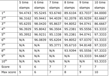
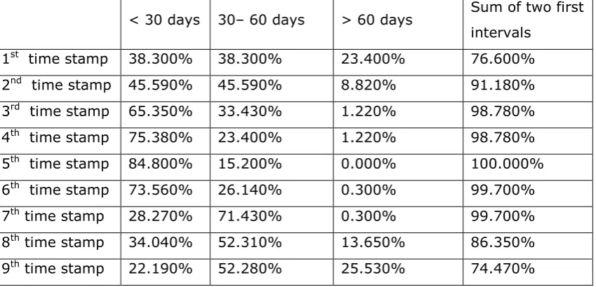
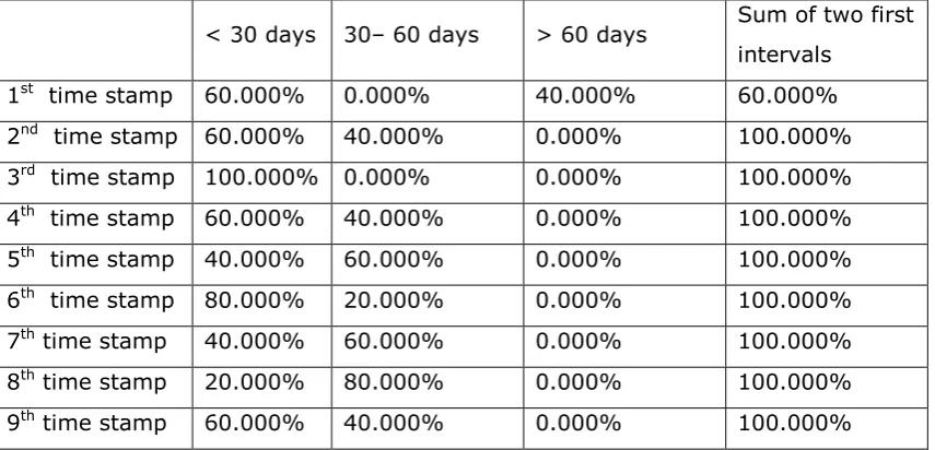
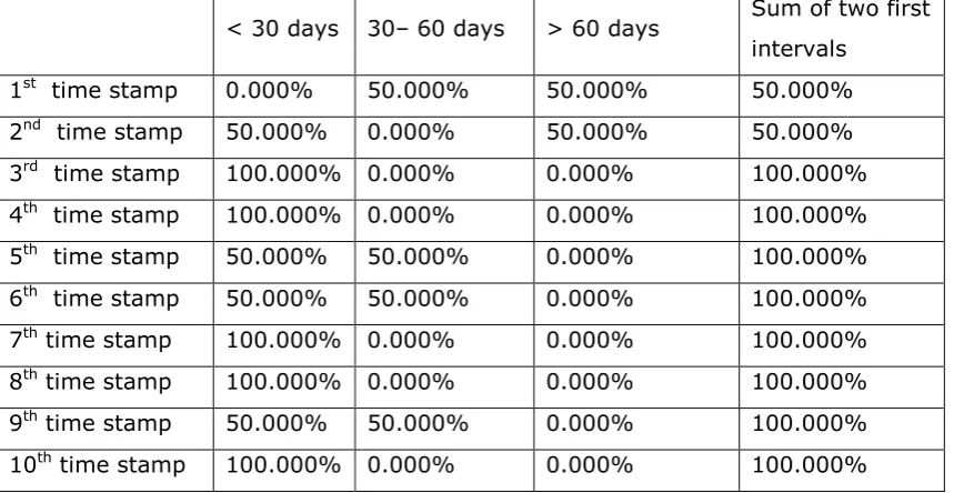
5.4.4.3 Time-stamp distribution ... 131
5.4.4.4 Interestingness ... 149
5.4.4.5 Quality of the knowledge discovered ... 156
5.4.5 Discussion ... 158
Chapter 6 Conclusion & Future Work ... 162
6.1 Future work ... 163
Appendices ... 165
Appendix 1 – Schemas for logic rules ... 165
Appendix 2 – Noise reduction ... 238
Appendix 3 – Time stamp interval distribution ... 246
Appendix 4 – Trends representation ... 264
7
List of Figures
Figure 2.1 :Overview of the KDD process (Fayyad, Piatetsky-Shapiro, and Smyth 1996a) 26
Figure 2.2 :Techniques for DM (Han et al., 2011) ... 28
Figure 2.3 :Apriori Algorithm...32
Figure 2.4 : Apriori Generate_Candidate function...32
Figure 2.5 : Apriori candidate generation example...33
Figure 3.1 :Circulatory system of the retina ... 60
Figure 3.2 :Mechanism of DR development ... 61
Figure 3.3 :Photograph of a normal eye, with no DR ... 62
Figure 3.4 : Photograph of an eye with DR... 62
Figure 4.1: Trend mining framework presentation...76
Figure 4.2: Patient distribution based on the time interval from the previous to the next episode...85
Figure 4.3 : Timeline of episodes creation...85
Figure 4.4: How framework reads data...88
Figure 5.1: Pair of Disappearing and Jumping trends...117
Figure 5.2: Pair of decreasing and increasing trends...119
Figure A2.1: Noise reduction – 5 time stamps – Series 1...238
Figure A2.2: Noise reduction – 6 time stamps – Series 1...238
Figure A2.3: Noise reduction – 7 time stamps – Series 1...239
Figure A2.4: Noise reduction – 8 time stamps – Series 1...239
Figure A2.5: Noise reduction – 9 time stamps – Series 1...240
Figure A2.6: Noise reduction – 10 time stamps – Series 1...240
Figure A2.7: Noise reduction – 5 time stamps – Series 2...241
Figure A2.8: Noise reduction – 6 time stamps – Series 2...241
Figure A2.9: Noise reduction – 7 time stamps – Series 2...242
Figure A2.10: Noise reduction – 8 time stamps – Series 2...242
Figure A2.11: Noise reduction – 9 time stamps – Series 2...243
Figure A2.12: Noise reduction – 10 time stamps – Series 2...243
Figure A2.13: Noise reduction – 5 time stamps – Series 3...244
Figure A2.14: Noise reduction – 6 time stamps – Series 3...244
Figure A2.15: Noise reduction – 7 time stamps – Series 3...245
Figure A2.16: Noise reduction – 8 time stamps – Series 3...245
Figure A3.1: Patient distribution in intervals for every time stamp, from General to Photodetails – Series 1...246
8 Figure A3.3: Patient distribution in intervals for every time stamp, from General to
Photodetails – Series 3...247 Figure A3.4 :Patient distribution in intervals for every time stamp, from General to
Photodetails – Series 1...247 Figure A3.5 :Patient distribution in intervals for every time stamp, from General to
Photodetails – Series 2...248 Figure A3.6: Patient distribution in intervals for every time stamp, from General to
Photodetails – Series 3... 248 Figure A3.7: Patient distribution in intervals for every time stamp, from General to
Photodetails – Series 1... 249 Figure A3.8: Patient distribution in intervals for every time stamp, from General to
Photodetails – Series 2... 249 Figure A3.9: Patient distribution in intervals for every time stamp, from General to
Photodetails – Series 3... 250 Figure A3. 10 :Patient distribution in intervals for every time stamp, from General to
Photodetails – Series 1 ... 250 Figure A3. 11 :Patient distribution in intervals for every time stamp, from General to
Photodetails – Series 2 ... 251 Figure A3. 12 distribution in intervals for every time stamp, from General to Photodetails – Series 3 ... 251 Figure A3. 13 :Patient distribution in intervals for every time stamp, from General to
Photodetails – Series 1 ... 252 Figure A3.14: Patient distribution in intervals for every time stamp, from General to
Photodetails – Series 2...252 Figure A3. 15 :Patient distribution in intervals for every time stamp, from General to
Photodetails – Series 3 ... 253 Figure A3.16: Patient distribution in intervals for every time stamp, from General to
Photodetails – Series 1...253 Figure A3.17: Patient distribution in intervals for every time stamp, from General to
Photodetails – Series 2...254 Figure A3.18: Patient distribution in intervals for every time stamp, from General to
11
List of Tables
Table 4.1: Mathematical conditions for trend categorization...82
Table 4.2: SOMA output language...94
Table 5.1: Number of patients per number of episodes...99
Table 5.2: Experimental conditions...101
Table 5.3: Experimental conditions...101
Table 5.4: Experimental conditions...101
Table 5.5: Experiment A...102
Table 5.6 : Experiment B...102
Table 5.7 : Experiment C...103
Table 5.8 : Experiment D...103
Table 2.9 : Experiment E...104
Table 5.10 : Experiment F...104
Table 5.11 : Experiment G...105
Table 5.12 : Experiment H...105
Table 5.13 : Experiment I...106
Table 5.14 : Experiment K...106
Table 5.15 : Experiment L...107
Table 5.16 : Experiment M...107
Table 5.17 : Experiment N...108
Table 5.18 : Experiment O...108
Table 5.19 :Experiment P...109
Table 5.20 : Experiment Q...109
Table 5.21 : Experiment R...110
Table 5.22 : Experiment S...110
Table 5.23 :Experiment T...111
Table 5.24 : Experiment U...111
Table 5.25 :Experiment V...112
Table 5.26 : Experiment W...112
Table 5.27: Experiment X...113
Table 5.28 : Experiment Y...113
Table 5.29: Experimental Parameters...126
Table 5.30: Dataset size...127
Table 5.31: Noise reduction (%) for series 1...128
Table 5.32: Noise reduction (%) for series 2...128
Table 5.33: Noise reduction (%) for series 3...129
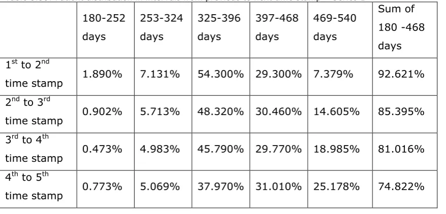
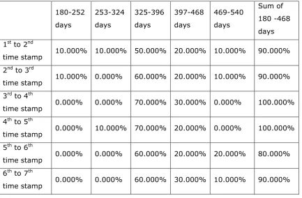
12 Table 5.35: Patient distribution (%) for series 2...130 Table 5.36: Patient distribution (%) for series 3...131 Table 5.37: Patient distribution in intervals for every time stamp, from General to
Photodetails – Series 1...132 Table 5.38: Patient distribution in intervals for every time stamp, from General to
Photodetails – Series 2...132 Table 5.39: Patient distribution in intervals for every time stamp, from General to
Photodetails – Series 3...132 Table 5.40: Patient distribution in intervals for every time stamp, from General to
Photodetails – Series 1...132 Table 5.41: Patient distribution in intervals for every time stamp, from General to
Photodetails – Series 2...133 Table 5.42: Patient distribution in intervals for every time stamp, from General to
Photodetails – Series 3...133 Table 5.43: Patient distribution in intervals for every time stamp, from General to
Photodetails – Series 1...133 Table 5.44: Patient distribution in intervals for every time stamp, from General to
Photodetails – Series 2...134 Table 5.45: Patient distribution in intervals for every time stamp, from General to
Photodetails – Series 3...134 Table 5.46: Patient distribution in intervals for every time stamp, from General to
Photodetails – Series 1...134 Table 5.47: Patient distribution in intervals for every time stamp, from General to
Photodetails – Series 2...135 Table 5.48: Patient distribution in intervals for every time stamp, from General to
Photodetails – Series 3...135 Table 5.49: Patient distribution in intervals for every time stamp, from General to
Photodetails – Series 1...135 Table 5.50: Patient distribution in intervals for every time stamp, from General to
Photodetails – Series 2...136 Table 5.51: Patient distribution in intervals for every time stamp, from General to
Photodetails – Series 3...136 Table 5.52: Patient distribution in intervals for every time stamp, from General to
Photodetails – Series 1...136 Table 5.53: Patient distribution in intervals for every time stamp, from General to
Photodetails – Series 2...137 Table 5.54: Patient distribution in intervals for every time stamp, from General to
13 Table 5.55: Score summary for series 1; from General to Photodetails...138 Table 5.56: Score summary for series 2; from General to Photodetails...138 Table 5.57: Score summary for series 3; from General to Photodetails...138 Table 5.58: Patient distribution in intervals from previous to next time stamp –
Series 1...139 Table 5.59: Patient distribution in intervals from previous to next time stamp –
Series 2...140 Table 5.60: Patient distribution in intervals from previous to next time stamp –
Series 3...140 Table 5.61: Patient distribution in intervals from previous to next time stamp –
Series 1...140 Table 5.62: Patient distribution in intervals from previous to next time stamp –
Series 2...141 Table 5.63: Patient distribution in intervals from previous to next time stamp –
Series 3...141 Table 5.64: Patient distribution in intervals from previous to next time stamp –
Series 1...142 Table 5.65: Patient distribution in intervals from previous to next time stamp –
Series 2...142 Table 5.66: Patient distribution in intervals from previous to next time stamp –
Series 3...143 Table 5.67: Patient distribution in intervals from previous to next time stamp –
Series 1...143 Table 5.68: Patient distribution in intervals from previous to next time stamp –
Series 2...144 Table 5.69: Patient distribution in intervals from previous to next time stamp –
Series 3...144 Table 5.70: Patient distribution in intervals from previous to next time stamp –
Series 1...145 Table 5.71: Patient distribution in intervals from previous to next time stamp –
Series 2...145 Table 5.72: Patient distribution in intervals from previous to next time stamp –
Series 3...146 Table 5.73: Patient distribution in intervals from previous to next time stamp –
Series 1...146 Table 5.74: Patient distribution in intervals from previous to next time stamp –
14
Series 3...147
Table 5.76: Score summary for series 1; from General to Photodetails...148
Table 5.77: Score summary for series 2; from General to Photodetails...148
Table 5.78: Score summary for series 3; from General to Photodetails...148
Table 5.79: Summary of interestingness score for series 1...151
Table 5.80: Summary of interestingness score for series 2...151
Table 5.81: Summary of interestingness score for series 3...152
Table 5.82: Interestingness score for series 1...153
Table 5.83: Interestingness score for series 2...154
Table 5.84: Interestingness score for series 3...155
Table A1.1 :Schema for DiabRetinaPhotodetails dataset...165
Table A1.2: Schema for General Dataset...193
15
Dedications and Acknowledgements
I would like to express my deep and profound gratitude to my principal supervisor, Professor Lee Mc Cluskey, who has always supported my ideas and encouraged their pursuit, and also for his invaluable advice, guidance, and extensive revision of the thesis. He was endlessly patient with me, and I am deeply grateful to him.
I also would like to express my appreciation to my second supervisor, Professor Simon P. Harding, Head of the Department of Eye and Vision Science, for his support,
suggestions, and valuable comments, and for his support with the honorary contract with the NHS St Paul’s Eye Unit of the Royal Liverpool University Hospital. Special thanks also to all the staff in the Department of Computer and Engineering at The University of Huddersfield and the St. Paul’s Eye Unit at the Royal Liverpool University Hospital, who have been helpful whenever needed. I am also very thankful to Professor Deborah Broadbent, Director of Diabetes in Department of Eye and Vision Science, Royal
Liverpool Hospital, who has been helpful in providing advice many times during my work on databases. Special thanks to other members of staff of the University of the
Huddersfield especially to Professor Joan Lu and Dr Di Cai for their valuable help and advice during my studies. I would like also to thank deeply Dimitrios Tsaltas and Thomas Politis with their support and valuable advices during my studies.
16
Chapter 1 Introduction
Ignorance is the curse of God, knowledge the wing wherewith we fly to heaven— William Shakespeare
We now live in the information age. “Data owners” such as scientists, businesses, and medical researchers, are able to gather, store, and manage previously unimaginable
quantities of data owing to technological advances and economic sciences in sensors, digital memory, and data-management techniques. In 1991, it was proposed that the amount of data stored in the world doubles every 20 months (Piatetsky-Shapiro and Frawley, 1991). At the same time, there is a growing realization and expectation that data, intelligently analysed and presented, will be a valuable resource to gain a competitive advantage.
Knowledge Discovery (KD) is a non-trivial process of identifying valid, novel, potentially useful, and ultimately understandable patterns from large collections of data (Fayyad et al., 1996). One of the steps KD is Data Mining (DM). DM is concerned with the actual extraction of knowledge from data, in contrast to the KD process, which is concerned with many other things such as understanding and preparation of the data, verification, and application of the discovered knowledge. In practice, however, people use terms DM, KD, and DMKD synonymously (Cios et al., 2002). The design of a framework for a KD process is an
important issue. Several researchers have described a series of steps that constitute the KD process, ranging from very simple models, incorporating few steps that usually include data collection and understanding, DM, and implementation, to more sophisticated models such as the nine-step model proposed by Fayyad et al. (1996) or the six-step DMKD process model proposed by Cios et al. (2000) and Cios and Moore (2000). Cios et al. (2000) applied the model to several medical problem domains (Sacha et al., 2000; Kurgan et al., 2001, 2003).
To bridge the growing gap between data generation and data understanding, there is an urgent need for new computational theories and tools to assist humans in extracting useful knowledge from the huge volumes of data. These theories and tools are the subject of the emerging field of Knowledge Discovery in Databases (KDD), or DM, which sits at the common frontiers of several attributes including Database Management, Artificial
Intelligence, Machine Learning, Pattern Recognition, and Data Visualization (Hand, 1994).
17 knowledge-based systems, artificial intelligence, high performance computing, and data visualization” (Han and Kamber, 2006).
In the past decade, DM techniques have been widely applied in bioinformatics (Wang et al., 2005), e-commerce (Raghavan, 2005), financial studies (Kovalerchun and Vityaev, 2000), geography (Miller and Han, 2001), marketing and sales studies (Berry and Linoff, 1997; Rypielski et al., 2002), etc.
Most DM applications routinely require datasets that are considerably larger than those that have been addressed by traditional statistical procedures. The size of the datasets often means that traditional statistical algorithms are too slow for DM problems, and alternatives have to be devised. The volume of the data is probably not very important: the number of variables or attributes often is much more important. The analysis of the way in which data change with time is an important mechanism for providing information for decision-makers, policy-makers and other “stakeholders”. One way of conducting such an analysis is by considering data trends.
Trends can be defined and generated in a number of ways. One mechanism, and the focus of the work to be undertaken here, is to define trends in terms of the way that the
frequency of occurrence of patterns changes with time and to employ DM techniques to identify such trends. In this work, the term “trend mining” has been adopted to describe this discovery process.
Trend mining is the process of identifying and analysing trends in the context of the
variation of the support of the association rules that have been extracted from longitudinal datasets. The proposed trend-mining mechanism is founded on an Association Rule Mining (ARM) approach whereby an ARM technique is applied to a sequence of time-stamped data sets. This approach is both efficient and effective in finding trends.
The temporal data to which trend mining can be applied can take many forms; one common form of data is longitudinal data. One application domain that features data sets that are both large and temporal is medical records or, more specifically, patient records. Many branches of medicine have collected large longitudinal data sets spanning many years. These data sets in themselves constitute a wealth of information.
18 The field of medical informatics has evolved around structuring, processing, storing, and transmitting medical information for a variety of purposes (Shortliffe, 1990). One of these purposes is to develop decision-support systems that enhance the human ability to
diagnose, treat, and assess prognoses of pathological conditions. Even if disease processes were fully understood, population variability would still make individualized diagnosis, treatment, and prognosis— all essential parts of good health care—difficult classification tasks. The reality is, however, that diseases are not fully understood; nor is population variability fully taken into account in many decision-making situations. Sometimes it is not possible for a clinician to employ the principles learned in the basic and clinical sciences to determine whether a patient has a given disease, whether he or she should be given a certain treatment, and how long he or she will survive.
Trends across time-stamped data sets can therefore be identified by observing the change in the support values of items sets across the data set. Trend mining is a branch of DM that focuses on the process of identifying and analysing hidden trends in temporal data. The study described in this work is directed towards longitudinal patient data (longitudinal data are data collected using the same set of attributes at a series of points over time), more specifically diabetic retinopathy screening data collected by St. Paul’s Eye Unit, Royal Liverpool University. Diabetic retinopathy (DR) is a common complication of diabetes, the most common cause of blindness in working-age people in the UK. DR is a chronic disease affecting patients with diabetes mellitus and causes damage to the retina (Kanski, 2007). Over 3,000,000 people suffer from diabetes, at least 750,000 people are registered blind or partially sighted in the UK, and the remainder are at risk of blindness. Consequently, it is important that DR be diagnosed at an early stage, and accurately.
The research objective of the work is to investigate and identify a mechanism or
mechanisms, whereby longitudinal data trends can be mined and the results presented in such a way that informed decisions can be made by policy-makers, etc. Broadly, this entails a number of issues:
The mechanism for the pre-processing of the longitudinal data required to permit the desired trend mining.
The nature of the trend mining mechanisms to be employed.
The identification of the process to be used to present the results in a meaningful way. Longitudinal data thus provide a record of the “progress” of some set of features associated with the subjects. Medical longitudinal data, such as DR data, typically plot the progress of a medical condition.
19 This work has resulted in a novel trend mining framework along with a validation and
verification framework, and also resulted with an evaluation application called “SOMA”, which not only enables trend mining but also supports the validation of discovered trends. This validation is based upon the selection of certain attributes for which there are known associations. Having known these associations as well as the patterns they change, trends can be identified using mathematical conditions. Hence, the main purpose of this research is to develop a novel trend-mining framework for extracting trends from longitudinal data while emphasizing the validation of those trends.
This thesis introduces the described method as a general framework for trend-mining validation and verification that can be applied generally to most trend procedures and types of data. The work also introduces trend mining, provides a description of the validation framework, and includes the experimental evaluation of the application.
1.1 Contribution and research questions
Trend mining remains an open challenge in the field of knowledge discovery in data (KDD). This can be attributed partly to the lack of a clear definition of what we mean by a “trend” (it is very much an application-dependent definition), and partly to issues associated with the modelling of time-stamped (longitudinal) data. This research addresses the
development of a trend-mining framework for knowledge discovery from large databases, the development of a validation framework for trend mining, and the application of trend mining in medical data (SOMA). The trend-mining framework is an integrated platform which can be used for knowledge discovery in databases starting from the pre-processing of data and ending with the extraction of useful information.
The research questions which arise from this research work are:
• What is the most appropriate mechanism to identify, analyse and validate trends in real, noisy and longitudinal data and in particular when the input time stamped data denote patients' progress?
• Can this mechanism produce trends that may be employed for prediction purposes? • Can trend mining be applied on medical applications?
More detailed, this thesis examines the following issues:
• How can frequent patterns and trends be discovered to facilitate the desired trend mining?
• How can changes be detected in the identified trends?
20 • Can be applied constraints to the data in order to anticipate interesting, desirable
and useful trends?
• How can different types of trends be interpreted to the users? • What criteria can be used to validate and verify the framework?
In the pre-processing stage the framework directed to solve issues that they arise after bringing together data from various sources such as missing values, heterogeneity of data (combination of numerical with discrete or continuous values and or categorical data) and creation of time stamps. The creation of time stamped data is very important issue for the framework. The data do not feature a clear association between specific time stamps and subsets of data. These include any time-stamped subset of data comprising data collected at different dates and stored in different locations. As a result, the creation of time-stamped subsets for analysis is not straightforward and they form quasi-longitudinal data.
At the processing stage, the framework, through the combination of association rule mining (ARM) and prototype mathematical conditions, deals with the following challenges:
identifying temporal patterns (associations) that commonly occur in the input data;
working on distinguish interesting knowledge through a large amount of temporal patterns
identifying change points of state changes in temporal sequences or, alternatively, the lack of such state changes;
the grouping (clustering) of data according to some temporal change;
the classification of temporal data sequences.
The knowledge that is extracted from trend mining depicts how the initial conditions (that describe a situation) of a group (e.g. patients) change over time. This type of change is called a state change. To visualize any possible state stage, a colourful representation scheme is used to interpret the results.
This thesis also aims to produce a consistent framework for validation of trend mining. The trend-mining method essentially performs “learning by discovery”, and so it cannot be trained; rather, the user has to have confidence in the results it gives, that is, it should be validated. To perform validation and verification of the trend-mining framework, two complementary approaches are advocated here:
Validation: This method tests the outputs of the framework and also checks the consistency in the application that experts already know and expect. The methods include: confirmation of the framework that uncovers known causal connections in the application and
confirmation of the framework that uncovers known trends in the application.
21 of declarative validation rules are set up, and a systematic process of validation of each set of input data is created.
For the development and application of both the trend-mining framework and its validation framework, real world medical data are used in this research. Data came from the Diabetic Retinopathy databases maintained by the Royal Liverpool University Hospital, and these data are an example of an irregular database in that they contain 150,000 records
comprising 450 attributes distributed over two databases, each composed of a number of tables.
SOMA, the application of the framework over those data, consists of three steps:
Pre-processing: data from different sources are brought together after applying logic rules to deal with problems arising from the nature of data and to create a time-stamped subset for analysis.
ARM stage where, for each time-stamped subset, the matrix algorithm technique is used to identify the rules, which are determined by the user specifying which are “variable attributes”, or the left-hand side of the rule, and which are the key
attributes, or the right-hand side of the rule, whose support and confidence exceeds the user’s specified threshold values. Matrix algorithm (Yuan and Huang, 2005) it is a novel algorithm for the identification of frequent item sets based on the creation of a matrix with binary entries and its main advantage is that only one passing it is needed.
The trend mining taking information from the ARM stage creates trends using prototypes (mathematical conditions), which show the attitude of the rules over time. Beyond this, trend mining creates a colourful representation that shows how a group of patients moving from one time-stamp to another either remain with the same rule or may move to another rule owing to changes in some of their
characteristics.
A novel algorithm was created to implement the above trend mining framework. The algorithm consists of 3 parts: the first part implements pre-processing, the 2nd part is the main processing and the last part is the post-processing and outputting the results.
22
1.2 Thesis Structure
The rest of this thesis is organised as follows:
Chapter 2 presents the literature review which describes the background of current KDD research with respect to a variety of methodologies in both data mining in general and trend mining in particular. Also Review of Association Rule Mining, review of trend mining (similar approaches for identifying change, such as Emerging Patterns and Jumping EPs, to which the work can be compared), review of the nature of longitudinal data.
Chapter 3 presents the Medical overview of Diabetic retinopathy and review of the data used and the challenging aspects of these data, the warehouse, logic rules, and the pre-processing. Draw out the fact that the data being used is different to more standard temporal data sets in terms of the concept of episodes. Include description of methods including definitions and schemas.
Chapter 4 introduces the Trend mining framework and description. An approach to trend mining is to use the concept of user defined temporal prototypes to define the nature of the trends of interests. The trends are defined in terms of sequences of support values associated with identified frequent patterns. The prototypes are defined mathematically so that they can be mapped onto the temporal patterns. A process to validate the intermediate data sets and the results of the trend mining process is presented. This is about how to deal with the main challenge of the framework which is how to evaluate the results of trend mining. The primary information that is required for the validation stage is a set of "expected" associations between features, given that all these features have been represented as inputs. These associations represent actual known relationships between features. The purpose is to produce a consistent framework for validation:
23 sequence of processes are working correctly. The trend mining framework application
SOMA, and Aretaeus, the associated trend mining algorithm have been developed. The application is used to detect different kinds of trends across longitudinal medical datasets. Chapter 5 details the evaluation of research work on trend mining. The aim is to evaluate the approach for the development of the advocated trend mining framework. The goal of evaluation process described here is to judge the usefulness of the discovered knowledge and the process of trend mining itself. On the one hand the evaluation of the produced rules is straightforward by using criteria evaluating novelty action ability
unexpectedness reliability etc, on the other hand evaluating the processes of the framework is based on quantitative criteria which measure the performance. The evaluation by
applying the framework to the DR data examines if the validation and verification are effective as part of the framework.
Chapter 6 conclude the thesis and present a summary of research work along with main findings and future work.
Finally, the Appendices present information on the data used (schemas), tables and figures from evaluation experiments.
1.3 Publications
The following papers were produced as part of the research described in this thesis: Somaraki V., Broadbent D., Harding P.S., Coenen F. (2010). Finding temporal patterns in noisy longitudinal data: A study in diabetic retinopathy. Perner, Petra (ed.), Advances in Data Mining. Applications and Theoretical Aspects. 10th
Industrial Conference, ICDM 2010, Berlin, Germany, July 12-14, 2010.
Proceedings. Berlin: Springer. Lecture Notes in Computer Science 6171. Lecture Notes in Artificial Intelligence, 418–431.
24 Somaraki V., Harding P.S., Broadbent D., Coenen F. (2010).SOMA: A Proposed Framework for Trend Mining in Large UK Diabetic Retinopathy Temporal
Databases. Research and Development in Intelligent Systems XXVII Proceedings of AI-2010, The Thirtieth SGAI International Conference on Innovative Techniques and Applications of Artificial Intelligence Bramer, Max; Petridis, Miltos; Hopgood, Adrian (Eds.)
This paper is a continuation and extension of the previous paper and how the proposed framework is able to detect different kinds of trends within the SOMA application and how the proposed framework is able to detect different kinds of trends within longitudinal datasets. To evaluate the proposed framework the process was applied to a large collection of medical records, forming part of the diabetic retinopathy screening programme at the Royal Liverpool University Hospital.
25
Chapter 2 Literature review
2.1 Introduction
This thesis describes an approach to finding temporal patterns in noisy longitudinal patient data and an extended internal and external validation (validation and
verification) process to validate the framework. The identification of patterns in such data has many applications. One common example is the analysis of questionnaire returns collated over a number of years, for example Kimm et al.,(2000) studied the nature of physical activity in groups of adolescents and Skinner et al. studied children's food eating habits (Skinner et.al,2002).Another example of the application of
longitudinal studies is in the analysis of statistical trends; an early reported example is that of Wagner (1992),who performed an extensive longitudinal study of children with special educational needs". Longitudinal studies particularly lend themselves to the analysis of patient data in medical environments where records of a series of
“consultations" are available. For example Yamaguchi et. al., (2001) studied the effect of treatments for shoulder injuries, and (Levy et, al., 1996) studied the long term effects of Alzheimer's disease.
In this chapter a literature review is presented on topics that are related to the
development of the trend mining framework. Firstly, is given an overview of data mining and also the following aspects are covered:
Association Rule Mining (ARM): they are presented as algorithms for the discovery of association rules in datasets and a set of criteria for the definition of what is an interesting rule.
Associative Classification (AC): how ARM can be used to build a classifier.
Data mining in medical applications or Medical Data Mining(MDM): here it is presented how data mining techniques are applied to extract knowledge from medical data
Trend Mining(TM): here is presented the definition of trend mining and the work on emerging and jumping patterns which are the cornerstone on which a new trend mining algorithm is built.
26
2.2 Knowledge discovery in databases process
Knowledge discovery in databases (KDD) has been attracting a huge amount of research, for business, media, social network, health care, etc. As data volumes have grown dramatically, manual analysis and interpretation of data have become impractical for many domains. KDD is the overall process of discovery of novel, potentially useful, and ultimately understandable patterns in data (Fayyad, Piatetsky-Shapiro, and Smyth 1996a).
The KDD process consists of several steps (Fayyad, Piatetsky-Shapiro, and Smyth 1996b), which are shown in Figure 2.1.
Figure 2.1 :Overview of the KDD process (Fayyad, Piatetsky-Shapiro, and Smyth 1996a)
1. Developing an understanding of the application domain and the relevant prior knowledge and identifying the goal of the KDD process from the user’s viewpoint.
2. Creating a target data set: selecting a data set, or focusing on a subset of variables or data samples, on which discovery is to be performed.
3. Cleaning and pre-processing. Basic operations include removing noise if appropriate, collecting the necessary information to model or account for noise, deciding on strategies for handling missing data attributes, and accounting for time-sequence information and known changes.
27 5. Matching the goals of the KDD process (step 1) to a particular data-mining method. For example, summarization, classification, regression, clustering, and so on.
6. Exploratory analysis and model and hypothesis selection: choosing the data mining algorithm(s) and selecting method(s) to be used for searching for data patterns. This process includes deciding which models and
parameters might be appropriate and matching a particular data-mining method with the overall criteria of the KDD process (for example, the end user might be more interested in understanding the model than its
predictive capabilities).
7. Data mining: searching for patterns of interest in a particular representational form or a set of such representations, including classification rules or trees, regression, and clustering. The user can significantly aid the data-mining method by correctly performing the preceding steps.
8. Interpreting mined patterns: possibly returning to any of steps 1 through 7 for further iteration. This step can also involve visualization of the extracted patterns and models or visualization of the data given the extracted models.
9.
Acting on the discovered knowledge: using the knowledge directly, incorporating the knowledge into another system for further action, or simply documenting it and reporting it to interested parties. This process also includes checking for and resolving potential conflicts with previously believed (or extracted) knowledge.2.3 Data Mining methods
As noted above, data mining (DM) is part of the KDD process, and it is the stage where knowledge discovery takes place. As a highly application driven-domain, DM has
28 Figure 2.2 : Techniques for DM (Han et al., 2011)
Two high-level primary goals of DM in practice tend to be prediction and description. Prediction involves using some variables or attributes in the database to predict unknown or future values of other variables of interest, and description focuses on finding human-interpretable patterns describing the data. Although the boundaries between prediction and description are not always distinct (some of the predictive models can be descriptive to the extent that they are understandable, and vice versa), the distinction is useful for understanding the overall discovery goal. The relative importance of prediction and description for particular DM applications can vary
considerably. The goals of prediction and description can be achieved using a variety of particular DM methods. Some of the methods for DM are described below (Witten and Frank, 2005; Han et al., 2011):
Regression is learning a function that maps a data item to a real-valued prediction variable. There are many regression applications, such as predicting the amount of biomass present in a forest given remotely
sensed microwave measurements, estimating the probability that a patient will survive given the results of a set of diagnostic tests, predicting
consumer demand for a new product as a function of advertising
expenditure, and predicting time series where the input variables can be time-lagged versions of the prediction variable.
29 The classifiers used are generated using what are called supervised
learning methods in that they require pre-labelled training data.
Clustering is a common descriptive task where one seeks to identify a finite set of categories or clusters to describe the data (Jain and Dubes, 1988; Titterington, Smith, and Makov, 1985). The categories can be mutually exclusive and exhaustive, or consist of a richer representation, such as hierarchical or overlapping categories. Examples of clustering applications in a knowledge discovery context include discovering
homogeneous subpopulations for consumers in marketing databases and identifying subcategories of spectra from infrared sky measurements. Closely related to clustering is the task of probability-density estimation, which consists of techniques for estimating from data the joint multivariate probability density function of all the variables or attributes in the
database (Silverman, 1986).
Summarization involves methods for finding a compact description for a subset of data. A simple example would be tabulating the mean and standard deviations for all attributes. More sophisticated methods involve the derivation of summary rules (Agrawal et al., 1996), multivariate visualization techniques, and the discovery of functional relationships between variables (Zembowicz and Zytkow, 1996). Summarization techniques are often applied to interactive exploratory data analysis and automated report generation.
Dependency modelling consists of finding a model that describes
significant dependencies between variables. Dependency models exist at two levels: (1) the structural level of the model specifies (often in graphic form) which variables are locally dependent on each other, and (2) the quantitative level of the model specifies the strengths of the dependencies using a numeric scale. For example, probabilistic dependency networks use conditional independence to specify the structural aspect of the model and probabilities or correlations to specify the strengths of the
dependencies (Glymour et al., 1987; Heckerman, 1996). Probabilistic dependency networks are increasingly finding applications in areas as diverse as the development of probabilistic medical expert systems from databases, information retrieval, and modelling of the human genome.
Decision trees and rules that use univariate splits have a simple
30 approximation power) of the model. A large number of decision tree and rule-induction algorithms are described in the machine learning and applied statistics literature (Quinlan, 1992; Breiman et al., 1984). To a large extent, they depend on likelihood-based model-evaluation methods, with varying degrees of sophistication in terms of penalizing model
complexity. Greedy search methods, which involve growing and pruning rule and tree structures, are typically used to explore the
super-exponential space of possible models. Trees and rules are primarily used for predictive modelling, both for classification (Apte and Hong, 1996; Fayyad, Djorgovski, and Weir, 1996) and for regression, although they can also be applied to summary descriptive modelling (Agrawal et al., 1996).
2.4 Association Rule Mining
Association Rule Mining (ARM) consists of first finding frequent item sets (set of items A and B) from which strong association rules in the form A=>B are generated. ARM was first proposed by Agrawal, Imielinski and Swami (1993). It is an important task in DM that finds correlations between items in a database. ARM is an unsupervised DM method. The classic application for ARM is market basket analysis (Agrawal et al., 1993; Agrawal and Srikant, 1994), in which business experts aim to investigate the shopping behaviour of customers in an attempt to discover regularities. In finding association rules, one tries to find groups of items that are frequently sold together in order to infer certain items from the presence of other items in the customer’s shopping cart.
Agrawal and Srikant (1994) defined the task of association rule discovery as follows: Let D be a database of sales transactions, and I = {i1, i2, …, im} be a set of binary literals called items. A transaction T in D contains a set of non-empty items called an item set, such that T I. The support of an item set is defined as the proportion of transactions in D that contain that item set. An association rule is an expressionX Y, where X, Y I and X Y . The confidence of an association rule is defined as the probability that a transaction contains Y given that it contains X, and given as support (XY)/support(X). Given a transactional database D, the association rule problem is to find all rules that have supports and confidences greater than certain user-specified thresholds, denoted by minsupp and minconf, respectively.
31
Step 1. The generation of all item sets with support greater than the minsupp threshold. These item sets are called frequent item sets. All other item sets are called infrequent.
Step 2. For each frequent item set generated in Step1, produce all rules that pass the minconf threshold. For example if item XYZ is frequent, then we might evaluate the confidence of rulesXY Z,XZYand YZX . While the second step that involves generating the rules from the set of discovered frequent item sets is straightforward, given that frequent item sets and their supports are known (Han et al., 2000; Lim et al., 2000), the first step of finding frequent item sets is a relatively harder problem that requires extensive computation and storage (Zaki et al., 1997; Cheung et al., 1997; Lin and Dunham, 1998; Lim et al., 2000). If we
consider a database that contains 1500 different distinct items, there are 21500 possible different combinations of candidate item sets, most of which do not appear even once in the database. Only a small subset of this large number of candidate item sets are
frequent. Many researchers have extensively investigated the problem of finding frequent item sets in association rule discovery in the last decade for the purpose of improving its efficiency (Park et al., 1995; Liu et al., 1999; Li et al., 1999; Zaki, 2000; Bayardo and Agrawal, 1999; Baralis et al., 2004).
2.4.1 Apriori algorithm
Apriori is an algorithm that has been proposed in Agrawal and Srikant (1994), and its name is based on the fact that it uses prior knowledge of frequent item sets. As mentioned earlier, the discovery of frequent item sets is accomplished in a stepwise fashion, where, in each iteration, a full pass over the training data is required to
generate new candidate item sets from frequent item sets already found in the previous step. Apriori uses the “downward-closure” property, aiming to improve the efficiency of the search process by reducing the size of the candidate item sets list during each iteration.
32
1.
DB : Transactional database
2.
F
n:Set of n-items that pass the
minsupp
threshold (frequent
item sets)
3.
C
n :Set of n-candidate item
sets
that are possibly frequent
4.
F
1={frequent 1-item sets};
5.
for (n=2; F
n-1≠Ø; n++) Do
6.
C
n=generate_candidates(F
n-1);
7.
for each transaction T
DB Do
8.
P
t= subset(C
n, t)
9.
for each candidate c
P
t10.
c.count++;
11.
end //for
12.
F
n={c
C
n| c.count≥
minsupp
}
13.
10. end// for
14.
output =
nF
n1.
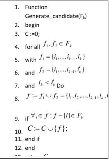
Function
Generate_candidate(F
k)
2.
begin
3.
C :=0;
4.
for all
f
1,
f
2
F
k5.
with
f
1
{
i
1,...,
i
k1,
i
k}
6.
and
f
2
{
i
1,...,
i
k1,
i
k
}
7.
and
i
k
i
k
Do
8.
f
:
f
1
f
2
{
i
1,
i
2,...,
i
k1,
i
k,
i
k
}
9.
if
i
f
:
f
{
i
}
F
k10.
C
:
C
{
f
};
11.
end if
12.
end
13.
return
C [image:33.595.65.256.66.395.2]14.
end
Figure 2.3 Apriori Algorithm
The subset function (line 5) finds the subset of candidate item sets contained in the current database transactional (t). Once these candidate item sets are identified from Cn, their supports are incremented (line 6-7). The algorithm terminates whenever there are no frequent item sets Fn in the nth iteration.
[image:33.595.65.253.474.749.2]33 To illustrate the discovery of frequent item sets in Apriori, consider Figure 2-5, which shows the steps of Apriori’s candidate generation described in Figure 2-4 on a database using a minsupp of 2. As shown in Figure 2-5, Apriori scans the database to find
candidate item sets of length 1, and from which it determines those that pass the support threshold (F1). In the second level, the algorithm generates candidate item set of size two 2 (C2) and scans the database to determine which subset of them is frequent (F2). The algorithm finally terminates after discovering frequent item sets of length three (F3). For the database shown in Figure 2-5, Apriori requires three passes over the
database in order to discover the complete set of frequent item sets.
Figure 2.5 :Apriori candidate generation example
2.4.2 Dynamic item-set counting
To speed up the discovery of frequent item sets in a database, a new ARM algorithm called Dynamic Item set Counting (DIC) was developed in Brin et al. (1997). DIC splits the database into several partitions marked by start points. Then, it calculates the supports of all item sets counted so far, dynamically adding new candidate item sets whenever their subsets are determined to be frequent, even if their subsets have not yet been seen at all transactions. The main difference between DIC and Apriori is that
whenever a candidate item set reaches the support during a particular scan, DIC starts
A C D B C E A B C E B E 10 20 30 40 Items Tid 2 3 3 1 3 {A} {B} {C} {D} {E} Support Itemset 2 3 3 3 {A} {B} {C} {E} Support Itemset {A B} {A C} {A E} {B C} {B E} {C E} Itemset 1 2 1 2 3 2 {A B} {A C} {A E} {B C} {B E} {C E} Support Itemset 2 2 3 2 {A C} {B C} {B E} {C E} Support Itemset 2 {B C E}
Support Itemset Scan DB C1 Scan DB C2 C3 Scan DB F1 F2 F3 C2 1 2 1 {A B C} {B C E} {A C E}
34 producing additional candidate item sets based on it, without waiting to complete the scan as Apriori does.
To accomplish the dynamic candidate item sets generation, DIC employs a prefix tree where each item counted so far is associated with a node. One of the drawbacks of DIC algorithm is its sensitivity to how homogeneous the data are. Particularly, if the
database to be mined is correlated, DIC cannot recognnise that an item set is frequent unless it has been seen in most transactions.
Experimental results using census and synthetic data sets (Agrawal and Srikant, 1994) indicated that DIC is faster by 30.00% than Apriori at a support threshold of 0.5% on the synthetic database. On the large and highly correlated census database, DIC outperformed Apriori at a support threshold of 36.00%. Both algorithms require a long period of training when the support is lowered, since the items in the census database occur frequently 95% of the time and thus yielding a very large number of candidate item sets.
2.4.3 Partition
An ARM approach that minimizes the I/O time by reducing the number of database scans to two has been proposed in Savasere et al. (1995). The algorithm divides the database into small partitions such that each partition can fit in the main memory and discovers frequent item sets locally using a stepwise approach, e.g. Apriori, in the first pass. A tid-list structure for each item set in a partition is then constructed. The tid-tid-list of an item set identifies rows in a partition that contain that item set. The cardinality of an item set tid-list divided by the total number of the transactions in a partition gives the support of that item set.
In the second pass, the algorithm performs union operations on local frequent item sets found in each partition to discover frequent item sets in the database as whole. One of the drawbacks of the partitioning algorithm is that it prefers a uniform data distribution in which, if the count of an item set is evenly distributed in each part, the vast majority of the item sets to be counted in the second pass are frequent. However, for an
35 A comparison of performance between Apriori and the partitioning algorithm using six market basket analysis data sets (Agrawal and Srikant, 1994) revealed that the
execution times of both algorithms increase when the support is reduced. A comparison using different number of partitions against the six benchmark problems indicates that the execution time decreases when fewer partitions are used, because the candidate set normally becomes smaller.
2.4.4 Frequent pattern growth
Apriori-like techniques use a candidate generation step to find frequent item sets during each iteration, and so these techniques require significant processing time and memory. Han et al. (2000) presented a new ARM approach, called FP-growth, that generates a highly condensed frequent pattern tree (FP-tree) representation of the transactional database. Each database transaction is represented in the tree by at most one path, and the length of each path is equal to the number of frequent items in the transaction representing that path. The FP-tree is a useful data representation because (1) all of the frequent item sets in each transaction of the original database are given by the FP-tree, and since there is a lot of sharing between frequent items, the FP-tree is smaller in size than the original database; and (2) the FP-tree construction requires only two database scans, whereby, in the first scan, frequent item sets along with their support in each transaction are produced, and in the second scan, the FP-tree is constructed.
Once the FP-tree is built, a pattern growth method is used to mine association rules by using patterns of length 1 in the FP-tree. For each frequent pattern, all possible other frequent patterns co-occurring with it in the FP-tree (using the pattern links) are generated and stored in a conditional FP-tree. The mining process is performed by concatenating the pattern with those produced from the conditional FP-tree. The mining process used by the FP-growth algorithm is not Apriori-like in that there is no candidate rule generation. One primary weakness of the FP-growth method is that there is no guarantee that the FP-tree will always fit in main memory, especially in cases where the mined database is dimensionally large.
36 (2010) compared matrix algorithm with FP growth algorithm using two case studies, the first one with 10000 items and 30000 transactions and the second with 30000 items and 30000 transactions. They concluded that the performances of the two algorithms are related to the characteristics of the given datasets and the minimum support threshold. Also, they concluded that the matrix algorithm performs better than the FP-Growth and their difference in the performance is more noticeable as the minimum support threshold decreases. For minimum threshold less than 10% the matrix algorithm is more efficient by up to 230%.
2.4.5 Confidence-based approach
Another possible solution to the problem of discarding rules with high confidence and low support, which abandons the support threshold and mines only top confidence rules, has been proposed (Li et al., 1999). Given a database, the end-user has to set an item set target, which represents the consequent of the desired outcome (rules). The problem of mining high confidence rules is to find all association rules where the target is the consequent. In doing that, the algorithm divides the problem of mining confidence rules into two steps. Step 1 involves splitting the original database into two sets, one set that holds transactions containing the target item set, T1, and the other holds the rest of the transactions, T2. The algorithm discards all items of the target from transactions in T1 and T2, therefore, the set of items in the original database I, becomes I = I – target. In the second step, all item sets, X, which appear in T1 but do not appear in T2 are
discovered, and rules such as
X
tg
, is produced, where tgis the target consequent. These item sets have a zero support in T2 but non-zero support in T1 and are called Jumping Emerging Patterns (JEP). The authors of (Li et al., 1999) have adopted two border methods from (Dong, 1999) to discover item sets whose support is zero in one sub-set, but non-zero in the other sub-set. The first border algorithm finds all item sets with non-zero support in a data set and names them horizontal borders. When taking two horizontal borders produced from two sets of data, as an input, the second border algorithm can derive all item sets whose support in one is zero, but non-zero in the other one.37
2.4.6 Matrix algorithm
In 2005, Yuan and Huang presented a novel algorithm for generation of association rules. The algorithm is called a matrix algorithm, and it creates a binary matrix with entries 0, 1 passing over the database only once creating a set of candidate items from which association rules are produced. The process of generating the matrix is the following: first the items in I are set as columns and the transactions D as rows in the matrix.
Let I={i1,i2,...,in} be the set of items and D = {t1,t2,...,tm} be the set of transactions. Then, the matrix G={gij} for i=1,...n and j=1,...m is generated using the following rule:
1,
0,
j i ij
j i
if i
t
g
if i
t
Using this generated matrix association rules are produced using the matrix algorithm: The 1-item set C1 consists of the sets which are subsets of single item in I , that is, C1 = {{i1},{i2},…,{in}}. In order to compute the support number for each set in C1, we express every set in C1 as a row vector in Rn, that is, we express {i1} as 1
1 {1, 0,..., 0}
S and {ik} as:
1 {0, 0,...,1,...0} k
S
where the kth element is 1 and others are 0. Then the support number of the set {ik} is calculated by:
11
,
m
k j k
j
supp
i
g S
Where <,> is the dot product of two row vectors and gj j=1,…,m are the rows of matrix G.
Then the set of all the frequent 1-item sets, L1, is generated from C1. If the support number of {ik} is beyond the user-specified support threshold Minsupport, that is,
k
supp i Minsupp
Then {ik}
L1 .The set of candidate 2-item sets C2 is the joint set of L1 with itself. Each subset in C2 consists of two items and has the form {ik, ij}, k < j. Similarly, we specify each set in C2 a row vector in Rn. For example, for the set {ik, ij}, the specified vector is:
2
, {0,..., 0, 0,1,..., 0, 0,1,..., 0}
k j
S
Where the kth and jth elements are 1 and others are 0. The support number of the set {ik, ij} is :
2,1
,
int
2
m
38 where int[・] is the integrating function that changes a real number to integer by
discarding the number after decimal point.
The frequent item set L2 is generated from C2 with the set whose support number is beyond the user specified support threshold Minsupport, that is:
k,
j
supp
i i
Minsupp
then {ik, ij} ∈ L2.
After the frequent 2-item sets L2 is obtained, it can be used to generate C3.
The process is repeated with successively increasing number k until either Ck or Lk is empty, where each subset in Ck has the form {il1, il2 , ・・・ , ilk}
including k items, and is generated from the frequent (k − 1)−item sets Lk−1, and Lk is the frequent k−item sets generated from Ck with the set whose support number is beyond the user specified threshold.
At the end of procedure, we can get the all frequent item sets by the following formula. Let the procedure is terminated after step k, then:
1
1
k i i
L
L
2.4.7 Multiple supports Apriori
The support constraint is the most important factor that controls the number of association rules produced (Agrawal et al., 1993; Bayardo and Agrawal, 1999; Zaki, 2000). Almost all current ARM algorithms use a single support, but setting the support to a high value results in disposal of some useful, rare items in the database. Furthermore, to capture such rare items, one has to set the support to a very small value, which can lead to the generation of many useless rules (Liu et al., 1999, Li et al., 1999).
To overcome such a problem, Liu et al. (1999) proposed a multiple-support Apriori-like approach, called MSapriori, which assigns different support values for each item in the database. This enables users to express different support requirements for different rules. The support for a particular rule in MSapriori is the lowest minsupp value among the items in that rule. The candidate generation step in MSapriori is similar to the generate function in the Apriori algorithm.
39 Apriori. However, the execution time spent to find frequent item sets for both algorithms is roughly the same.
2.4.8 Hash-based technique and pruning
Generally, the computational cost of ARM is largely determined by the speed of the discovery of frequent one- and two-item sets. Empirical results from Agrawal and Srikant (1994) suggest that the computational cost in the initial iterations dominates most of the execution time for the candidate generation phase. When the number of frequent item sets during iteration 1 is large, the expected number of candidate item sets at iteration 2 is also large, and so reducing the size of the candidate item sets in the early iterations may result in huge savings in processing time and memory. A hash-based technique, called Direct Hashing and Pruning (DHP), has been proposed in Park et al. (1995) to efficiently reduce the size of candidate item sets in early iterations.
DHP works as follows. While scanning the database to find frequent one-item sets, a hash tree, H1, is built for candidate one-item sets to facilitate the search. The algorithm evaluates during the scan whether an item exists in the hash table, and if so, the count of the item is incremented by 1; otherwise, the item is inserted into the hash table and is given a count of 1. Also, when the occurrences of all one-item sets are counted for each transaction, all two-item sets are produced and hashed into another hash table, H2, where a count is initialized to 1 for each item set. Once the database is scanned, we can obtain the possible candidate two-item sets from H2.
Pruning occurs to reduce the database size during the scan in which not only a transaction is trimmed but also some of the transactions are removed. DHP trims an item in a transaction t if it does not have a certain number of occurrences in t’s candidate item sets. For example, If the support is set to 2, t = XYZWP and four two-subsets, (XZ, XW, XP, WP), exist in the hash tree constructed for candidate two-item sets, H2, the number of frequencies according to each item in t is 3, 0, 1, 2, 2, respectively. For frequent three-item sets, only three items in t, e.g. (X, W, P), have occurrences above the support threshold. Consequently, these three items are kept in t and items Y and Z are removed.
Empirical studies indicate that DHP reduces the execution times not only in the second iteration, when the hash table is employed by DHP to facilitate the production of
40 magnitude smaller than that of Apriori, but the execution time of DHP is slightly larger than that of Apriori in the first iteration, owing to time required for building the hash table for candidate two-item sets.
2.4.9 Eclat algorithm
To minimize the number of passes over the input database, the Eclat algorithm was presented in Zaki et al. (1997). It requires only one database scan, thus addressing the question of whether all frequent item sets can be derived in a single pass. Eclat uses a vertical database transaction layout, where frequent item sets are obtained by applying simple tid-list intersections, without the need for complex data structures.
A recent variation of the Eclat algorithm, called dEclat, has been proposed in (Zaki and Gouda, 2003). The dEclat algorithm uses a new vertical layout representation approach called a diffset, which only stores the differences in the transactions identifiers (tids) of a candidate item set from its generating frequent item sets. This considerably reduces the size of the memory required to store the tids. The diffset approach avoids storing the complete tids of each item set; rather the difference between the class and its member item sets are stored. Two item sets share the same class if they share a common prefix. A class represents items that the prefix can be extended with to obtain new class. For instance, for a class of item sets with prefix x, [x] = {a1, a2, a3, a4}, one can perform the intersection of xai with all xaj with j>i to get the new classes. From [x], we can obtain classes [xa1] = {a2, a3, a4}, [xa2] = {a3, a4}, [xa3] = {a4}.
Experimental results on real world data and synthetic data (Zaki and Gouda, 2003) revealed that dEclat and other vertical techniques like Eclat usually outperform horizontal algorithms like Apriori and FP-growth with regards to processing time and memory usage. Furthermore, dEclat outperforms Eclat on