The London School of Economics and Political Science
Rational Bubble, Short-dated Volatility Forecasting and
Extract More from The Volatility Surface
Yiyi Wang
Declaration
I certify that the thesis I have presented for examination for the PhD degree of the London School of Economics and Political Science is solely my own work other than where I have clearly indicated that it is the work of others (in which case the extent of any work carried out jointly by me and any other person is clearly identified in it).
The copyright of this thesis rests with the author. Quotation from it is permitted, provided that full acknowledgement is made. This thesis may not be reproduced without the prior written consent of the author.
Abstract
The thesis covers three main chapters. The first chapter (which is a joint work) we develop a theoretical model of rational bubble. In equilibrium, a bubble can persist until it bursts following an exogenous shock, even when all the agents are aware of the bubble and that it will burst in finite time. Applying the model in the context of the sub-prime mortgage crisis, we argue that excessive sub-prime lending behaviour may be sensible with the introduction of securitization. W e thus provide a rational explanation for the housing bubble and the dramatic increase in sub-prime default rates.
In the second chapter I conduct empirical short-dated volatility forecasting in foreign exchange, and carry out a realistic volatility swap trading strategy based on the forecast. Additional to applying regime-switch technique, I propose a double-step approach to circumvent the disadvantage of employing GARCH-type model in the high frequency data in FX market, so that it can separate the effect of intraday/intraweek seasonality and pre-scheduled macroeconomic data releases from the underlying data process. By keeping a battery of models and rotating among them, the forecast ability gets significantly enhanced and the trading profit is pronounced even after considering transaction cost.
Acknowledgements
Table of Contents
Chapter 1 A Rational Bubble Model and Application in Sub-prime Mortgage Crisis... 1
Abstract... 1
1. Introduction... 2
2. Related L iterature... 4
3. Baseline M o d e l...5
3.1 Basic Setup... 6
3.2 Characterization of Equilibrium... ... 6
3.3 Proof of Equilibrium... 7
3.4 Extension... 10
3.5 Summary... 12
4. Application in Sub-prim Mortgage M a rk e t...13
4.1 Basic Setup... 14
4.2 Concept of Bubble... 15
4.3 Securitization...16
4.4 Implications...17
5. Conclusion ... 18
References... ...20
A Technical Appendix... 21
A .l Proof of the necessity of exogenous shock in baseline m odel... 21
A.2 Proof of Lemma 3 .1 ... 24
A.3 Proof of Lemma 3 .2 ... ...34
A.4 Proof of Proposition 3.2... 35
A.5 Specification of wealth and income in the model of sub-prime mortgages...36
A.6 Proof of Proposition 4.1... 37
A.7 Proof of Proposition 4 .2 ... 38
Chapter 2 Short-dated Volatility Forecasting... 41
Abstract...41
1. Introduction... 42
3. Data and Methodology... 46
3.1 D ata...46
3.2 Methodology...48
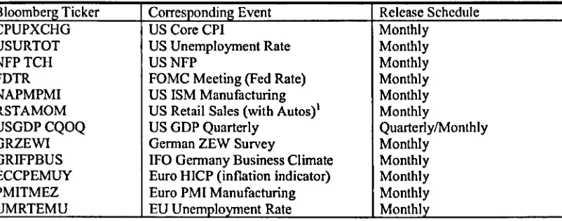
3.2.1 Seasonality and Event... 48
3.2.2 Forecasting Models ... 50
4. Empirical Results...53
4.1 Seasonality and Event Adjustment... 53
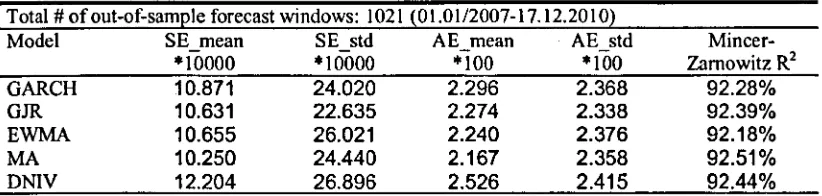
4.2 Forecast Results... 54
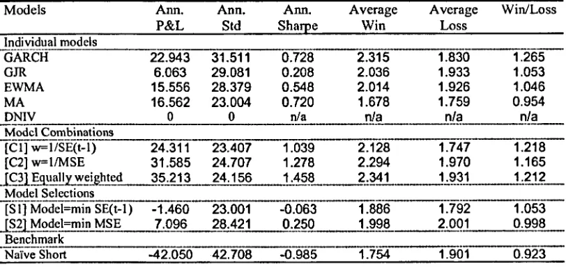
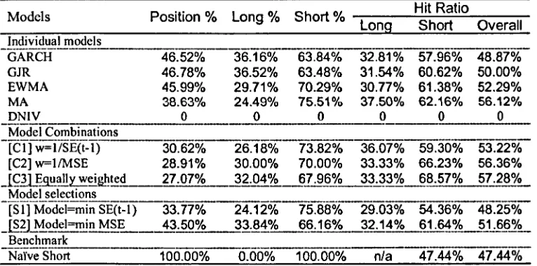
4.3 Trading Strategy... 56
5. Robustness check...61
5.1 Daily Data... 61
5.2 No Seasonality or Event Adjustments...61
5.3 Lagged Realized Volatility... 62
5.4 Fixed-parameter EW M A... 62
5.5 Realized Volatility Calculated in Hourly Data... 62
6. Conclusion ... 63
A Appendix: Steady-state Probabilities for Markov Chain... 65
References...66
Tables... 71
Table 1. General Statistics for Hourly Return and Variance... 71
Table 2. Macroeconomic Data Releases... 71
Table 3. Statistics of Delta-neutral IV and Model-free IV from Oct 2008-Dec 2010...72
Table 4. Event Effect (£¿1... 72
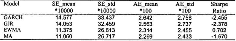
Table 5. Squared Error and Absolute Error (RV from Daily Data)... 73
Table 6. Model Combination and Model Selection... 73
Table 7. Annual Performance, Average Win and Loss... 74
Table 8. Long/Short Position and Hit Ratio of a Volatility S w ap ...75
Table 9. Maximum Draw dow ns... 76
Table 10. Annual Performance of Volatility Swap of Model Combinations... 77
Table 11. Sharpe Ratio Comparison... 77
Table 12. Model Performance from Daily D a ta ...78
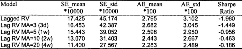
Table 14. Performance of Lagged Realized Volatility and Its Moving Averages... 79
Table 15. Performance of fixed-parameter EWMA ... 79
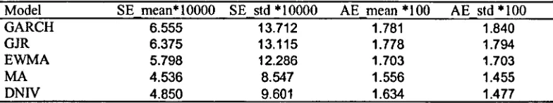
Table 16. Squared Error and Absolute Error (RV from Hourly D ata)... 80
Table 17. Squared Error and Absolute Error (RV from Hourly Data) without Seasonality or Event Adjustm ents... 80
Figures...81
Figure 1. Hourly Return and V arian ce... 81
Figure 2. Model-free and Delta-neutral Implied Volatility (2w window, annualized)... 81
Figure 3. Comparison of Variance Autocorrelation before and after A djustm ent... 82
Figure 4. Intraweek Seasonality (Sh) ...82
Figure 5. Annualized 2-Week Realized Volatility (Daily Frequency)... 83
Figure 6. Cumulative P&L of Single Models and Naive S h o rt... 84
Figure 7. Cumulative P&L of Model Combinations...85
Figure 8. Annualized 2-Week Realized Volatility (Hourly Frequency)... 86
Chapter 3 Extract M ore from The Volatility Surface... 87
Abstract...87
1. Introduction...88
2. Data, Key Variables and Hypotheses...92
2.1 Data Source... 92
2.2 Key Variables...93
2.3 Hypotheses... 95
3. Empirical Results...95
3.1 Fama-Macbeth Regression... 96
3.2 Portfolio Trading Strategy... 99
3.2.1 Single S o r t... 99
3.2.2 Double Sort ... 100
4. Information Proxies... 101
5. Example: Merger and Acquisitions ... 104
6. Conclusion ... 106
References...107
Table 2. Fama-MacBeth Regression on Weekly Return ...112
Table 3. Fama-MacBeth Regression on Weekly A lp h a ... 113
Table 4. Fama-MacBeth Regression of Multiple Horizons ... 114
Table 5. Portfolio Trading Strategy (Single Sort on SKEW)... 115
Table 6. Portfolio Trading Strategy (Single Sort on TERM)... 116
Table 7. Effect of TERM in the Lowest and Highest SKEW Quintiles... 117
Table 8. Effect of SKEW in the Lowest and Highest TERM Quintiles... 117
Table 9. Panel Regression of Information Proxies ... 118
Table 10. PIN in Double Sorting on SKEW and T E R M ...119
Table 11. Fama-MacBeth Regression after Including Information Proxy... ...120
Table 12. Takeover Distribution in SKEW-TERM Portfolios... 121
Charts...122
A Rational Bubbles Model and
Application In Sub-prime Mortgage Crisis
Zijun Liu
London School o f Economics
Y iyi W ang
London School of Economics
N ovem ber 27, 2011
A bstract
W e develop a theoretical m od el o f rational bu bble. In equilibrium , a bu bb le can persist until it bu rsts follow ing an exogen ous shock, even when all the agents are aware o f the b u b b le and that it will burst in finite tim e. A p p lyin g the m odel in th e context o f th e recent su b-prim e m ortgage crisis, we argue that excessive sub-prim e lending behavior m ay b e rational w ith th e in trodu ction o f securitization. T h e process is much like a Ponzi schem e w here lending is profitable as long as investors continue to invest, and v ice versa. W e thus provide a rational explanation for the housing bu b b le an d the dram atic increase in su b-prim e default rates.
1
Introduction
Bubbles have been the central theme of the financial market in the past decade. Following the burst
o f the dot-com bubble in 2001, there have been strong deviations o f asset prices from fundamentals
across many different markets and countries, such as the US housing bubble, the Chinese stock
market bubble, the worldwide commodity bubble, and so on. Especially, the collapse of the US
housing bubble and the sub-prime mortgage market has eventually lead to the recent global financial
crisis.
However, the existence o f bubbles still remains theoretically controversial. For example, the
backward induction argument and the transversality condition preclude the existence o f bubbles
in finite-horizon models and infinite-horizon inter-temporal models respectively. Moreover, the
efficient market hypothesis implies that the presence o f sufficiently many well-informed arbitrageurs
will ensure that large deviations from fundamental values are not possible. Nonetheless, Abreu and
Brunnermeier (2003) showed that bubbles can persist given dispersion o f opinion among rational
arbitrageurs and the presence o f behavioral traders. Hence the backward induction argument could
fail if agents do not have common knowledge about the timing o f the burst o f the bubble.
We develop a theoretical model o f bubbles and argue that speculative bubbles can be sustained
even if all agents are rational. Our result relies on the assumption that the bubble will burst
following an exogenous shock and agents are only partially informed o f the timing o f this shock. In
our model, the investors are fully aware that the asset price has departed from fundamentals since
the start o f the bubble, therefore they only have incentives to buy the asset if they expect to sell the
asset later at a high price. Ideally each investor would like to sell the asset just before the bubble
bursts in order to maximize profits. Because investors have heterogeneous beliefs about the time of
the burst, they would have different exit strategies, hence the backward induction argument does
not apply. This intuition is very similar to Abreu and Brunnermeier (2003), however our model is
different in several ways. Most importantly, there is no behavioral traders in our model, and agents
are fully rational in the sense that they are well aware o f the bubble since the very beginning rather
than being sequentially informed o f the mis-pricing.
Our model is a very simplified illustration of the above intuition. In the baseline model, there
are two investors who can trade one virtually worthless asset in each period. Each investor needs
to pay a fixed premium above the market price when he wants to buy the asset from the other.
The process will terminate following an exogenous shock taking place at an unknown date. Each
investor will receive a noisy signal o f this date but does not know the signal of the other. That is,
the investors have heterogeneous beliefs about the date when the bubble will burst. The uncertain
timing o f the burst o f the bubble together with heterogeneous beliefs ensure that the model does
In equilibrium, the investors will ride the bubble until some point according to their own exit
strategy which depends on their private beliefs. Although this is a zero-sum game, each investor
has the incentives to ride the bubble as far as he could, because the potential gain from winning
the game is increasing as the bubble grows. The intuition is that, no matter how large the bubble
is, there is always a good chance that my opponent will exit after me in which case I will make a
larger profit. Thus the investors would gamble for profits while being perfectly aware o f the bubble.
Moreover, we extend the model with noisier signals and different strategies o f the investors. We
show that bubbles tend to last longer in illiquid markets.
We then apply the model in the context o f the recent housing bubble and sub-prime crisis in
the US in order to derive more economic implications. Although the results o f the model can be
naturally extended to many speculative bubbles we have experienced in the financial market, our
application o f the model in the sub-prime mortgage market is not a straightforward extension. In
particular, the housing bubble in our model is not supported directly by speculative buyers but
through excessive lending and securitization behavior o f the mortgage lenders.
The sub-prime mortgage industry has been partly blamed for the emergence and collapse of
the recent US housing bubble. Loose lending standards have provided excessive credit to the sub
prime borrowers who have a poor credit history and ability to repay their loans. It has been argued
that, as a result of the fact that the sub-prime mortgage lenders securitize their loans and sell the
securitized products to the investors, the lenders have shifted the risks associated with sub-prime
lending away and do not have enough incentives to maintain the quality o f the borrowers, hence we
observe the boom and collapse of the sub-prime industry. The dramatic increase in the default rates
in the industry after the housing bubble burst might suggest that investors have underestimated
the risk inherent in the mortgage-backed assets that they bought. However, this cannot stand if
we assume that the investors are rational and anticipate the moral hazard issues ex-ante.
Our paper tries to establish a different perspective by extending our model o f rational bubbles.
Because sub-prime borrowers frequently incur difficulties to repay, the payoff from lending largely
depends on the price o f the houses that will be repossessed by the lenders in case o f default. If
house prices always rise, there would be virtually no risk associated with lending. House prices
would keep rising if the lenders can fuel the demand by keeping lending generously to the borrowers
and refinancing existing borrowers with financial problems. Thus sub-prime lending would become
profitable and rational with rising house prices, or a housing bubble.
House prices cannot rise forever. When the bank stops lending following a liquidity shock1, the
housing bubble will burst and house prices will plummet due to foreclosures on sub-prime loads
accumulated over the years. Thus sub-prime lending would become unprofitable before the burst
o f the housing bubble and the bank would not lend in the very first place by backward induction.
However, the introduction o f securitization would enable the bank to transfer the risk to investors
and gamble in the same way as in the baseline model. That is, banks have incentives to lend as long
as investors are willing to buy the mortgage-backed securities (MBS), and investors have incentives
to buy the MBS as long as banks are willing to refinance borrowers. Because o f the uncertain
timing of the shock, a bubble in the house price can persist with the same intuition in the baseline
model.
The rest o f the paper is organized as follows. Section 2 is a brief literature review. Section
3 introduces the baseline model as well as some extensions and implications. Section 4 describes
and discusses the application of the model in the sub-prime mortgage market. Finally Section 5
concludes.
2
Related Literature
Allen et al. (1993) provided necessary conditions for a bubble to occur. They say that a rational
expectations equilibrium exhibits a strong bubble if the price is higher than the dividend with
probability one. They show that in a finite-period general equilibrium model in which a bubble
is possible, each agent must have private information in the period and state in which the bubble
occurs, and the agents’ trades cannot be common knowledge. Allen and Gorton (1993) show that a
bubble can exist because the fund managers without private information will churn at the expense
o f uninformed investors, who cannot observe the skill o f the fund managers. These papers assume
that all agents are fully rational.
Abreu and Brunnermeier (2003) developed a model of bubbles in which rational arbitrageurs
interact with boundedly rational behavioral traders. They show that the inability o f arbitrageurs
to temporarily coordinate their selling strategies together with the presence o f behavioral traders
results in the persistence o f bubbles over a substantial period. In Abreu and Brunnermeier (2003),
arbitrageurs sequentially become aware o f the bubble and hence are uncertain about the timing
o f the burst o f the bubble. The incentives of the arbitrageurs to time their exits as close to the
burst o f the bubble as possible lead to the persistence o f the bubble. Sato (2008) extended the
paper and show that the presence o f relative ranking tournament among fund managers affects
their incentives to attack or instead ride asset bubbles.
Our model is different from the above in the following ways. All agents are fully rational in our
model. The bubble will end in finite time with probability one, but the length o f the bubble is not
period and state in which the bubble occurs, but the time at which the bubble will burst. That
is, all agents are fully aware o f the bubble from the beginning, but they do not know each other’s
beliefs about the timing o f the burst o f the bubble. Moreover, the agents’ trades are common
knowledge and there is no sequential awareness.
On the application in the sub-prime mortgage market and securitization, there is a rich literature
focusing on the role and implication o f securitization. It remains controversial whether lenders
exploit asymmetric information to sell riskier loans into the public markets or retain riskier loans
in response to regulatory capital incentives (regulatory capital arbitrage). Calem and LaCour-Little
(2004) argue that, for most mortgage loans, existing regulatory capital levels are too high, creating
an incentive to securitize the least risky loans. In addition to regulatory capital rules favoring
securitization, the presence o f information asymmetries also encourages securitization. DeMarzo
and Duffie (1999) using a liquidity based model o f securitization show that if the issuer does not
wish to retain any portion o f the mortgage backed security, then she should sell only those loans
having the lowest degree o f asymmetric information into the pool and retain those loans with high
degree of asymmetric information.
Our paper innovates in arguing that securitization enabled the bank to gamble with the investors
and benefit from lending excessively to sub-prime borrowers and riding the bubble. This result is
consistent with Keys et al. (2008) who empirically examine the default probability o f portfolios
with different securitization levels and find that portfolios with higher securitization volume are
like to have high default rates, hence implying that the bank may have incentives to loosen lending
standard in presence o f securitization. Furthermore, Coval et al. (2007) show that many structured
finance instruments can be characterized as economic catastrophe bonds that default only under
severe economic conditions. This is consistent with our model in which the MBS would only have
a negative return when the bubble bursts with a small probability. The difference is that Coval
et al. (2007) blame the rating agencies for the mis-pricing of these instruments whereas we show
that a bubble can persist without such intermediation problems.
3
Baseline Model
Using a parsimonious model, we will show that rational agents with heterogeneous beliefs will ride
the bubble and gamble on future profits given high enough incentives. The model is very simple
but illustrate the intuition why rational investors would speculate on over-priced assets. The basic
3.1
Basic Setup
Consider a discrete-time model with infinite time periods 0,1,2... Suppose there are two investors:
investor A and investor B, each with an initial wealth of IVo- They will both receive income in each
period2. The amount o f income they receive in period t is fce.
There is an asset that has a fundamental value o f 1 and can be traded between the two investors.
Assume that the asset can only be bought at a multiple k of its current price3. So in period t, one
investor can decide whether or not to buy this asset from the other at a price o f k*.
The above assumption is important because it provides incentives for the investors to ride the
bubble. We can think o f it as price impact o f trades in the reality.
Suppose that both investors will experience a liquidity shock at a random date T and they
will consume all their wealth at this date (the asset itself has a consumption value o f 1). Both
investors will maximize the expected value of this consumption, which we denote by C. Assume
that investors are risk-neutral and have zero discount rate. Hence the expected utility of each
investor is the expectation o f his final consumption at the date of liquidity shock.
Finally we denote the date of liquidity shock by T and assume that it will be drawn ex-ante from
a Geometric distribution4 with parameter p. Each investor will receive a noisy signal s about T.
The signal can be T — 1 or T-h 1 with probability 1 respectively5. This assumption o f heterogeneous
beliefs was necessary for a bubble equilibrium 6 to exist (see Appendix A .l for a detailed proof).
3.2
Characterization of Equilibrium
P r o p o s it io n 3 .1 . Given the above assumptions, there exists a Nash equilibrium such that each
investor buys the asset until their signaled date, i.e. if an investor received a signal s, he will buy
the asset at period t if and only if t < s.
aThis is to ensure that they have enough funds to sustain the bubble in the long run. That is, we need the investors to have finite capital but not be constrained by capital in the long run. Alternatively, we can assume that they have unlimited access to short-term financing.
3Here we show that a particular bubble price path with a constant inflator is possible given certain parametric restrictions. Any other price paths with time-dependent inflator are possible as long as those restrictions are satisfied.
4We need distributions with probability densities that do not converge to zero too fast along the tails. For example, Poisson distribution will not work. The intuition is that, when the random variable is Poisson distributed, if one agent received a sufficiently large signal, it will be extremely unlikely that other agents had larger signals. Other distributions that will work in our model include discrete uniform distribution and logarithmic series distribution.
®Note that the investors are correct on average. There are good reasons why investors in reality would have dispersed opinions the timing o f an exogenous event, such as information cost. W e have adopted the simplest possible noise distribution here, which can be extended as we show later.
The following table illustrates the wealth o f the investors and the asset price (that one investor
needs to pay to buy it from the other) in equilibrium before the bubble bursts:
Date 0 1 2
Income N /A k ki2
Wealth o f A * W0 W o + k + k * W0 + k + k2 + k - k 2 . . .
Wealth o f B W0 * W0 + k - k W o + k + k 2 - k + k2 . . .
Asset Price 1 k k2
The asterisk indicates the ownership o f the asset. A t the date of liquidity shock, the investor
will consume all his available wealth and the asset (if he owns it).
The investors are subject to the budget constraint that Wj > 0 for all t. We can see from the
above that this constraint is always satisfied.
3.3
Proof of Equilibrium
Let’s check the incentives o f the investors in each period given that the asset is still being traded.
Suppose that investor A received a signal s (and that he can buy the asset at period s, s —2, s —4 , ...) .
Denote his wealth at period t by
Wt-At period s, investor A knows for sure that T — s + 1 given a signal s. So he will not buy the
asset since he cannot sell it at a higher price in the future.
At period s —2, if investor A buys the asset at price fc*- 2 , he will lose if T = s — 1 with probability
P ( T = s — l|s) = and he will gain if T = s + 1 with probability P ( T = s + l|s) = 1|1^_p)3 •
5 + 1 Ea- 2(C|s,buy) = I 1
f \W.-3 + { k -
1)k*~*
+ X **1^ t = s —1
+ 1
l + ( l - i>)2[w v-2 + i - * * ~ a + * - 1]
If investor A does not buy at s — 2, his expected final consumption is
5 + 1
E s_ 2(C|s, don’t buy) = + X **1
1
l + ( l - p)2[W +2 + f c - 1]
Hence we see that investor A would prefer buying when
E a_ 2(C|s,buy) - E a_ 2(C'|s, don’t buy)
> 0
This holds for every s if and only if
k > 1 + 1
( 1 - p ) 2 (3.1)
At period s — 4, investor A knows that investor B will always buy the asset in the next period,
so it is optimal for investor A to buy. This is true for all the remaining periods.
Now we go on to check the incentive o f investor B given that his counterpart follows the
equilibrium strategy. Suppose that investor B received a signal s (and that he can buy the asset
at period s + 1, s — 1, s — 3 , . . . ) .
At period s + 1, the liquidity shock will happen and there will be no trading at this period.
At period s — 1, since there was no shock taking place at s — 1, investor B knows for sure
and quits at s, with probability |; and he will gain if investor A gets signal s + 2 and continues to
buy at s, with probability 5, too. Thus the expected final consumption from buying is
Ea_ 1(C|«,buy) = i [ W . - i + (k — l ) * - 1 + h* + ks+1}
+ h w„ - 1 + 1 - k *-1 4- ks + Jts+1]
If investor B does not buy at s — 1, his expected final consumption is
E ,_ x(C|a>don’t buy) = \[Wa- i + Jb* + ks+l]
+ ^ [ W , - i + A:s + fcs+1]
Hence we see that investor B would prefer buying when
E^-iiC Is, buy) - E
5
_i(C |s, don’t buy)= |[(fc - l)*—1] + |[1 - fc*-1]
> 0
This holds for every s if and only if
Jfc > 2 (3.2)
At period s — 3, if investor B buys the asset at the price ks~3, he will lose if investor A gets
signal 5 — 2 and quits the market then, with probability 2[1+J _ ?)p j; otherwise investor B will gain
E s_ 3( C h b u y ) = — ^ (i[W V .3 + 1 - k°~3 + k3~2 + k - 1)
+ \ [W a- 3 + ( k - 1 )ka~3 + k3~2 + k3- 1})
(1 — p)^
+ r V _i .g _ . E a- 1(C|s,buy)
The expected final consumption if investor B does not buy at s — 3 is
E s_3(C|s,don’t buy) =
1 + (1 - p) 2
(1 - p ) 2 «+1
+r ^ i - . - 3 + E / * i
which is less than E s_3(C|s,buy) given that condition (3.2) holds.
At all the remaining periods, investor B will always buy since he knows that investor A will not
quit in the next period.
Therefore, the above is a Nash equilibrium if both conditions (3.1) and (3.2) are satisfied. Since
2 < 1 + -(j-jp ) ? , the equilibrium holds if and only if
‘ > ‘ + ( 5 ^ # <3 -3 >
Hence we have derived a condition for which the bubble can persist in equilibrium. That is,
given a high enough reward, rational agents with heterogeneous beliefs have incentives to ride the
bubble, even though they know en-ante that this is a bubble and it will burst in finite time.
3.4
Extension
In the following we will extend the model to show that a bubble equilibrium holds with noisier
signals and different strategies o f the investors. In particular, there exists a Nash equilibrium in
which the investors buy until some period before or after their signals, for different ranges o f the
The extended model will be the same as the baseline model in that the exogenous shock will
happen at time T which follows a Geometric distribution with parameter p. The difference is that
now each investor will receive ex-ante a signal s which is uniformly distributed over the interval
[m ax{0,T — n },T + n].
We will show that there exists a set o f Nash equilibrium characterized by their equilibrium
strategies and conditions on the price multiplier k. In each equilibrium N E m where m is an
integer, an investor with private signal s buys the asset at period t if and only if t < s + m, for a
certain interval o f k.
L em m a 3 .1 . Suppose that investor B has a signal s' and will buy the asset at t with t < s’ + m.
Then if it is optimal for investor A to buy at time t, it is also optimal for him to buy at any time
i < t.
Proof. See Appendix A .2
□
Lemma 3.1 can be interpreted as that if the value o f k is a large enough incentive for the investor
to buy at time t, then it is also sufficiently large for the investor to buy at any time before t, given
that his counterpart follows the euqilibrium strategy. In other words, the necessary condition on k
for the investor to buy at time t is weakly increasing in t.
L em m a 3.2. Let g(m ,n,p) be a function such that
g(m ,n,p) = <
m + n + j + I / , _ \ j , _ 2 n _ M _ - O r 2 -> j= l m +n+j+3 v1 P> + 2 n + l 'i Pi
'2r
*3-E 5 o ( i - p ) i
I X ^ & t t - p y + a g i U - p ) *
— if m > —n — 1 1—1
if m < —n — 1
where m is an integer, n is a non-negative integer and p is a probability. Then g is an increasing
function of m and is greater than 1.
Proof. See Appendix A.3 □
P r o p o s itio n 3.2 . Given that g(m, n ,p) < k < g (m + l ,n ,p ) , there exists a Nash equilibrium N E m
such that each investor with a private signal s will buy the asset at t if and only i f t < s + m where
m < n — 2.
We can see that g(m ,n,p) is independent of m when m < —n — 1, and then increasing with
m. In other words, when the equilibrium strategy is to exit very early, we have a threshold level
of incentive k that must be satisfied to make the investors trade. Otherwise, a larger m leads to a
higher lower-bound o f k, i.e. in order to encourage the investors to exit the market relatively late
and ride the bubble for a longer period o f time, a higher incentive is needed. Hence the implication
is that bubbles tend to last longer in markets with higher market impacts o f trade. On the other
hand, a smaller incentive is required with more conservative exit strategies adopted by the investors.
In addition, g(m>n,p) is decreasing with n and increasing with p. The intuition is that the
less accurate the signals, the more likely that someone will exit after myself, and hence a small
incentive is required to encourage people to trade. Similarly, the less likely that the exogenous
shock happens in the next period, the more willingness-to-trade the investors have. An extreme
case is when n = 0 and g(m ,n ,p) —► oo. This is intuitive since when every investor knows definitely
when the shock will happen, backward induction eliminates the bubble ex-ante.
This game is not constrained to be played only between two investors. Since the one who sells at
time t and buys at time t + 2 is not necessarily the same person, it is straightforward to extend the
result to more investors, assuming that the investors cannot observe who have exited the market.
Otherwise, the investors would update their beliefs upon observation and the model will become
more complicated. We leave it to future research.
3.5
Summary
To summarize, we have developed a model o f rational bubbles based on several assumptions. Firstly,
we have assumed that the asset price needs to be inflated by an exogenous factor every time being
traded. Secondly, the bubble will burst following an exogenous shock and the date o f the shock
follows a Geometric distribution. Thirdly, the investors have heterogeneous beliefs about the date
of the shock.
Our model shows that an equilibrium in which a bubble can persistently exists given that the
bubble grows fast enough. In the baseline model, the speed at which the bubble grows only depends
on k, the exogenous inflation factor, hence the implication is that bubbles are more likely in illiquid
markets where trading impact on the market price is relatively high. In the extension we have
shown that a higher inflation factor will result in bubbles that last longer. Furthermore, a higher
dispersion o f signals and a smaller probability o f exogenous shock could also extend the life o f the
bubble.
Our model does not have a realistic background and aims at illustrating the intuition. However,
section we will apply the model in the context o f the recent US housing bubble and sub-prime
mortgage crisis. Note that this is not a straightforward extension. In particular, the housing
bubble in our model is not supported directly by speculative buyers but through excessive lending
and securitization behavior o f the mortgage lenders. One o f our objectives in doing so is to show
that the intuition can be applied in more sophisticated frameworks.
4
Application in Sub-prime Mortgage Market
The sub-prime mortgage industry has been partly blamed for the emergence and collapse o f the
recent US housing bubble. Loose lending standards have provided excessive credit to the sub
prime borrowers who have a poor credit history and ability to repay their loans. It has been argued
that, as a result o f the fact that the sub-prime mortgage lenders securitize their loans and sell the
securitized products to the investors, the lenders have shifted the risks associated with sub-prime
lending away and do not have enough incentives to maintain the quality o f the borrowers, hence we
observe the boom and collapse of the sub-prime industry. The dramatic increase in the default rates
in the industry after the housing bubble burst might suggest that investors have underestimated
the risk inherent in the mortgage-backed assets that they bought. However, this cannot stand if
we assume that the investors are rational and anticipate the moral hazard issues ex-ante.
We try to establish a different perspective by extending our model o f rational bubbles. We argue
that the introduction o f securitization would enable the bank to transfer the risk to investors and
gamble in the same way as in the baseline model. That is, banks have incentives to lend as long as
investors are willing to buy the mortgage-backed securities (MBS), and investors have incentives to
buy the MBS as long as banks are willing to refinance borrowers. Because o f the uncertain timing
of the shock, a bubble in the house price can persist with the same intuition in the baseline model.
The sub-prime mortgage market is a complex mechanism involving the processes o f mortgage
lending, securitization and derivatives trading with many individual investors and financial inter
mediates and a variety o f practices and contractual terms. In order to illustrate our ideas with as
few unnecessary complications as possible, our model is a much simplified version o f the real world.
In particular, the mortgages have a simple structure and will last for one period only. Moreover,
house prices will stay constant at a “bubble” level rather than continuously increasing. These are
simplifications to better deliver the intuition rather than necessary consequences or constraints of
4.1
Basic Setup
Our model is set in infinite discrete time periods with t = 1 ,2 ,3 ,___ There are three classes of
agents: borrowers, a bank and an investor. All agents are risk neutral.
As we will see later, the setup of the model is in essence the same as the rational bubbles model
we introduced in the previous section. In particular, the bubble process will terminate following an
exogenous shock, and the bank and the investor maximize their terminal wealth (or consumption).
Therefore, we will need to assume an initial wealth and a deterministic income process for the
bank and the investor so that the capital constraints are satisfied7 For the purpose o f simplicity,
we omit the details o f these assumptions here (See Appendix A.5 for full specification). Similarly,
we assume that all agents apart from the borrowers are subject to a liquidity shock and they will
behave strategically to maximize consumption at the date o f the shock as in the baseline model8.
4.1.1 Borrowers
In each period, there will be N new sub-prime borrowers who would like to gain access to the
housing market. Each new borrower has zero initial wealth and expects to receive an income I in
each period. The borrowers are called “sub-prime” because their income is very unstable, that is,
their income is subject to a shock with probability A. After an income shock, the borrower will not
receive any income for the current and all remaining periods. Assume that the borrowers realize a
large enough utility from living in a house so that they always want to borrow.
4.1.2 Mortgage Lender
There is a bank (or mortgage lender) who has the ability to identify the borrowers and lend them
money through issuing mortgages. We assume that the length o f the mortgage is one period and the
mortgage interest rate is exogenously given by r. That is, after one period, the mortgage borrowers
must repay 1 + r times the amount o f the loan. Assume that the borrowers will be able to repay
the loan fully with an income o f I.
The mortgage contract also stipulates that the bank has the right to repossess the borrowers’
homes should they default. The bank will immediately liquidate the repossessed houses for cash.
The bank can refinance mortgages, i.e. it can lend to the borrowers with existing mortgages.
7This is for the purpose o f simplicity only. When the bank is constrained by capital, there also exists a bubble equilibrium where house prices will increase.
The contract terms are the same for new and refinancing mortgages. If an existing borrower
borrowed P in period t and applies for refinancing in period t + 1, the amount o f the refinancing
mortgage will be (1 + r)P.
In the same way as in the baseline model, we assume that the bank maximizes consumption
following the liquidity shock and has an income process ensuring that he is not constrained by
wealth (see Appendix A.5 for details).
4 .1 .3 H ou sin g M a rk et
Now we introduce the housing market. We assume that the house price Pt in each period is the
equilibrium price such that total demand is equal to total supply. The fundamental supply of
houses is fixed at S, and the fundamental demand9 o f houses is determined by the exogenous
function D(Pt), which is assumed to be decreasing and convex in Pt. The total demand will
include both the fundamental demand and the demand from sub-prime lending (if any), and the
total supply will include the fundamental supply and the liquidated houses o f borrowers who have
defaulted (if any). Hence, without any lending to the sup-prime borrowers, the house price will be
at the fundamental level P F such that D ( P F) = S.
Before introducing the investor, let’s first look at the basic case where no securitization is
allowed.
4.2
Concept of Bubble
We argue that a bubble in the housing market can exist as a result o f excessive lending and
securitization. In order to show this, we need to define our concept of bubble first. We define a
house price bubble to be the level at which house prices cannot be sustained without securitization.
P r o p o s itio n 4 .1 . Let Pi and P2 be such that D{P\) + N = S and D (P2) — S + N. Assume
(1 — A )(l 4 -r) + A I* < 1. Then without securitization, the bank does not have incentives to lend to
all sub-prime borrowers and keep the price at P i.
Proof. See Appendix A.6 □
We can see from Figure 1 that if the bank lends to all N borrowers at period 0, the house price
will firstly rise as a result o f excessive lending, and then fall below the fundamental price due to
Pi Bubble
foreclosures, which means a negative return to the bank on repossessed houses. The bank would
not be willing to refinance the borrowers either, since their incomes would remain zero in the future.
Because the fundamental return from lending to all the sub-prime borrowers is negative, the bank
does not have incentives to sustain the bubble alone. However, given that the bank can transfer
the risk to the investor through securitization, it is possible that a house price bubble is sustained.
4.3
Securitization
We argue that securitization can act as a means for the bank and the investor to take risk and
gamble for profit on overvalued assets. As a result, the house price will be kept at artificially high
levels before eventually bursting.
There is one investor in the market who maximizes consumption following the liquidity shock
and has an income process ensuring that he is not constrained by wealth (see Appendix A.5 for de
tails). In each period, the bank can choose to securitize the mortgages it issued and sell them to the
investor. We call those securitized mortgages MBS. Let L% be the total value of securitized mort
gages at period t. We denote the price o f the MBS by M{ and assume that is determined through
negotiation between the bank and the investor, i.e. the bank captures a premium/securitization
fee on those MBS that is a fixed fraction o f the total loan amount. Thus we have 1 < 7^ < 1 + r
for all t.
The division o f profits between the bank and the investor, is the key parameter in this
model and is analogous to the parameter k in the baseline model. The housing bubble can only
be sustained given certain restrictions on this parameter ensuring large enough incentives for both
acknowledge that there are other possible explanations such as switching cost and competition.
Finally, we assume that the date o f liquidity shock T is randomly drawn from a Geometric
distribution with parameter p. A t the start o f the bubble, the bank and the investor each receives
a noisy signal s about T , which is binomially distributed on (T — 1,T + 1) with probability 5.
P r o p o s itio n 4 .2 . Given that (2 —6) < ^ < and $ > 1 — ^ [ ^ 2 where 6 = D p i°°),
there exists a Nash equilibrium such that}0
• Given a signal s, the bank lends and securitizes as much as possible until the liquidity shock
• Given a signal s, the investor buys the MBS at period t if and only if t < s
so that the house price will stay at P* before the bubble bursts, where D(P*) + N = S.
Proof. See Appendix A.7 □
We see that the bubble equilibrium holds when the negotiation outcome is within a certain
interval. The intuition is that the division o f profits between the bank and the investor must be
’’ fair” enough to ensure that both parties have incentives to ride the bubble. Moreover, such an
interval exists only if 6 is small enough relative to r. In particular, if we assume D ~ 1(oo) = 0, we
need r > 1 + ^ . This may seem unrealistically large, but this is only a result o f simplification.
As we have seen in the extension o f the baseline model, a lower k is required with more conservative
strategies etc. Similarly, as we introduce such a natural extension, the magnitude o f r will become
more sensible, and a higher r will result in longer persistence of bubbles.
4.4
Implications
To summarize, the housing bubble can persist if (2—S) < < 2^x-^j|a+i+< where <5 > 1—
i.e. the negotiation outcome is such that both the bank and the investor receive a large enough
share o f the return on the mortgages. The equilibrium would fail to hold if r is too small, so that
the profits are not enough for the bank and the investor to ride the bubble; or if p is too large, so
that the risk o f losing is too large that riding the bubble is not optimal.
Hence we argue that securitization has enabled the mortgage lenders to transfer the risk to and
gamble with the investors on sub-prime mortgages which are otherwise unprofitable. As a result,
there is continuous excessive demand in the housing market and a housing bubble can persist. 10
Before the burst o f the bubble, the bank is willing to refinance sub-prime borrowers with diffi
culties to repay, therefore borrowers with financial problems could avoid foreclosure by refinancing
and default rates are kept at artificially low levels. For example, nearly 60% o f sub-prime loans
originated in 2003 were for refinancing according to Chomsisengphet and Pennington-Cross (2006).
As we showed in the model, once the bank stops lending and the housing bubble bursts, the bor
rowers are no longer able to refinance their mortgages and observed default rates will increase
dramatically. Thus we argue that such an increase is not necessarily due to irrational expectation
o f the investors but the change in the refinancing policy o f the mortgage lenders.
As the bubble persists, the amount o f total mortgages outstanding will increase. Hence the
longer the bubble persists, the more defaults and foreclosures are expected when the bubble bursts,
and the negative impact on the housing market will be more drastic. Therefore, as the bank raised
lending standards and the number o f buyers in the mar ket decreased, we observe a sharp rise in
home inventories and fall in house prices in 2006-7.
There were many other factors that have contributed to this process. The tranching practices
and lax behavior o f rating agencies have resulted in plenty of A-grade MBS and enabled the bank
to sell the securitized products to more institutional investors subject to regulations. Speculative
home buyers, falling interests and loose regulatory practices have all contributed to the bubble.
Hence the exogenous shock can be interpreted in many ways. A sudden change in any o f those
exogenous factors mentioned above could potentially lead to the collapse of the bubble.
5
Conclusion
We have developed a model o f rational bubbles. Assuming an exogenous shock and heterogeneous
beliefs, we show that rational agents have incentives to invest in a virtually worthless asset and
gamble with each other for profits, even if it is common knowledge ex-ante that it is a bubble
and will burst in finite time. As a result, over-valuation o f the asset can persist for a significant
period before eventually bursting. We have also shown that the higher the price inflator (the rate
o f increase o f the asset price after each trade), the longer the bubble can persist. Thus we have
shown that given some exogenous price path, a bubble can exist in a financial market in which the
fundamental value of the asset becomes almost irrelevant.
We then apply the model in the sub-prime mortgage market. Despite the poor quality o f the
sub-prime borrowers, the bank has incentives to lend to and refinance all the borrowers and sustain
a housing bubble, given that it is able to securitize the mortgages and sell them to the investors.
Hence banks have incentives to lend as long as investors are willing to buy the mortgage-backed
to refinance the borrowers. Because o f the uncertain timing o f the exogenous shock, a bubble in
the house price can persist with the same intuition in the baseline model. Once the bank stops
lending and the housing bubble bursts, the borrowers are no longer able to refinance their mortgages
and observed default rates will increase dramatically. Thus we argue that such an increase is not
necessarily due to irrational expectation o f the investors but the change in the refinancing policy
References
Abreu, D. and Brunnermeier, M. K. (2003), ‘Bubbles and crashes’ , Econometrica 71, 173-204.
Allen, F. and Gorton, G. (1993), ‘ Churning bubbles’ , Review o f Economic Studies 60, 813-836.
Allen, F., Morris, S. and Postlewaite, A. (1993), ‘ Finite bubbles with short sale constraints’ , Journal of Economic Theory 61, 206-229.
Calcm, P. S. and LaCour-Little, M. (2004), ‘Risk-based capital requirements for mortgage loans’ ,
The Journal of Banking and Finance 28, 647-672.
Chomsisengphet, S. and Pennington-Cross, A. (2006), ‘The evolution of the subprime mortgage
market’ , Federal Reserve Bank o f St. Louis Review 8 8 (1 ), 31-56.
Covai, J., Jurek, J. W . and Stafford, E. (2007), Economic catastrophe bonds. HBS Finance Working
Paper No. 07-102.
DeMarzo, P. and Duffie, D. (1999), ‘ A liquidity-based model o f security design’ , Econometrica
67:1, 65-99.
Keys, B. J., Mukherjee, T., Seru, A. and Vig, V. (2008), ‘Did securitization lead to lax screening?
evidence from subprime loans’ , EFA 2008 Athens Meetings P aper.
A
Technical Appendix
A .l
Proof of the necessity of exogenous shock in baseline model
Proof. In order to prove that heterogeneous beliefs is necessary for a bubble equilibrium (i.e. an
equilibrium where both investors buy the asset from each other for a significant period o f time) to
exist, we display below a model that is the same as the baseline model except that investors do not
receive signals about the date of the exogenous shock. That is, the probability that the exogenous
shock happens in the next period is constant for all periods. We show that a bubble equilibrium
does not exist in this case.
Consider a discrete-time model with infinite time periods 0,1,2... Suppose there are two in
vestors: investor A and investor B, each with an initial wealth of Wo. They will both receive
income in each period. The amount o f income they receive in period t is k(.
There is an asset that has a fundamental value o f 1 and can be traded between the two investors.
Assume that the asset can only be bought at a multiple k o f its current price. So in period t, one
investor can decide whether or not to buy this asset from the other at a price o f kl.
Suppose that the investors do not consume normally, but at each period in time, there is a
probability A that both investors have a liquidity shock and will consume all their wealth (the
asset itself has a consumption value o f 1). Both investors will maximize the expected value o f this
consumption, which we denote by C. Assume that investors are risk-neutral and have zero discount
rate.
We will show that the Nash Equilibrium where both investors always buy does not hold.
Let’s check the incentives o f the investors in each period given that the asset is still being traded.
In period t, suppose that investor A can buy the asset from investor B. Let the current wealth
o f investor A be Wt. Then investor A will buy if
Et(C|buy) > Ef(C| don’t buy) (A.1)
The expected consumption if investor A buys is (assuming that both investors will follow the
A (W t + fct+1 - fc* + 1) + A(1 - A)[Wi + ki+1 + kt+2 + ( - 1 + fc)fc*J
+A(1 - A f [ W l + fct+1 + kt+2 + kt+3 + ( —1 + fc — fc2)fc* + 1 ] + . . .
The expected consumption if investor A does not buy is
A
[Wt
+ kt+i) + A(1 — A)[Wt + kt+1 + fct+2] + A(1 — A)2[W* + fct+i + fct+2 + fct+3] + ••• (A.3)Hence we can see that Et(C'|buy) > Et(C|don’t buy) if
OO t 0 0
fc
4
A £ (i -
a) - 1^ (-1
y v -
1
}+
aE (! - ^ r 1^ ) >
0
(A-4)
1=1 j= 1 t=l
where I(i) = 0 if i is even, and I(i) = 1 if i is odd. The second term A (1 — A)*-1 I(i) =
A[1 + (1 - A)2 + (1 — A)4 + ...] is equal to j z v
Therefore the condition for buying becomes
OO t 1
(i - *)M E {-lyif'-'j +
i= l00
3=1 2 - A
= fc* A (1 - A)¡-t —1 — (—l)*+1fc*
i= l 1 + fc
+
2 - A
fc{A[—1 + (1 — A)(—1 + k) + (1 — A)2( —1 + k + fc2) + ...] +
2 - A
0 0 00 CO .
= fc‘ A [ - l £ (1 - A)« + k £ (1 - A)f + fc2 £ (1 - A n + 2 Z a
00 1
= fc‘ ^ ( _ i ) ‘ + 4[ ( i - A ) f c ] i + — > 0 »=0
If (1 — A)fc > 1, this alternating series does not converge. If (1 — A)fc < 1, the scries converges
A .2
Proof of Lemma 3.1
Proof. First o f all, it is easy to show that t < s + n - 2 because the investor will never buy at period
s + n — 1 since he knows for sure that the shock will happen next period. In addition, if m > 0,
the lemma trivially holds for t < m because investor B will trade for at least m periods (say, when
s = 0). Therefore, in the following we assume t € [m ax{0,m + 1}, a + n — 2].
We will check investor A ’s incentives before period t given that he will buy the asset at t.
At period t, given that investor B will buy the asset at t < s' + m, the only possible signals of
investor B that would make him stop buying at £ + 1 are i — m o t t — m — 1, since investor B still
bought the asset at time t — 1. So we can find a lower bound for investor A ’s expected consumption
if he buys. We have
Bt(C\s,buy)
> P ( T = t + 1|T > r t) [Wt + 1 + kt+1]
+ P ( T = £ + 2|T > Tt) Wt + P (s ' < t - m|s' > t — m — 1,T = £ + 2)
+ P(s’ > t - m|s' > t - m - l , T = t + 2 )kt+l + kt+l + kt+2
Wt
+ P(s' <
t — m\s' > t — m — 1,T = i) a+n+ ¿ 2 P ( T = i \ T > T t) i=t+3
+ P ( s ' > t - m\s' > t — m — 1,T = i)kt+i + fct+1 + kt+2
+ max { E i+2(C|s,buy), E t+2(C|s, don’t buy)}
- k *
where Tt = m ax{t 4-1, s — n, t — m — n — 1 } and P ( T = i\T >Tt) (i = t + 1, t + 2 , . . . , s + n) is the
conditional probability o f T = i given investor A ’s information set at time t. This information set
contains three parts. First, since the shock has not happened yet, investor A knows that T > t + 1.
Second, investor A knows from his private signal s that T > m ax{0, s — n}. Third, investor B must
have received a signal s' > t — m — 1 since he bought at time t — 1, hence T > m ax{0, t — m — n — 1}.
Therefore Tt can be interpreted as the earliest possible shock time given current information set.
In addition, P(s'|s' > t — m — 1 , T = i) is the conditional probability that investor B received
a signal s' given that T — i and s' > t — m — 1. Using Bayesian probability and the property of
Geometric distribution, it is easy to show that
P ( T = i | T > T t)
0 if i < T t
(1 - P Ÿ - Tt
and
> t — m is' > t — m — 1,T = i) '
0 if i < t — n — m
m + n + i — t
--- - if t — n — m < i < t + n — m _ J m + n + t — t + 2
” 1 2 n .r • ,
---
2n +
if i — t + n — m 11 if i > t + n - m
\
The expected consumption of investor A if he does not buy at period t is
Et(C|s, don’t buy)
*+n
Y P (r =
i\T > Tt)[Wt
+ YV]
i= t + l i = t + l
Therefore, investor A is willing to buy at period
t
ifEt(C|s,buy) — Ei(C|s,don’t buy)
>P (T = f + l | T > r t)
+ P(T
= t +
2
|T >Ti)
P(s'< t —
m|s'> t — m —
1
,T =■ t +
2
)
+
P(s' >t
- m|«'> t - m - l , T = t +
2
)kt+l
P(s' <
t —
m|s/> t — m — l , T — i)
s + n+ Y
P ( r = i | T > r t)
i= t+ 3+ P(s'
> t — m\sf > t
—m —
1
,T = i)fct+1
+ max {E t+
2
(C|s, buy) — Et+2
(C|s, don’t buy),0
} —kl
>0
This holds if and only if
where
s+n
X
=Y ,
( i —p y TtP ( s , > t — m \ s ' > t — m — l , T = i)
i=max{t+2,Tt}Similarly, investor A will choose to buy at period t — 2 if
E t_ 2(C )s,bu y) — E t_ 2(C|s,don’t buy)
> P ( T = t - l\T > t/ _ 2)
+ P ( T = t\T > Tt-2) P (s ' < t — m — 2 \ s'> t — m — 3,T = t)
+ P(s' > t — m — 2\s' > t — m — 3, T =
P (s ' < t — m — 2|s' > t — m — 3,
a+n
+ £ P ( r = i\T > Tt-2) i=t+ 1
T = i) + P (s ' > t — m — 2|s; > t — m — 3 ,T =
+ Ei(C|s, buy) - E t(C|s, don’t buy)
k l~2
>
0
This holds if and only if
k > s £ U ( i - p y - Tt- 2
where
a+n
(A.6)
Y = ( l - p ) ’' - T*-2P (s ' > t - m - 2 \ s ' > t - m - 3 , T = i)
<=max{t,T«_2}
Now we need to prove (A.5) is a sufficient condition that (A.6) holds. Since 77 = m ax{s — n, t +
1, £ — m — 1}, we need to consider the following three cases:
(I) If Tt = s — n, i.e. the preconditions satisfy:
{
s —n > t + l ( t < s — n — 1 8 — n > t — m — n — 1 ^ f < s + m + lIn this case, condition (A.5) becomes
where
s+n
X = Y 1 ( ! - i5)<_(s_n)P (s ' > t - m\s' > t - m - l , T = i)
i= m ax{t+ 2,i—n}
It is straightforward to show that rt- 2 = s — n, thus condition (A.6) becomes
E £ ; _ „ a - p r (s- n) Y
where
a+n
Y = (1 - p y -t a- n)P (s' > t - m - 2|s' > t - m - Z , T = i)
i=a—n
Because
P (s ' > t — m\a' > t — m — 1,T = i) f
0
m + n + i — t m + n + i — t + 2
2n 2n + 1
if i < t — n - m
if t — n — m < i < t + n — m
if t = i 4- n — m
1 if i > t + n — m
and
P (s ' > t — m — 21s' > t — m — 3, T = i)
0 if i < t — n — m — 2
m + n + i —t + 2 m + n + i —1 + 4 4 2 n
2n + l
if t - n — m — 2 < i < t + n - m - 2
if i = t + n — m — 2
1 if i > t + n — m — 2
Comparing the above two expressions, we can show that
P (s ' > t — m — 2\s' > t — m — Z,T = i) > P ( s / > t — m|s; > t — m — \,T
i.e. V > X . Therefore
E ^ - n U - P)M a ~n) . E ^ - n U - P)f~(j~n)
Hence condition (A .6) is weaker than condition (A .5) when r t = s — n
(II) If Tt = t + 1, then r t_2 will be either t — 1 or s — n.
In this case, the lower bound o f k in condition (A.5) is:
x
where
a+n
X — ^ (1 — p)‘ (t+1) p ( s ; > t — m\s' > t — m — 1,T = i) i=t+2
a+n—t
= < 2 n 2 n +
n—m—l
E
j ( i - p ) + s i1 ~ py 1 j=3
m + n + j
(‘ + ¿ T i l 1 - p ) " " " * '1 + E ( i - p ) j_1
j=n-m +l
if m e (t — s,n — 2) if m = n — 2
a+n-t
“ m + n + j + 2
a+n—t—1
£
m + n + j m + n + j + 2 J=2
2n
( l - p ) * 1 + 2 ^ + I ^ 1 ‘ ' ^ S+r’ 4 1 i f m = i _ s
s+n—t
E
3 = 2m + n + j
m + n + j + 2 ( i - Py
- i if m < t — s
(II. 1) If Tt- 2 = t — 1, the preconditions satisfy:
f t — l > s — n
\ t — 1 > i — m — n — 3
t > s— n + 1
m + n + 2 > 0
Now the lower bound in condition (A .6) is:
where
s + n
Y — ^ E (l — p)1 ^ 1^P(s' > t - m — 2|s' > t — m - 3, T = i)
=
i —t
2 n 2 n + 1
n —m —3
E
s + n—t
( i - p ) + £ a - p ) J+1 3=1
m + n + j + 2. , N . 2n
if m = n — 2
s + n —t
, ( i - p v ‘+1 + — — £ d - p ) j+1
+-i m + n + j + 2n + r P> . ^ 11
J = 0 j = n - m - l
if m € (t - s — 2 ,n - 2)
4+tl—t —1
Z
"* t " + J + ! (1 -py*' +
7 ^ - r ( l - ifm = i — s — 2+ + m + n + j + 4 ' ' 2 n + l v
J=Q
s + n—t
Z " + , 1 + J + 2 ( i - p ) W
“ m + n + j + 4 V if rn < t — s — 2
Note that polynomial y has degree s + n — t + 1, while X has degree s + n — t — 1, so we can
write Y as Y = X + f(t), where
m =
( i - p ) s+n- ‘ + ( i - p ) a+n- t+i Of}
— (1
2n — 1
2 n + 1( l - p ) n
2n
+ 2n + l(1
~P)
a+n—tE
j = s + n —t—1
m + n + j + 2 +1
m + n + j + 4 V
when t < a + m
when t = s + m + 1
1 when t = s + m + 2
when t > a + m + 2
Therefore
E g * - i ( i - p) ^ “ 15 E & + 1U - p ),'~(e+1) + ( i - p)-,+n- ‘ + ( i - p)s+n- i+1
^ * + /( « )
X
(II. 2) Suppose Tt = t + 1 and r (_2 = s — n. The preconditions are
t + 1 > s — n
< f + l > £ — m — n — 1 = >
s — n > t — 1
s — n — l < f < s — n + 1
Because the previous analysis for Tt = tj_ 2 = s —n has already included the case of t = s — n — 1,
and the analysis for t* = t + 1 and tj_ 2 = t — 1 has covered the case o f t = s — n + 1, we only need
to look at the case where t = s — n.
Then the lower bound o f condition (A.6) becomes
Y
where
s + n
Y = ( l - p ) <- ( s- n) p ( s ' > t - m - 2 | s ' > i - m - 3 , T = i)
i= s —n
/ 2 n 2n + 1
2n
+ X > - p ) j'
j=i
- ^ - 3 m + i ± j + 2 ( 1 _ y ^ m + n + j + 4 v
3=0
2 n
2?i 4- 1( 1 - P )
2n—1 <