2017 2nd International Conference on Computer Science and Technology (CST 2017) ISBN: 978-1-60595-461-5
Partial Learning Machine: A New Learning Scheme
for Feed Forward Neural Networks
De-wang CHEN
1,a*and Jian-nan SU
11College of Mathematics and Computer Science, Fuzhou University, Fuzhou, China
*Corresponding author
Keywords: Neural networks, Partial learning machine (PLM), Extreme learning machine (ELM), Back-propagation algorithm (BP).
Abstract. As for the traditional Feed Forward Neural Network (FNN) learning methods such as Back-Propagation (BP) algorithms, the training methods waste much time with poor generalization ability. And for another learning scheme of FNN, Extreme Learning Machine (ELM), the training speed is increased dramatically with the cost of low accuracy and large fluctuation. In this paper, a new machine learning scheme named Partial Learning Machine (PLM) is proposed based on heuristic adjustment to general problems. The experimental results show that the training time of PLM is less than that of BP with better generalization ability. Moreover, PLM has less fluctuation and higher learning precision than ELM.
Introduction
With the development of in-depth research of machine learning, many classical Feed Forward Neural Networks (FNN) have been proposed. The perception is raised by Rosenblatt [1], which is a single layer FNN and the basis for FNN research. Until 1986, Rumelhart et al. [2] presented the error back-propagation (BP) algorithm for multi-layer FNN with nonlinear continuous transfer function, which finally reached Minsk’s vision on the multi-layer network.
The BP algorithm has been improved since it was introduced. Moller [3] has proposed a fast BP algorithm based on proportional conjugate gradient. Yamashita et al. [4] has conducted an in-depth analysis of the learning rate of this method. In general, BP algorithms embrace the characteristics of slow learning speed, high training precision, tendencies of falling into local minimum and weak generalization abilities and so on.
Aimed at the problems mentioned above in BP algorithms, Huang [5] has presented an extreme Learning Machine (ELM). A series of improved algorithms on ELM have been proposed, such as ELM algorithm combined with fuzzy sets, ELM based on group genetic algorithm [6], etc.
In order to combine the advantages of the two algorithms, we propose a new learning scheme called partial learning machine (PLM) for single hidden layer FNN. The characteristics of those three algorithms will be summarized and the future research directions of PLM algorithm should be discussed.
Partial Learning Machine
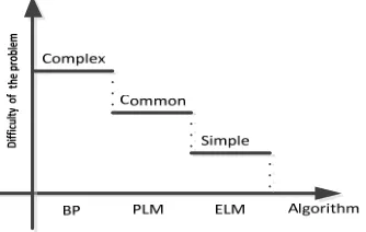
We believe that different learning schemes should be used for solving problems with different difficulty levels: 1) ELM for the easy problems, 2) BP for the complex problems and 3) PLM for the common problems. The relationship between the difficulty of learning and the algorithm is shown in Fig. 1.
Figure 1. The relationship between the difficulty of learning and algorithm.
The differences among the three learning algorithms lie in the number of adjustment parameters, which is shown in Fig. 2. The more complex algorithms, the more parameters in different layers need to be adjusted. As the complexity of PLM is in the middle of ELM and BP, the adjustable parameters of PLM should be neither too large nor too small.
Figure 2. The parameters to be adjusted of the three algorithms.
BP Algorithm and Extreme Learning Machine. For N arbitrary distinct samples )
, X
( i Ti , where
[
]
m T im i ii x x x R
x ∈
= , , ,...,
Xi 1 2 3 , Yi∈R. The model’s predictive output is
represented by:
=⋅⋅
⋅
=
+
⋅
=
Li
i j
i
g
X
b
j
N
O
1j
β
(
ω
i)
,
1
,
,
(1)where L indicates the number of hidden neuron, ωi is the input weights of the hidden node, b is the bias of the hidden neuron, i βi represents the output weights, and
) (
g x is the activation function of the hidden neuron. The cost function is expressed as:
2
1 j j
)
(
=−
=
NO
Y
jE
(2)
The hidden layer output matrix of the neural network is denoted by H, then the Eq. 2 can be simplified as: E=||Hβ−Y||.
[image:2.612.217.421.357.438.2]adjustable parameter space of the network as (W,b,β). The input weights of the network is defined as W [ ]T
L 2 1,ω ,...,ω ω
= , and the bias of hidden neurons is confined
as T
L
b b
b, ,..., ]
[ 1 2 =
b . Therefore, the objective function can be expressed as follows:
||
-)
,
(
||
min
||
-ˆ
)
ˆ
,
ˆ
(
||
,
H
W
Y
Y
W
H
W
b
β
β
b
β b,=
(3)The gradient-based learning algorithms are generally used to search the minimum of Eq. 3.
There are several issues on BP learning algorithms such as easily result in over fitting, cannot ensure that a global minimum will come out and sensitive to the setting of the learning rate.
In order to overcome the shortcomings of error back-propagation learning algorithm, Huang proposed a new learning algorithm for the single-layer FNN, which is called ELM, and proved that the existence of the output weights βˆ makes the cost function
ε < − ||
||Hβ Y . ELM makes the cost function E as small as possible:
||
-||
min
||
-ˆ
||
H
β
Y
H
β
Y
β
=
(4)
The calculation formula of the optimal output weights:
Y
H
+ˆ
=
β
(5)where H+ is the generalized inverse of matrix H [7]. In the process of parameter
adjustment, ELM don't have to adjust the input weights and the biases of the neural network, which could generate one of the least squares solutions of a general linear system Hβ=Y.
Heuristic Adjustment for Partial Learning Machine. Reviewing those disadvantages of BP and ELM, a heuristic partial learning machine (PLM) is proposed. PLM is required to adjust output weights and hidden layer biases, the objective function is: || -) ( || min || -ˆ ) ˆ (
|| H b β Y H b β Y
β b, =
(6)
The output weights are calculated by the method of least square: βˆ=H+T.
This paper puts forward a heuristic method to adjust the bias of the hidden neurons. The bias of the hidden neuron is adjusted in turn, and the following is the heuristic adjustment of the one hidden neuron.
The heuristic adjustment is divided into two stages:
The first stage: Calculating the initial size of the hidden layer bias, which is referred to the learning point. The bias of the hidden neuron needs to be adjusted significantly. Taking a part of the learning point in the setB, B=
{
0.1k|k=1,...,9}
, the Objectivefunction is:
||
-)
(
||
min
||
-)
ˆ
(
||
H
b
Y
H
b
iY
b i i
β
β
=
(7)Where bi∈B, resulting in the current optimal learning point bˆ from set i B.
The second stage: The search set C is established on the basis of the optimal
{
ˆ ⋅(1−0.01 )| =−15,−14,...,14,15}
= b k k
C i
(8)
At this stage, the bias of the hidden layer neurons should be adjusted within a small range. In this case, the adjustment is made within 15% around the optimum learning point. And the current optimal learning point bˆ*
i will be obtained in the same way as the stage 1, and updating the output weightsβˆ .
Combining the above heuristic adjustment methods, a single-layer feed forward neural network algorithm called partial learning machine (PLM) can be summarized as follows:
PLM algorithm: Given a training setΦ=
{
(Xi,Yi)|Xi∈Rm,Yi∈Rn,i=1,⋅ ⋅⋅,N}
,activation functiong(x), hidden neuron number L, input weights and the hidden neuron biases(ωi,b), and output weightsβ.
Step1: Assign the input weights and the hidden neuron biases (ωi,b) randomly.
Step 2: Calculate the output matrix of the hidden layer nodesH.
Step 3: Calculate the output weightsβˆ .
T H+
= βˆ
Step 4: The first and second stages of the heuristic adjustment are performed on the hidden layer nodes in turn.
Introduction to the Experimental Platform
We estimate the performance from four aspects like training time, testing time, training RMSE and testing RMSE. In order to make a better analysis of the algorithm performance, 100 trials have been conducted for the three algorithms in each dataset. The simulation experiment of three algorithms is carried out in MATLAB 2012a environment, running in a Intel Core i7-4710MQ, 2.5GHZ CPU. There are many different versions of the BP algorithm, a faster BP algorithm called Levenberg-Marquardt algorithm (LMA) is used in our simulations. The activation function used in PLM and ELM is a simple sigmoidal one g(x)=1/(1+exp(−x)). In our experiments, all the inputs are normalized into [0,1].
Performance Evaluation
In this section, the performance of the proposed PLM learning algorithm is compared with the popular algorithms of single hidden layer FNN like LMA and ELM. As for each case, both the training and testing dataset are randomly generated from its whole dataset before each simulation trial. Three classic datasets are used to test the performance of BP, ELM and PLM. For each data set are randomly divided into 70% of the training set and 30% of the testing set.
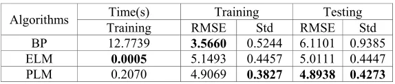
Table 1. Performance comparison for Body Fat dataset (Dataset 1).
Algorithms Time(s) Training Testing
Training RMSE Std RMSE Std
BP 12.7739 3.5660 0.5244 6.1101 0.9385
ELM 0.0005 5.1493 0.4457 5.0111 0.4447
PLM 0.2070 4.9069 0.3827 4.8938 0.4273
It can be seen from Table 1 that the training time value of BP is obviously larger than PLM and ELM. The new PLM runs 61.71 times faster than the BP. The BP trained all the parameters of the entire network, which leads to time-consuming. In the light of the similar testing time of the three algorithms, they have not listed for analysis.
As observed from Table 1 we obtain the following results about training RMSE: BP performs better than PLM and ELM in RMSE evaluation indicators. However, PLM achieves the best performance on indexes Std. Compared with BP, PLM has decreased by 27.02% in index Std. PLM is dropped by 14.14% in index Std when compared with ELM. It shows that PLM is more stable than BP and ELM.
In the testing set PLM are performing better than BP and ELM. BP is the worst performance due to it’s over fitting phenomenon. Compared with BP, PLM has decreased by 19.91% in index RMSE, 54.47% in index Std. Compared with ELM, the index RMSE of PLM has decreased by 2.34% and 3.91% in index Std. The results show that the generalization ability and stability of PLM is better than that of BP and ELM.
Chemical Dataset. There are 498 samples in this dataset [9]. The sample consists 8 inputs, 1 output. The number of hidden nodes of the three algorithms in this case is 20. On the Chemical dataset, the performance of the three different algorithms is shown in Table 2.
Table 2. Performance comparison for Chemical dataset (Dataset 2).
Algorithms Time(s) Training Testing
Training RMSE Std RMSE Std
BP 16.2575 0.8613 0.1558 2.6346 0.4761
ELM 0.0012 2.1126 0.0832 2.4559 0.1490
PLM 1.6179 1.9625 0.0787 2.4176 0.1764
BP has the longest training time and the average training time is about 10.05 times than that of PLM. Similar to the dataset 1, the training time of the BP algorithm on this dataset is still the longest.
As for training set. Seen from Table 2, we got the following results. Since all parameters are trained, the training time of BP is the longest. BP has the best performance in indexes RMSE. However, the training stability of BP is poor. PLM has decreased by 49.49% in index Std when compared with BP. Compared with ELM, PLM decreased by 7.10% and 5.41% separately in the index of RMSE and Std. It illustrates that PLM have a greater improvement in training accuracy than ELM, and the stability of the algorithm is better than BP.
As observed from testing set, it is clear that the index RMSE of PLM is the smallest and the generalization ability of PLM is the strongest while that of BP is the weakest. Compared with the BP, the PLM has decreased by 8.24% in index RMSE and 62.95% in index Std. Compared to ELM, the index RMSE is reduced by about 1.56%.
three different algorithms is shown in Table 3. BP has the longest training time and the average training time is 11.84 times than that of the PLM.
Table 3. Performance comparison for Boston housing dataset (Dataset 3).
Algorithms Training Time(s) RMSE Training Std RMSE Testing Std
BP 19.3492 0.5027 0.7377 12.832 9.3518
ELM 0.0017 4.7425 0.2340 4.6449 0.3086
PLM 1.6343 4.3988 0.2435 4.4007 0.3057
Table 3 indicates that the stability of PLM is much better than that of BP, and the training accuracy of PLM is greater than that of ELM. Compared with the BP, PLM has decreases by 66.99% in index Std. Compared with ELM; PLM has decreased by 7.25% in index RMSE and 6.14% in index Std respectively. There occurs a serious over-fitting phenomenon on BP algorithm in our simulations, as shown in Table 3.
As for the testing set, the two indexes (RMSE, Std) values are the smallest in PLM. PLM is 65.71% in index RMSE and 96.73% in index Std smaller than that of BP. The index Std of PLM is the smallest, which proves that PLM is more stable than ELM and BP.
Conclusions
According to the above experimental results, we can draw conclusions as follows: BP: slow learning speed, extremely high training accuracy, easily fall into local minima and poor generalization ability; ELM: especially fast learning speed, high training accuracy, large random fluctuation, ordinary generalization ability; PLM: fast learning speed, high training accuracy, strong generalization ability, tiny fluctuations and firm stability.
The adjustment in PLM is a kind of heuristic adjustment method. Other fast optimization methods such as gradient descent, conjugate gradient descent, particle swarm algorithm can be used to achieve the purpose of partial learning.
Acknowledgement
This work has been partially funded by the Start Funding for Minjiang Chair Professor under grand 510146. The Project of Fujian Province Key Laboratory of Network Computing and Intelligent Information Processing under Grant No. 2009J1007. Application Demo of Industry Network Control System in Rail Transportation, Information Technology Application "Doubling Plan" by Ministry of Industry, China.
References
[1] F. Rosenblatt. Principles of Neurodynamics: Perceptrons and the Theory of Brain MechanismsSpartan Books, Washington, D.C(1961).
[2] D.E. Rumelhart, G.E.Hinton, R.J. Williams. Nature 323(1986)533-536. [3] M.F. Moller. Neural Networks 6(4) (1993)525-533.
[4] N. Yamashita, M. Fukushima. Computing 15(Suppl.) (2001)237-249.
[6] H.-J. Rong, G.-B. Huang, N. Sundararajan, P. Saratchandran. IEEE Transactions on Systems, Man, and Cybernetics—Part B: Cybernetics 39(4) (2009)1067-1072. [7] D.W. Marquardt. SIAM J. Appl. Math 11(1963)431-441.
[8] K.W. Nelson et al. Medicine and Science in Sports and Exercise 17(2) (1985):189-189.
[9] Neural Network Toolbox User’s Guide.Mathworks Inc, 2012a.