Semi Quantitative Modeling for EMD

2017 3rd International Conference on Electronic Information Technology and Intellectualization (ICEITI 2017) ISBN: 978-1-60595-512-4

Semi-Quantitative Modeling for EMD

Chenxi Shao, Zhizhi Zhu, Qiyu Shao, Xingfu Wang, Fuyou Miao,

Weihua Wang and Ying Zhang

ABSTRACT

In this paper, fully considering that the end effect is an uncertain problem in essence, we proposed a semi-quantitative modeling method, called SQME, to mitigate the effect. By SQME, the qualitative behaviors and the extreme points at both ends are predicted well in the time domain, and the data extension is more reasonable. The feasibility of SQME is illustrated in theory. The simulation and experiment results show that SQME can mitigate the end effect of EMD effectively, and the standard error between the extended series and the actual series is controlled within 1%.

INTRODUCTION

Since the EMD[1] method was first introduced, the domestic and overseas scholars have raised a study upsurge of the EMD basic theory and obtained many results. The EMD method has been widely used in many fields [2]-[4]. Many outstanding problems related to the method, however, still need to be resolved. In the process of EMD, there will lead to disperse at the end, and this disperse would progressively empoison the whole data and cause distortion to the results seriously when both ends of the data are not the local extreme points. This phenomenon is referred as “end effect” [5].

_________________________

Chenxi Shao (Corresponding author, [email protected]); Zhizhi Zhu; Xingfu Wang, Fuyou Miao, Weihua Wang. Department of Computer Science and Technology, University of Science and Technology of China. Hefei, China, 230027.

Qiyu Shao, Department of Computer Science, Dayananda Sagar Institutions, Bangluer University. Bangluer, India, [email protected].

N.E. Huang and his research team tried to forecast the original signal by adding several characteristic waves at both ends [1]. However, they failed to mention how to establish suitable characteristic waves. Recently, many data extension methods have been put forward to restrain the end effect of EMD, such as the time series forecasting method based on the mirror extending method[6], the neural networks method [7], the waveform matching method [8], and so on.

In this paper, fully considering that the end effect has uncertainty and belongs to the qualitative problems with incomplete knowledge, we propose a semi-quantitative modeling method, called SQME, to mitigate the effect, which is based on the method combining qualitative analysis and quantitative analysis according to the essential characteristic of the end effect. This SQME method fully takes into account the interior features and the varying characteristics of the original signal. By virtue of SQME, the data extension is more reasonable. The paper will demonstrate that SQME can deal with the end effect of EMD effectively from the theoretical and experimental aspects. And the experimental results show that the SQME method can control the standard error between the extended series and the actual series within 1%.

THE EMD METHOD AND END EFFECT

The EMD Method

The EMD method separates a complex signal into several Intrinsic Mode Functions (IMFs) [5].

The following is the definition of an IMF:

In the whole dataset, the number of extrema and the number of zero-crossings must either equal or differ at most by one;

At any point, the mean value of the envelope defined by the local maxima and the envelope defined by the local minima is zero.

With the above definition of an IMF, we can then decompose any time series as follows.

-- Let x t( ) be a time series, identify all the local extrema of x t( );

-- Connect all the local maxima to produce the upper envelope, and repeat the procedure for the local minima to produce the lower envelope. And then, calculating

the mean value of the upper and lower envelopes m1_;

-- The difference between the data x t( ) and m1 _{is the first component} h1_:

h1x t( )m1 (1)

-- In principle, h1 _{should be an IMF. In reality, however, usually} h1 _{does not}

times as is required to reduce the extracted signal to an IMF. In the next step, h1 _is

treated as the new data, repeat the previous process up to K times until h1k _becomes

an IMF c1_;

-- Overall, c1 _{should contain the finest scale or the shortest period component of}

the signal. Then c1 _{can be separated from the rest of the data by}

r1x t( )c1 ₍₂₎

-- Since the residue r1 _{still contains longer period variations in the data, it is}

treated as the new data and subject to the same sifting process as described above.

This procedure can be repeated with all the subsequent ri_{, and the result is}

r1x t( )c1；r2 r1 c2； _···rn rn1cn ₍₃₎

The sifting process can be stopped finally by any of the following predetermined

criteria: either when the component cn _{or the residue} rn _{becomes so small that it is}

less than the predetermined value of substantial consequence, or when the residue rn

becomes a monotonic function from which no more IMFs can be extracted. By summing up, we finally obtain:

1

( )

n

i n i

x t c r

 



(4)

End Effect

It is necessary to extend two maxima and two minima at both ends respectively in the every iteration of EMD. And the new extreme points are used to construct the spline curves as interpolation points too. Both ends, however, may or may not be the extreme points, so we must carry on the reasonable predict. Because the quantitative expressions are difficult to build at both ends and such forecasts are, of course, highly uncertain which in essence belong to uncertain problems, the qualitative analysis should be introduced to deal with the problem.

THE SQME METHOD

The SQME method introduced in this paper is based on the QSIM algorithm proposed by B.J. Kuipers [9]. In actual conditions, the data flow we get can be considered as a combination of the real signal and certain noises. The qualitative process is to deal with the data flow to get its qualitative states considering the effect of the noises. The final results are several monotonically increasing or decreasing intervals of the given data flow, and the qualitative states (increase, steady, decrease)

of each interval represented by the corresponding symbols （ ，， ）   .

In order to qualitatively process a time and frequency signal, we first divide the amplitudes of the whole waveform into several phases and define the Quantity Space and Phase Space for the system according to the specific amplitude distribution, so that a point in phase space characterizes the state of the system. Then we use the Qualitative Kernel Function to process the actual data flow for getting the qualitative variation states from the observed data flow of the system. The main steps are as follows.

1） normalize the original signal

Let x t( ) x0,...,xf

be a time series, a normalization of the values of x t( ) is

performed. The different amplitudes are converted into the interval [0,1]. Let

0

( ) ,..., f

x t  x x

be the normalized temporal series obtained from x t( ) . The

formula [12] is given as follows:

0

0 0

min( ,..., )

max( ,..., ) min( ,..., )

i f

i

f f

x x x x

x x x x

 

 (5)

Where min and max are operations that return the maximum and the minimum value of a numerical sequence respectively.

2） Compute the difference seriesx_D

Let xD  d0,...,df1 _{be the difference series obtained from ( )}x t _{as follows:}

di xi1xi ₍₆₎

The amplitudes are converted into the interval [-1,1].

3） Define Quantity Space

A quantity space is a qualitative abstraction of the real signal, divided by landmark values into points and intervals. We define quantity spaces and assign the

qualitative labels to represent phase spaces according to the difference series xD_.

The labeling process is defined based on the parameters  and i₍i_{), which}

by the experts according to the knowledge about the system, and influenced by the sampling frequency of the original signal of the system. In this paper, we define them mainly based on the experimental observation. Usually the values of the

parameters  and i _{will make all states of the phase spaces exist, and the results of}

the similar states keep steady when  changes in a certain range at the value.

Generally, this step for the semi-quantitative modeling method is inspired by the way of qualitative modeling and simulation [10] [13][14].

4） Identify The Qualitative Variation States

We use the qualitative processing method based on the normalized and differential fitting principle to deal with the original data flow.

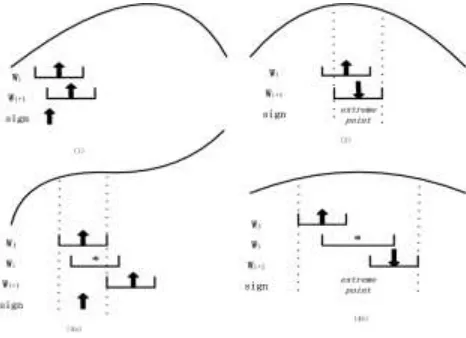
The Qualitative Kernel Function k W( i) _{is the core of the qualitative}

processing method. This function deals with window Wi _{which starts from the i-th}

data point, and we denote Ti _{as the length of the window. Function} k W( i) returns

the following results:

 Wi consists of a monotonically increasing segment;

 Wi _{consists of a monotonically decreasing segment;}

 Wi_{has no monotonicity.}

We get the complete qualitative trends of the whole data flow, and transform them into Quantity Space, and use the symbols of Quantity Space to replace every trend for getting the qualitative behaviors and states of the original signal system. Then the next quantitative states at both ends can be predicted from the successors of their equivalent states in the set of internal qualitative states. Two qualitative

states are equivalent if and only if both parameters share the same nodal value in their corresponding path, and the directions of their variation are also the same. At last, we can extend the data flow at both ends by using model calculation.

MODEL CALCULATION

Model Calculation

We take full account of the variation characters of the amplitude values of signal, and build the model according to the above SQME method.

First, apply the normalization method and the difference method to the original

signal for getting the difference series xD  d0,...,df1

. The amplitudes are converted into the interval [-1,1]. Then we divide out quantity spaces according to

the difference series xD_{. The parameters}  _and i₍i_{) can be flexibly adjusted}

according to xD_.

Next, use the Qualitative Kernel Function to process the original data flow, and

simply define the length of the window Ti _{as a data point interval to get the}

qualitative variation trends. And then transform the trends into Quantity Space, and use the symbols of Quantity Space to produce Phase Space and the qualitative

character sequence Sx  c1,...,cf1 _{, where every} ci _{represents the evolution of the}

curve between the two adjacent time points in the original signal. This translation abstracts from the real values and focus our attention on the shape of the curve. Every sequence of symbols describes a complete family of curves with a similar evolution.

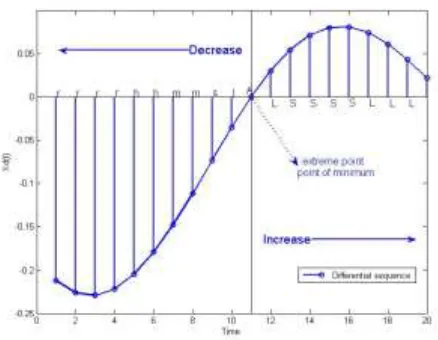
Fig.2 shows the qualitative character sequence of an actual signal after the normalization processing, difference processing, and labeling processing.

At last, find the equivalent states or the most similar behavioral states to the states at both ends in the set of internal qualitative states. Because of only one

difference data point in the window Wi _{, we can use the characters matching}

algorithm to search the equivalent states or the most similar behavioral states in the Quantity Space.

Error Analysis

The paper uses the standard error to measure the forecasting effect of SQME.

Let the predicted results of the extended series at both ends be x x1, 2,...,xn _and

the corresponding true values be y y1, 2,...,yn_{, then the standard error}  _{of the}

extended series at both ends is[11]:

2 2 2 2

1 1 2 2

(x y) (x y ) (x_n y_n) (x_i y_i)

n n

           (12)

In this paper, we use the arithmetic mean values (they are nearest the true values), on the basis of many repeated experiments supported by modifying the

parameter  in certain ranges, instead of the true values when making the error

analysis for real-world signals.

Standard error is not an actual error and an error range, but the reliability of estimate of the predicted values. The smaller the standard error is, the larger the degree of reliability. Conversely, the forecast is less reliable.

SIMULATION EXPERIMENTS

A Typical Nonlinear Signal

Take the following signal for example, which is:

2 2 2

( ) cos( ) 0.6 cos( ) 0.5sin( )

50 25 200

x t  t  t   t t





(13)

The signal is plotted in Fig.3. The solid line represents the original signal. The green dash and red dash line represents the upper and lower envelops of the signal respectively. It is shown that there are only three maxima and four minima in the original signal and the resulting envelops fail to include all of the data. Especially the upper envelope appears to be hugely distorted on the two ends of the data. At the same time, the original signal is so short that end effect would empoison the whole data and the decomposition results would be meaningless. Therefore, it is essential to restrain the end effects when EMD method is applied to the signals.

First, normalize the original signal and designate the normalization series as '

( )

x t _.

Second, compute the difference series xD _from

'

( )

x t _{. The parameteriis set to 2.}

The parameter  should be adjusted constantly from 3 (i_{) until all the states of}

Phase Space exist and the results of the similar states keep steady. In this

experiment, the range of parameter  is from 15 to 18. Then, define Quantity Space

and apply the Qualitative Kernel Function to the signal to produce the qualitative

character sequence Sx_{, which represent the states of Phase Space, consisted of the}

Symbols of the xD_.

The results in this experiment show that neither of both end points is the local extreme points by judging the general trends of them, so we need to predict the positions of the extreme points first. And then calculate the values of the extended extreme points depending on their positions.

The real components of the original signal and the components of the extended time series are shown in Fig.4.

As Fig.4 shows, the proposed new method can effectively suppress the undesirable end effect unavoidable in EMD. The IMFs of the extended time series are correspondent with the true IMFs of the practical original signal.

Use the standard error to measure the forecasting effect, and conduct ten

independent experiments for each value of parameter  between 15 and 18. The

best standard error is 0.3%, and every time the standard error is no more than 1%. The experimental results demonstrate the accuracy and superiority of SQME when dealing with End effect of the short time series.

A Classic Nonlinear System

The Rossler equation is one of the classic nonlinear equations with the form, Figure 4. Real IMFs of the Original

Time Series and IMFs of the Extended Time Series. The solid line represents Real IMFs of the Original Time Series. The dash line represents the IMFs of the extended time series.

( )

dX dt  Y Z ₍₁₄₎

dY dt X Y ₍₁₅₎

( )

dZ dt  Z X ₍₁₆₎

0.2

 ₍₁₇₎

0.2

  (18)

3.5

  (19)



 



(20)

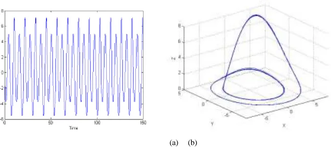
The values of the parameters



values in [15] for comparison. Fig. 5 presents the phase diagram and the time series of the x-component. This system contains exactly two time scales, and the wave form of the x-component is regular with an exact period of twice the high-frequency oscillation.

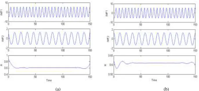
Applying the EMD method to the x-component without using any extending method, we have only three IMF components as shown in Fig. 6(a). The IMFs, however, are distorted on the two ends of the data, especially for the second one. Then, using the proposed semi-quantitative method for the end effect of EMD, we have better results of decomposing as shown in Fig. 6(b): a seemingly uniform high-frequency component; an intermediate frequency component; and a low-intensity and low-frequency component with non-zero mean. The decomposing results agree well with the results in [15].

(a) (b)

In this study, we use the arithmetic mean values of dozens of repeated

experiments supported by modifying the parameter  in certain ranges, instead of

true values to compute the standard error, and the standard error is about 0.8%.

CONCLUSIONS

Generally speaking, in previous works there was no method effective and applicative to any non-linear and non-stationary time series for the end effect of EMD. Existing methods either have poor adaptability to some time series or would take a long time. But the SQME method can be applied to every case. On one hand, the method has robust characteristics and it is self-adaptive and can run smoothly at all times, which is already explained in the theoretic analysis of the method. On the other hand, the most time-consuming operation of SQME, string match, can be fully finished in a short time by adopting existing efficient algorithms such as KMP and so on.

In a word, SQME, the proposed simple and feasible method, can be applied in practical production for the end effect of EMD.

ACKNOWLEDGEMENT

This work is supported by the Natural Science Foundation of China (NSFC) under Grant No. (61472381, 61472382, 61572454 and 61174144), NOE-Microsoft Key Laboratory of Multimedia Computing and Communication Foundation, Anhui Province Key Laboratory of Software in Computing and Communication.

REFERENCES

1. N.E. Huang, Z. Shen, S.R. Long, M.L. Wu, H.H. Shih, Z. Quanan, N.C. Yen, C.C. Tung, and H.H. Liu. 1998. "The empirical mode decomposition and the Hilbert spectrum for nonlinear and non-stationary time series analysis". Proc. Roy. Soc. Lond. A, Mar.

(a) (b)

2. N.E. Huang, M.L. Wu, S.R. Long, S.P. Shen, W. Qu, P. Gloersen, and K. Fan. 2003. "A confidence limit for the Empirical Mode Decomposition and Hilbert Spectral Analysis". Proc. Roy. Soc. Lond. A, April.

3. N.E. Huang, Z. Wu, S.R. Long, K.C. Arnold, K.Blank, and T.W. Liu. 2009. "On instantaneous frequency". Advance in Adaptive Data Analysis. 1(2):177-229.

4. N.E. Huang and Z. Wu. 2008. "A review on Hilbert-Huang transform: method and its applications to geophysical studies". Rev. Geophys., 46:108-118.

5. N.E. Huang and S.P. Shen. 2005. "Hilbert-Huang Transform and Its Applications". 1st ed. New York: World Scientific, Jun.

6. J.P. Zhao and D.J. Huang. 2001. "Mirror extending and circular spline function for empirical mode decomposition method". Journal of Zhejiang University(Science), 2(3):247-252.

7. Y.J. Deng and W. Wang. 2001. "Dealing with the End Effect of EMD and Hilbert-Huang Transform". Chin. Sci. Bull., 46:257-263.

8. C.X. Shao and J. Wang. 2007."A Self-Adaptive Method Dealing with the End Issue of EMD".Acta Electronica Sinica, 35:1944- 1948.

9. B.J. Kuipers. 1986. "Qualitative simulation". Artif. Intell., 29:289-338.

10. J.K. George. 1991. "Aspects of Uncertainty in Qualitative Systems Modeling". Qualitative Simulation Modeling and Analysis, SpringerVerlag, New York, Inc.

11. Wikipedia. 2017. "The free encyclopedia. Standard error (statistics)" [Online]. Available: http://en.wikipedia.org/wiki/Standard_error_(statistics).

12. S. Qiang and Roy Leitch. 1993. "Fuzzy Qualitative Simulation". IEEE Trans. on Systems, Man, and Cybernetic, 23(4):301-313.

13. B.J. Kuipers. 1994. "Qualitative reasoning: modeling and simulation with incomplete". Massachusetts Institute of Technology, Press, 378.

14. B.J. Kuipers and D. Berleant. 1998. "Using incomplete quantitative knowledge in qualitative reasoning". Proc. Nat. Conf. On Artificial Intelligence, Morgan Kaufman, Los Altos, California, July.