3D Panoramic Imaging for Virtual Environment Construction

Gledhill, Duke

3D Panoramic Imaging for Virtual Environment Construction

Original Citation

Gledhill, Duke (2009) 3D Panoramic Imaging for Virtual Environment Construction. Doctoral  thesis, University of Huddersfield. 

This version is available at http://eprints.hud.ac.uk/id/eprint/6981/

The University Repository is a digital collection of the research output of the University, available on Open Access. Copyright and Moral Rights for the items on this site are retained by the individual author and/or other copyright owners. Users may access full items free of charge; copies of full text items generally can be reproduced, displayed or performed and given to third parties in any format or medium for personal research or study, educational or not­for­profit purposes without prior permission or charge, provided:

• The authors, title and full bibliographic details is credited in any copy; • A hyperlink and/or URL is included for the original metadata page; and • The content is not changed in any way.

For more information, including our policy and submission procedure, please contact the Repository Team at: [email protected].

Construction

A Thesis Submitted to the University of Huddersfield in Partial Fulfilment of the Requirements for the Degree of Doctor of Philosophy

by

Duke Gledhill BSc (Hons) School of Computing and Engineering

The University of Huddersfield

In Collaboration with Rotography Ltd

Sponsored by the EPSRC

The project is concerned with the development of algorithms for the creation of photo-realistic 3D virtual environments, overcoming problems in mosaicing, colour and lighting changes, correspondence search speed and correspondence errors due to lack of surface texture.

A number of related new algorithms have been investigated for image stitching, content based colour correction and efficient 3D surface reconstruction. All of the investigations were undertaken by using multiple views from normal digital cameras, web cameras and a ”one-shot” panoramic system. In the process of 3D reconstruction a new interest points based mosaicing method, a new interest points based colour correction method, a new hybrid feature and area based correspondence constraint and a new structured light based 3D reconstruction method have been investigated.

The major contributions and results can be summarised as follows:

• A new interest point based image stitching method has been proposed and in-vestigated. The robustness of interest points has been tested and evaluated. Interest points have been proved robust to changes in lighting, viewpoint, rota-tion and scale.

• A new interest point based method for colour correction has been proposed and investigated. The results of linear and linear plus affine colour transforms have proved more accurate than traditional diagonal transforms in accurately matching colours in panoramic images.

• A new structured light based method for correspondence point based 3D recon-struction has been proposed and investigated. The method has been proved to

area based correspondence search constraint.

• Based on the investigation, a software framework has been developed for image based 3D virtual environment construction. The GUI includes abilities for im-porting images, colour correction, mosaicing, 3D surface reconstruction, texture recovery and visualisation.

• 11 research papers have been published.

1. M. Bingham, D. Taylor, D. Gledhill, Z. Xu, ”Integration of Real and Virtual Light Sources in Augmented Reality Worlds”, 14th International Conference on Automation and Computing. Pacilantic International, ISBN 978-0955529320, pp 75-80. Brunel University, UK, September 2008.

2. G. Y. Tian, R. Lu, D. Gledhill,”Surface Measurement Using Active Vision and Light Scattering”, Optics and Lasers in Engineering, Vol. 45, Issue 1. Elsevier Science, ISSN 01438166, pp 131-139. 2007.

3. G. Y. Tian, D. Gledhill ”Visualisation Based Feedback Control for Multiple Sensor Fusion”, 10th International Conference on Information Visualization (IV’06). IEEE Computer Society, ISSN 1550-6037, pp 553-556. London, UK, July 2006.

4. R. Lu, G. Y. Tian, D. Gledhill, S. Ward,”Grinding Surface Roughness Measure-ment Based on the Co-occurance Matrix of Speckle Pattern Texture”, Applied Optics, Vol. 45, Issue 35. Optical Society of America, pp 8839-8847. December 2006.

5. D. Gledhill, G. Y. Tian, D. Taylor, D. Clarke, ”Panoramic Imaging Based e-laboratory Construction”, The Book of Advances in e-Engineering and Digital Enterprise Technology (e-ENGDET). Wiley, ISBN 978-1860584671, pp 589-600. August 2004.

6. G. Y. Tian, D. Gledhill,”Structured Light Based Stereo Vision for Coordination of Multiple Robots”, 1st International Conference on Informations in Control,

Setubal, Portugal, August 2004.

7. C. Mitchell , G. Y. Tian, D. Gledhill, D. Taylor, ”Web-based Interactive 3D Visualisation for Business and Building Management”, Proceedings of the 8th IASTED International Conference on Internet and Multimedia Systems and Applications (IMSA). ACTA Press, ISBN 0-88986-420-9. Kauai, Hawaii, USA, August 2004.

8. D. Gledhill, G. Y. Tian, D. Taylor, D. Clarke, ”3D Reconstruction of a Re-gion of Interest Using Structured Light and Stereo Panoramic Images”, 8th In-ternational Conference on Information Visualisation (IV’04). IEEE Computer Society, ISBN 0-7695-2177-0, pp 1007-1012. London, UK, July 2004.

9. D. Gledhill, G. Y. Tian, D. Taylor, D. Clarke,”Panoramic Imaging - A Review”, Computers and Graphics 27(3), ISSN 0097-8493, pp 435-445. 2003.

10. G. Y. Tian, D. Gledhill, D. Taylor,”Comprehensive Interest Point Based Imag-ing Mosaic”, Pattern Recognition Letters 24(9-10). ISSN 0167-8655, pp 1171-1179. 2003.

11. G. Y. Tian, D. Gledhill, D. Taylor, D. Clarke,”Colour Correction for Panoramic Imaging”, 6th International Conference on Information Visualisation (IV’02). IEEE Computer Society, ISBN 0-7695-1656-4, pp 483-488. London, UK, July 2002.

2.1 A complete panorama . . . 6

2.2 Kaidan Kiwi990 with Nikon Coolpix 990 camera . . . 8

2.3 Diagram showing panoramic capture process for single camera where P_n = Photo, P_c = combined panorama and O = optical centre of the camera. . . 9

2.4 A 360◦ by 120◦ panoramic image . . . 10

2.5 iMove SVS-2000 Camera System . . . 11

2.6 Two 180◦ hemispheres that can be used to create an omni directional image . . . 12

2.7 BeHere Video System uses a mirror to capture the environment . . . 13

2.8 The first true stereo camera with two lenses, built in 1849 . . . 14

2.9 A modern stereo camera setup . . . 14

2.10 Altering the rotation point and using different parts of the images to create a stereo panorama . . . 15

2.11 Original image, and position information provided by edge detector . 20 2.12 Left original image before the mosaicing . . . 30

2.13 Right original images before the mosaicing . . . 30

2.14 Two images stitched together (without blending) . . . 31

2.15 Two images stitched together (with blending) . . . 31

2.16 3D surface reconstruction . . . 32

2.17 Stereo images and related disparity map . . . 35

2.18 Epipolar geometry and epipolar plane . . . 36

2.19 Triangulation to find a point in 3D from 2 2D images . . . 38

4.1 Stereovision system and panoramic imaging for 3D virtual environment 53 4.2 Showing the process of 3D panoramic imaging Where FOE is the Focus

of Expansion and FOC is the Focus of Contraction, both parts of a panorama where either too much (FOE) or too little (FOC) depth is

perceived. . . 54

4.3 The one-shot system . . . 56

4.4 The multi-shot system, showing 4 of the 26 positions used . . . 57

4.5 Stereo system using web cameras for stereo correspondence algorithm testing . . . 57

4.6 Diagram showing multi-shot system camera orientations. . . 58

4.7 Screenshot of software framework. . . 59

4.8 A diagram of the software framework . . . 60

4.9 Crops from consecutive images from a panorama sequence showing colour changes due to capture devices settings changes . . . 62

5.1 Step 1 of the new approach of colour correction . . . 64

5.2 Step 2 of new approach of colour correction . . . 65

5.3 Linear transform matrix estimation and colour correction before image stitching and panorama . . . 66

5.4 Histogram before and after equalisation . . . 68

5.5 Overlapping area of the stitching images . . . 71

5.6 Colour correction based on M orM −1 . . . 71

5.7 A selection of images used in the experimental tests for the colour correction algorithms . . . 89 5.8 Comparison of the speed for the colour correction pre-processing methods 90 5.9 Comparison of accuracy for the colour correction processing methods 91

variations . . . 93

5.12 Comparison of the standard deviation in processing time for each pre-processing method . . . 94

5.13 Comparison of the minimum, mean and maximum processing times for each pre-processing method . . . 95

5.14 Different colour correction for panoramic imaging . . . 97

6.1 Image mosaic processing block-diagram . . . 99

6.2 Interest points across illumination and rotation . . . 101

6.3 Rotation-invariant LBP . . . 103

6.4 Two stitching images and their corresponding points . . . 104

6.5 Stitched image without colour correction . . . 105

6.6 The stitched images with colour correction . . . 108

6.7 A selection of images used in the experimental tests for the feature matching algorithms . . . 110

6.8 A comparison of the average accuracy (%) of the feature matching algorithms . . . 115

6.9 A comparison of the average speed (seconds) of the feature matching algorithms . . . 115

6.10 A comparison of the minimum accuracy (%) of the feature matching algorithms . . . 116

6.11 A comparison of the minimum speed (seconds) of the feature matching algorithms . . . 116

6.12 A comparison of the maximum accuracy (%) of the feature matching algorithms . . . 117

6.14 A comparison of the standard deviation of accuracy (%) of the feature matching algorithms . . . 118 6.15 A comparison of the standard deviation of speed (seconds) of the

fea-ture matching algorithms . . . 118

7.1 An example of the structured light pattern to be projected onto low texture surface areas . . . 121 7.2 Showing the structured light pattern in an image (left) and after it has

been removed (right) . . . 122 7.3 Showing the results of 3D depth calculations when no structured light

pattern used . . . 123 7.4 Showing the results of 3D depth calculations when structured light

pattern used . . . 124 7.5 Structured light pattern projection results showing fewer errors in the

depth map where the structured light is projected (inside the red line) 125 7.6 Interest points and their correspondence . . . 125 7.7 Computing expense and search area . . . 126 7.8 Corresponding areas for constrained area based searching (Left image

and right image) . . . 127 7.9 Process using interest points to increase the speed of processing the 2D

data . . . 128 7.10 The stereo images and their disparity map, using area based method

of correspondence searching . . . 128 7.11 Brick data showing Interest points and correspondence matches, and

disparity map . . . 129

8.1 Embedded 3D virtual environment for Web-based interactive applications131

5.1 Average (mean) values for all colour correction image tests . . . 73

5.2 Minimum values for all colour correction image tests . . . 74

5.3 Maximum values for all colour correction image tests . . . 75

5.4 Standard Deviation for all colour correction image tests . . . 76

5.5 Average (mean) values across the brightness variation colour correction test images . . . 77

5.6 Minimum values across the brightness variation colour correction test images . . . 78

5.7 Maximum values across the brightness variation colour correction test images . . . 79

5.8 Standard Deviation of values across the brightness variation colour correction test images . . . 80

5.9 Average (mean) values across the white balance variation colour cor-rection test images . . . 81

5.10 Minimum values across the white balance variation colour correction test images . . . 82

5.11 Maximum values across the white balance variation colour correction test images . . . 83

5.12 Standard Deviation of values across the white balance variation colour correction test images . . . 84

5.13 Average (mean) values across the white balance and brightness varia-tion colour correcvaria-tion test images . . . 85

5.15 Maximum values across the white balance and brightness variation colour correction test images . . . 87 5.16 Standard Deviation values across the white balance and brightness

vari-ation colour correction test images . . . 88

6.1 Average Interest Point Correspondence Results (SIFT and Proposed Method) . . . 111 6.2 Minimum values for the interest point correspondence results (SIFT

vs. Proposed Method) . . . 112 6.3 Maximum values for the interest point correspondence results (SIFT

vs. Proposed Method) . . . 113 6.4 Standard deviation values for the interest point correspondence results

(SIFT vs. Proposed Method) . . . 114

I would like to thank the School of Computing and Engineering at the University of Huddersfield for granting me the opportunity to carry out this project. I would also like to thank Rotography Ltd and the EPSRC for co-funding the project.

I would like to express my gratitude to my director of studies, Prof. G. Y. Tian, who has guided and supported me throughout the project. My gratitude also goes to my second supervisor, Prof. D. Taylor for his help and support with the project.

I would also like to thank my parents for supporting and encouraging me through-out my education. They always pushed me to do better, and it doesn’t get much better than a PhD!

The work was very enjoyable and I am very excited about the new Augmented Reality work currently underway. I would also like to keep working on the mosaicing using interest points, the Hugin application currently uses 2 different methods for automatic mosaicing. Developing a 3rd, faster, more accurate method would be very interesting.

Abstract i

List of Publications iii

List of Figures v

List of Tables ix

Acknowledgements xi

Chapter 1: Introduction 1

1.1 Motivation . . . 1

1.2 Aims . . . 3

1.3 Thesis Outline . . . 4

Chapter 2: Literature Survey 5 2.1 Introduction . . . 5

2.2 Image Capture Systems . . . 7

2.2.1 Single and Multi Camera-based Panoramic Systems . . . 7

2.2.2 Omni Directional Imaging Systems . . . 11

2.2.3 Stereo Cameras . . . 13

2.3 Image Processing and Understanding . . . 15

2.3.1 Noise Reduction . . . 16

2.3.2 Radial Lens Distortion Correction . . . 16

2.3.3 Camera Calibration . . . 17

2.5 Image Mosaicing and 3D Reconstruction . . . 26

2.5.1 Mosaicing . . . 27

2.5.2 3D Construction . . . 31

2.5.3 Stereo Panoramas . . . 40

2.5.4 Rendering and 3D visualisation . . . 41

2.6 Discussions . . . 42

2.6.1 Stereo Vision Based Panoramic Capture System . . . 42

2.6.2 Deriving Capturing Conditions and Object Surface Character-istics . . . 43

2.6.3 Image Understanding and 3D Reconstruction . . . 43

2.6.4 Image Based Volumetric Rendering . . . 44

2.6.5 Problems identified . . . 45

Chapter 3: Theory and Project Issues 47 3.1 Project concept and major elements . . . 47

3.2 Key project elements . . . 48

3.2.1 Image capture . . . 49

3.2.2 Pre-processing . . . 49

3.2.3 3D reconstruction . . . 50

3.2.4 Visualisation . . . 50

3.3 Methodology . . . 51

Chapter 4: Panoramic Stereo Imaging 52 4.1 Introduction . . . 52

4.2 System Design . . . 52

4.2.1 Hardware . . . 55

4.5 3D Reconstruction . . . 61

Chapter 5: Colour Correction 63 5.1 Histogram Map Based Colour Correction . . . 63

5.1.1 Histogram Equalisation . . . 66

5.1.2 Histogram Mapping . . . 67

5.1.3 Singular Value Decomposition . . . 69

5.2 Colour Correction for Panoramic Imaging . . . 70

5.3 Experimental Tests . . . 72

5.4 Summary . . . 96

Chapter 6: Image Mosaicing 98 6.1 Introduction . . . 98

6.2 4-step Interest Points Based Image Mosaic . . . 98

6.2.1 Identification of Interest Points . . . 99

6.2.2 Finding corresponding points from stitching images . . . 101

6.2.3 Spatial and Spectral Transform Matrices . . . 103

6.2.4 Image Mosaic with Smoothing . . . 107

6.3 Experimental Tests . . . 108

6.4 Summary . . . 119

Chapter 7: 3D Surface Reconstruction 120 7.1 Introduction . . . 120

7.2 3D Surface Reconstruction Using Structured Light . . . 120

7.3 Interest Point Based 3D Surface Reconstruction . . . 122

7.4 Experimental Tests . . . 126

7.5 Summary . . . 127

8.2 Web-Based Interactive System Using 3D Panoramic Imaging . . . 131 8.3 Video panoramic imaging . . . 132 8.4 Using interest points to integrate the real and virtual world in computer

games . . . 132 8.5 Conclusions . . . 132

Bibliography 135

Chapter 1

INTRODUCTION

1.1 Motivation

do most of the work. Stereo vision is still largely a research area though, as many unresolved problems still exist. A significant problem is the correspondence problem, the most common and difficult for computer vision applications and algorithms. Cor-respondence describes the relationship of a feature or area between different images. Given a point or area in one image, the correspondence problem is that of finding the corresponding point or area in another image.

Recent research work has begun to combine the work of panoramic imaging and stereo imaging to create stereo panoramas. Commercially there is now a product from Autodesk which goes a long way toward this goal, although it is still an online process requiring time consuming user input. With more work in this field, it will ultimately mean the possibility of being able to create entire 3D environments from 2D panoramic images for use in virtual tourism, gaming, film, military, manufacturing and design. It will, in the future, be possible to enter a physical space, capture multiple panoramas at different locations and then create a 3D reconstruction of the scene, with little or no user involvement. Architects, film makers and games programmers could all take advantage of such technology to speed up existing methods of 3D construction.

Applications for a 3D panoramic system include military, tourism, games, film, manufacturing and design. As an example, a “drone” robot could scout a military zone with no risk to humans. The automated drone would capture panoramic data which would be processed in real time to generate a 3D virtual environment for soldiers or commanders to explore before entering the area. Another example might be being able to walk along a virtual beach to see a foreign resort, without leaving the comfort of your home. Games programmers could save time building complex models of famous buildings, just by visiting the building and capturing it in 3D. The success of a system with this capability would depend on accuracy, ease of use, speed and cost.

They are now working toward new technologies such as panoramic video and 3D panoramic imaging. They sponsored this project to further their work in panoramic technologies. They hope to gain useful insights into future technologies to help keep them ahead of the competition. The research is also sponsored by the EPSRC.

The University has a previous research record in the area of signal processing. Gui Yun Tian is a respected researcher in the areas of signal processing and colour correction. Duke Gledhill has a degree in Multimedia Technology from the University of Huddersfield and a personal, and expensive, interest in all technologies related to panoramic imaging.

1.2 Aims

The objective of this project was to develop and improve algorithms used in a 3D panoramic imaging system for fast construction of 3D environments from panoramic images. Experimental work was carried out to determine the most appropriate panoramic capture system for the purpose of 3D reconstruction. Experimental work was also undertaken to determine the most accurate methods of matching the panoramic images, and determining 3D information.

The objectives can be broken down as follows:

• To review current panoramic imaging techniques, from capture through to 3D reconstruction.

• To design a novel 3D panoramic imaging system, comprising capture, processing and visualisation.

• To evaluate the test results and determine new strategies for overcoming any problems.

• To identify the key features of the system and applications for the system.

1.3 Thesis Outline

Chapter 2

LITERATURE SURVEY

2.1 Introduction

As computers and cameras become cheaper, the use of digital images is becoming more prevalent. Panoramic imaging is an important part of this expanding use of digital equipment. The term panorama was first used by the painter Robert Barker to describe his panoramic paintings of Edinburgh. Surrounded by these paintings gave the impression of standing in another environment. Translating that to modern virtual tours, apart from being on a computer screen the feeling of immersion is still present. In its most general sense, a panorama is a single wide-angle image of the environment around the camera. Usually they completely surround the camera on the horizontal plane, and can be either approximately 120◦ in the vertical field of view, or 180◦ to create a complete sphere, but the term is often used to describe any wide angle representation of a scene. An example of a complete 360◦ cylindrical panorama is shown in Fig. 2.1 [10].

Figure 2.1: A complete panorama

camera mounted on a tripod and rotated about its optical centre, using a single omni directional camera, using multiple cameras facing in different directions, or using a stereo panoramic camera from which stereo information can be extracted. There is also another alternative to the stereo panorama for calculating stereo information. Instead of rotating the camera about its optical centre, the camera can be moved and used to capture multiple images of a scene from different viewpoints, from which stereo information can be calculated about the scene. This stereo information can then be used to create a 3D model of the scene, and arbitrary views can be computed. This information could also be used to build 3D models of large areas, for example a city might be reconstructed in this way. The process of the panoramic or stereo system can be simplified to four main stages:

1. Image Capturing System

2. Image Processing

3. Image Stitching or Stereo Processing

4. Rendering and 3D Visualisation

3D panoramic imaging and identify research topics and applications. The rest of the chapter is organised as follows. Section 2.2 introduces image capture systems, section 2.3 discusses image processing and understanding, section 2.4 discusses colour correction, section 2.5 discusses image stitching and structure from stereo and finally 3D visualisation.

2.2 Image Capture Systems

As the technology used in digital cameras becomes cheaper, so do the cameras them-selves. Modern digital cameras have high-resolution sensors, which capture a large amount of data about the scene being photographed. For panoramic imaging n num-ber of images need to be captured, where nis dependent on the camera, lens, and the type of panorama required. Many panoramic image systems have been developed, from cheap off the shelf cameras that take a high number (e.g. >8) of sequential images, to omni directional systems that capture only one image.

The important parts of the imaging systems are:

• Resolution

• Field of view

• Capturing speed

2.2.1 Single and Multi Camera-based Panoramic Systems

Panoramic imaging from multiple images involves either a camera rotated about its optical axis (or nodal point), or using multiple cameras capturing different directions. For a single camera rotated about its optical axis there are several components required

• Lens

• Rotator

• Tripod

The camera and tripod can be relatively standard. The lens choice depends on the field of view required from each image. The lens choice determines field of view and therefore required number of images to capture the full panorama and also ensure enough overlap between images to enable correspondence matching and an accurate mosaic. The rotator is very important, it must enable the camera to rotate about its entrance pupil without flex or movement. An inaccurate rotator will cause parallax errors in the images and make mosaicing difficult or impossible.

From a commercial perspective, all of the above can be acquired easily on the open market. Panoramic imaging systems can start with relatively standard, off the shelf cameras [13, 14], panorama tripod mounts [15, 16] and software [11, 17, 18]. A commercial example might include a Nikon 990 [13] mounted on a Kiwi990 (Fig. 2.2) tripod mount from Kaidan [15], and using Pixaround [17] software to stitch the images. This example system would require several images for an accurate panorama, by altering the lens (e.g. a Nikon 8mm FC-E8), fewer images need capturing.

Figure 2.2: Kaidan Kiwi990 with Nikon Coolpix 990 camera

the panorama is captured by turning the camera on the tripod about the optical centre of the camera (Fig. 2.3) and capturing an image at chosen points. Important considerations include overlap, movement of objects in the scene near the overlap regions and control of camera settings, such as white balance and exposure. Consistent white balance and exposure are important for smooth blending of images.

Figure 2.3: Diagram showing panoramic capture process for single camera where P_n

= Photo, P_c = combined panorama and O = optical centre of the camera.

be kept unchanged. For example changes in white balance and exposure between cap-tures will result in more difficulties for mosaicing and blending images for a seemless panorama.

Advantages of this process are that it can be relatively cheap and easy to use, therefore it has become popular with many photographers. Also the fact that almost any camera can be used on just about any tripod (and rotator) and it makes this type of panorama even more appealing. Some modern cameras even come with panorama assist modes to help in the capture process (e.g. Canon Digital IXUS and Nikon P series cameras).

Figure 2.4: A 360◦ by 120◦ panoramic image

translates into small cameras and with current technology relatively low resolution. As sensor technology improves higher resolution solutions will be possible. Only 4 cameras for 180◦ coverage also requires very wide angle lenses and the issues that exist with them, e.g. distortion and resolving power.

Figure 2.5: iMove SVS-2000 Camera System

2.2.2 Omni Directional Imaging Systems

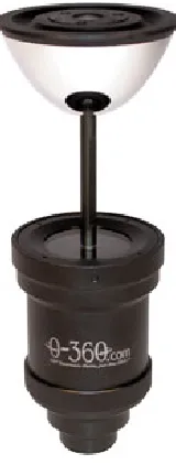
of lens distortion with fisheye lenses which takes processing power to correct, making real time systems a more difficult goal. The low resolution and high lens distortion of the fisheye lens means that accurate distortion free perspective views cannot be cal-culated from images captured with a fisheye lens. Catadioptric imaging systems use a reflecting surface to enhance the field of view. Examples of Catadioptric systems can be found in [21] and commercial examples include the 0-360 one-shot system used in this project [6]. Svoboda et al describe Spherical, Hyperbolic and Parabolic mirror systems and derive information making them useful for stereo panoramic imaging [21]. However, omni directional systems generally suffer from lower resolution, something that will become less of an issue as higher resolution sensors are developed.

Figure 2.6: Two 180◦ hemispheres that can be used to create an omni directional image

Figure 2.7: BeHere Video System uses a mirror to capture the environment

high key and low key images are captured for stitching. This method could not be used for the multi-camera and omnidirectional systems. For omnidirectional sensors bracketing the capture settings of the camera and post processing to create a high dynamic range image can be very effective. As new sensors are developed, higher dynamic range images will be possible.

2.2.3 Stereo Cameras

disparity and accurate correspondence information, computers are able to calculate depth information from a set of stereo images to produce depth maps of the scene.

Figure 2.8: The first true stereo camera with two lenses, built in 1849

Figure 2.9: A modern stereo camera setup

right components are mosaiced to create two panoramas, one for each eye, illustrated in Fig. 2.10.

Figure 2.10: Altering the rotation point and using different parts of the images to create a stereo panorama

2.3 Image Processing and Understanding

The image acquired in the image capture system must now be processed. The pro-cessing is required because the computer does not ’know’ what the images are, and what information they contain, apart from the pixel data. Once the images are pro-cessed they can be used in a panoramic or stereo system. There are many stages to image processing, some which are not used in both stereo and panoramic imaging. For 3D reconstruction and panoramic imaging the image processing can be defined in several stages:

• Noise Reduction

• Radial Lens Distortion Correction

• Feature Detection and Matching

2.3.1 Noise Reduction

Noise is an inevitable part of image processing, particularly when using cheap off the shelf systems. In recent years as the market is driven by megapixels noise has become more of an issue for commercially available camera systems. Photosites are getting smaller and the sensors are staying the same size. Noise can affect the location of features, and therefore the correspondence problem. The greater the noise, the greater the results will be affected. To minimise the effects of noise in the calculation of the corresponding points, a Gaussian blur can be applied to the images, this makes the effects of noise less significant [27], but also reduces contrast making feature point detection less reliable. Tensor voting, presented by Medioni et al [28], is a novel methodology for the robust inference of features from noisy data. This method does not need the noise to be ’blurred’.

2.3.2 Radial Lens Distortion Correction

The simplest perspective projection of a pinhole camera onto an image plane can be expressed as ⎛ ⎜ ⎜ ⎜ ⎜ ⎜ ⎝ f x f y z ⎞ ⎟ ⎟ ⎟ ⎟ ⎟ ⎠ = ⎡ ⎢ ⎢ ⎢ ⎢ ⎢ ⎣

f 0 0 0 0 f 0 0 0 0 1 0

⎤ ⎥ ⎥ ⎥ ⎥ ⎥ ⎦ ⎛ ⎜ ⎜ ⎜ ⎜ ⎜ ⎜ ⎜ ⎜ ⎝ x y z 1 ⎞ ⎟ ⎟ ⎟ ⎟ ⎟ ⎟ ⎟ ⎟ ⎠ (2.1)

where the matrix describing the mapping is called the camera projection matrix

P. In Eq. 2.1 the camera projection matrix is the simplest possible case and only contains information about the focal distance f.

If Eq. 2.1 is simplified to

zm=P M (2.2)

then M = (x, y, z,1)T are the homogeneous coordinates of the 3D point and

m =fx_z ,fy_z ,1T are the homogeneous coordinates of the image point.

2.3.3 Camera Calibration

Camera calibration provides information about the intrinsic (focal length, aspect ra-tio, image centre and radial distortion coefficient) and extrinsic (rotation matrix and translation vector) parameters of the camera. The intrinsic information provides data for estimating the camera model with more accuracy, rather than assuming the pin-hole model. Camera calibration is a necessary stage in 3D computer vision if 3D information is to be extracted from the images. The camera information is also useful for computing viewpoint changes in 3D environments and panoramic image naviga-tion. There are two types of camera calibration, photogrammetric calibration and self-calibration.

expen-sive calibration equipment and a complex setup. Zhang [30] and Heikkila [31] have accomplished useful work in this area. Zhang proposes a flexible technique which requires the camera observe a planar pattern at two or more orientations. Either the camera or the pattern can move, no other information is required.

Self-calibration uses no known object or pattern. It instead uses multiple captures of a static scene to calculate calibration information. McMillan [32] and Luong and Faugeras [33] have accomplished a lot of work in this area. Luong and Faugeras pro-pose a new Fundamental Matrix which is a simplification of the Essential Matrix to provide epipolar geometry information. The Essential Matrix requires a calibrated camera and intrinsic parameters. The Fundamental Matrix describes the correspon-dence in more general terms.

In this project camera calibration is achieved using the Camera Calibration tool-box from Strobl et al at the Institute of Robotics and Mechatronics [34] which is based on the work of Zhang [30].

2.3.4 Feature Detection and Matching

To extract useful information from the scene, features need to be detected in the images and then matched with corresponding features in the other images. The correspondence problem is accepted as one of the most difficult and ongoing problems in image processing. Many applications of 2D image registration, or matching, are covered in Odone and Fusiello’s paper [35] and readers are referred to the paper by Brown [36] for an in depth review of image registration techniques. There are two main types of detecting and matching features in images, area based methods and feature based methods.

and the location and size of the search region need to be made. Some area based methods use adaptive window sizing. Area based methods suffer because they use the intensity values at each pixel directly, and are therefore sensitive to changes in viewing position, absolute intensity, contrast and illumination. Occlusions can also give erroneous correspondence information. Zitnick and Kanade [37] use a co-operative stereo algorithm for stereo matching applying uniqueness and continuity constraints to derive occlusion information.

Feature based methods are based on intensities in the images (e.g. edges, corners), rather than image intensities (e.g. pixel colour) themselves. There are two features that are most commonly used, edges and interest points.

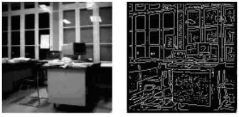
Edge detectors attempt to recover the discontinuities in the photometric, geomet-rical and physical characteristics of objects in the images. This information creates variations in the grey-level image. There are three steps to edge detection. The first step is noise smoothing to suppress as much of the image noise as possible, without destroying the true edges. The second step is edge enhancement, which means apply-ing a filter designed to be large at edge pixels and small elsewhere. The third step is edge localisation, which means deciding which local maxima in the filters output are edges and which are just caused by noise. Nonmaximum suppression to thin wide edges and thresholding can be used for edge localisation. There are three main ways to use the variation information, discontinuities (step edges), local extrema (line edges) and the 2D features formed where at least two edges meet [38]. Fig. 2.11 [30] shows an example of an original image and the position information provided by an edge detector. There are tens of edge detectors in the vision community, but they all produce similar results. Common edge detectors include Canny [39] and Sobel. Canny proposed the original edge detector in 1986, but it is still state-of-the-art today and still the most used.

focal length to improve stitching reliability, which finds corresponding edges for the matching. Edge detection is used in Bourque’s et al [42] work for determining inter-esting locations from where a robot should capture a spherical panorama.

Figure 2.11: Original image, and position information provided by edge detector

2.3.5 SIFT

Scale-invariant feature transform (SIFT), first proposed by Lowe in [49] and updated in [51] uses interest points (or keypoints) that have proved invariant to scale and rotation and robust to changes in viewpoint and illumination. The SIFT algorithm will be used for testing proposed methods against so is described here in more detail.

There are 4 main stages to the SIFT algorithm:

• Scale-space extrema detection

• Keypoint localisation

• Orientation assignment

• Keypoint descriptor

Scale-space extrema detection

Candidate keypoints are detected using a Gaussian based cascading filtering approach. Candidate locations are compared across different scale-spaces [52] to find points that are invariant to scale changes. Convolution of a variable scale Gaussian filter with an image produces multiple scales of an image. Adjacent scales are compared using a difference-of-Gaussian function. This subtracts one scale space image from another. Once multiple d-o-G images are computed, possible delegates for keypoint selection are compared with their 8 neighbours, and 9 neighbours in the scale above and below. Stable keypoints are those which are either larger or smaller than all of the neighbours.

Keypoint localisation

reject points with a low contrast. Next poorly located edge points are rejected. Edges produce a strong response in the difference-of-Gaussian function. A poor edge point can be defined as having a large principle curvature across the edge, but a small one in the perpendicular direction. By applying a threshold to the ratio of the principle curves across and perpendicular to the edge, poor edge points can also be rejected.

Orientation assignment

Invariance to rotation can be acheived by assigning a consistent orientation to each keypoint. An orientation histogram is formed from the gradient orientations of key-points. Peaks in the orientation histogram correspond to dominant directions of local gradients. The highest peak on the histogram is used to determine orientation infor-mation. If there exists another peak within 80% of the highest then multiple keypoints are created, each with a different orientation.

Keypoint descriptor

The previous stages have provided a local 2D coordinate system in which to describe the local image region using keypoints with invariance to scale and orientation. This final stage computes a descriptor to provide invariance to illumination and viewpoint changes. The descriptor is formed from a vector based on orientation histograms taken from the surrounding pixels around a keypoint. The feature vector is also normalised to reduce the effects of global contrast and brightness changes, making the descriptor robust to lighting changes.

2.4 Colour Correction and Colour Constancy

diagonal model, shown in Eq. 2.4 which was adapted by Ives [53] and based on the theories of Von Kries.

of maximal reflectance for each of the R, G, and B bands.

A common approach to colour constancy is the use of the estimation illumination to correct the images to a canonical light. Finlayson et al [55] suggested that if a transform is linear, a diagonal model might be sufficient to model the colour transform. Generally colour cameras are tri-chromatic, which means in a colour image, each pixel is a 3 vector, one component per sensor channel and works independently. However, with increasing colour fidelity, more accurate transforms will be required [56].

Different linear colour transforms, where the colour variation may be caused by lighting, changes in viewpoint or capturing devices, are discussed as follows. The transform Matrix M across images I₁ and I₂ can be represented as

I₁∗M =I₂ (2.3)

1) Diagonal model

M = ⎡ ⎢ ⎢ ⎢ ⎢ ⎢ ⎣ α β γ ⎤ ⎥ ⎥ ⎥ ⎥ ⎥ ⎦ (2.4)

α= mean(R2)

mean(R₁) (2.5)

WhereR is the red channel image intensity values in the two images. β and γ are similar for green and blue channels.

General features:

• Simple, not accurate enough in some cases

• Based on greyworld principle and does not need matching geometric pixels in

the 2 images

M = ⎡ ⎢ ⎢ ⎢ ⎢ ⎢ ⎣

α α₁

β β₁

γ γ₁

⎤ ⎥ ⎥ ⎥ ⎥ ⎥ ⎦ (2.6)

α, β and γ will be the same as diagonal model. The offset can be obtained from polyfit in the individual channels.

General features:

• More accurate than diagonal model

• Two images require the same corresponding pixels

3) Linear model

M = ⎡ ⎢ ⎢ ⎢ ⎢ ⎢ ⎣

a b c

d e f

g h i

⎤ ⎥ ⎥ ⎥ ⎥ ⎥ ⎦ (2.7)

Where M can be computed by

M =I₁TI₁−1I₁TI₂ (2.8)

Where

I₁, I₂

is an [n,3] matrix and n is the number of pixels in the images. General features:

• Good accuracy

• Need the same corresponding pixels in both images

4) Linear model with affine M = ⎡ ⎢ ⎢ ⎢ ⎢ ⎢ ⎣

a b c a₁

d e f e₁

g h i i₁

⎤ ⎥ ⎥ ⎥ ⎥ ⎥ ⎦ (2.9)

In addition to equation 2.8, the offset can be obtained by

⎡ ⎢ ⎢ ⎢ ⎢ ⎢ ⎣ a₁ e₁ i_i ⎤ ⎥ ⎥ ⎥ ⎥ ⎥ ⎦ = ⎡ ⎢ ⎢ ⎢ ⎢ ⎢ ⎣

mean(R₂)

mean(G₂)

mean(B₂)

⎤ ⎥ ⎥ ⎥ ⎥ ⎥ ⎦− ⎡ ⎢ ⎢ ⎢ ⎢ ⎢ ⎣

a b c

d e f

g h i

⎤ ⎥ ⎥ ⎥ ⎥ ⎥ ⎦× ⎡ ⎢ ⎢ ⎢ ⎢ ⎢ ⎣

mean(R₁)

mean(G₁)

mean(B₁)

⎤ ⎥ ⎥ ⎥ ⎥ ⎥ ⎦ (2.10)

The general features are the same as the linear model.

As described above, to obtain better colour correction, more parameters in lin-ear transforms will be used. We will use and compare diagonal model plus affine transform, linear model and linear model plus affine for colour correction in image correction for panoramic imaging.

2.5 Image Mosaicing and 3D Reconstruction

For panoramic imaging the images that have gone through image processing need to be mosaiced, or stitched, together.

For 3D reconstruction, the stereo images are used to calculate the disparity be-tween the image data.

2.5.1 Mosaicing

The creation of panoramic images and mosaics from a video sequence or a collec-tion of images has attracted tremendous attencollec-tion from researchers and commercial practitioners alike. Most systems for creating panoramas require the use of special fixtures (e.g. tripods and rotators) for precisely controlled image capture [57] and are transformed by their geometrical mapping [58].

In the last few years general interest in mosaicing has proliferated the vision and graphics community because of the range of possible applications i.e. teleconfer-encing, e-commerce, reconstruction of virtual environments and games. Szeliski et al have presented techniques for automatically deriving realistic 2D scenes and 3D texture mapping models from video sequences with applications in virtual environ-ments [58, 59, 60]. The principal task in image mosaicing is finding the corresponding points and their transforms from the source images, especially when the stitching images have been produced in different capture conditions with different viewpoints and capture devices. One of the approaches is to compute eigenimage features using principal component analysis (PCA) for finding corresponding areas [61]. Another approach applies wavelet-based edge preserving for finding corresponding image fea-tures [40]. However, edge-based feafea-tures are not robust to viewpoint changes. Also recent progress on pattern recognition, based on local features, invariant features in particular, has been used in many applications [49]. Interest points have been extensively investigated for object recognition and content-based image retrieval in computer vision [49, 62, 63] and corner-based image mosaicing has been presented with reasonably good results [46]. The SIFT algorithm has proven very robust and popular as a correspondence search and matching method for panoramic imaging and object recognition.

or a collection of images of a 3D scene taken from the same point of view, the only difference between the images is a rotation around the optical center of the camera and the transformation between the images is a linear transformation of projective space, called a collineation or a homography [64]. Previous work simplifies 2D image mosaics by the homography estimation [33]. Two cases have been investigated. The first is when the homography is mainly a translation and the rotation around the optical axis and zooming are small. The second is the general case where the rotation around the optical axis and zooming are large. Some efficient methods have been developed to handle the first case. For example, if the overlap of the images is very large, it has been shown that a non linear criterion minimization using the Levenberg-Marquardt method yields very good results [58], but it is very sensitive to the local minima and computationally expensive. A corner-based method to compute the homography between two images with small overlap (around 50%) and arbitrary rotation around the optical axis has been presented and used to build a 2D mosaic from a set of images [46, 65]. For 3D object images, a precise imaging mosaic has exploited non-linear transforms, for example the quadratic transform [65, 66]. This is the second-order Taylor expansion of the general interframe mapping function where the usual affine transformation model is the first-order expansion.

As described above, previous work to date mainly concentrated on geometric trans-formations for image mosaics. With the wide use of colour imaging, spectral transfor-mation is also becoming important, particularly for dealing with image mosaics under various conditions. Colour image transformation and correction for illumination can apply linear models [67, 56]. The diagonal model plus affine transform will be used in this work.

devices into larger, faster, more efficient arrays stimulates technological developments in both the hardware and software aspects of imaging techniques. Improvements in identification and recognition have long been recognised as the primary goals of intelligent systems. The motivation for this work is the many potential applications in teleconferencing, construction of image-based virtual environments, e-commerce, medical imaging and panoramic imaging.

For panoramic stitching or mosaicing, the features that are found in the previous methods are then used to calculate the homograph between the two images. The homograph is a mapping between two perspective images of a planar surface in a scene [68, 69]. In effect this means that two images of a scene are related by a homograph, typically a 3x3 matrix (see eq. 2.11). This homograph can be used to re-map images onto different planes.

λ ⎡ ⎢ ⎢ ⎢ ⎢ ⎢ ⎣ x y 1 ⎤ ⎥ ⎥ ⎥ ⎥ ⎥ ⎦ = ⎡ ⎢ ⎢ ⎢ ⎢ ⎢ ⎣

H_1,1 H_1,2 H_1,3

H_2,1 H_2,2 H_2,3

H_3,1 H_3,2 H_3,3

⎤ ⎥ ⎥ ⎥ ⎥ ⎥ ⎦ ⎡ ⎢ ⎢ ⎢ ⎢ ⎢ ⎣ x y 1 ⎤ ⎥ ⎥ ⎥ ⎥ ⎥ ⎦ (2.11)

such as the one in Fig. 2.14. The image in Fig. 2.14 used a homographic matrix to align the images from Fig. 2.12 and Fig. 2.13 correctly after the ’best fit’ matrix was computed from feature points in the images. Then colour correction algorithms were applied to create the final image, shown in 2.15. Mann and Picard [70] use video sequences and mosaicing to build high resolution images, and Kourogi et al [71] have created a real time mosaicing system using video sequences. Zhu et al [72] use video mosaics for stereo imaging.

Figure 2.12: Left original image before the mosaicing

Figure 2.13: Right original images before the mosaicing

Figure 2.14: Two images stitched together (without blending)

Figure 2.15: Two images stitched together (with blending)

or more images into a larger mosaic. In this technique the images are used as a set of band-pass filtered component images, instead of using the whole image data. Onoe et al [74] use omni directional video streams to create real-time view-dependent perspective images, which lends itself to real-time telepresence systems.

2.5.2 3D Construction

reconstruc-tion attempts to recover the 3D scene from this 2D version. It is the well-known ill-posed computer vision problem. Particularly, the reconstruction of a dynamic, complex 3D scene from multiple images is an old and challenging problem. Early work by Longuet-Higgins [75] into deriving 3D information from 8 points led the way for 3D reconstruction and his work is still the basis for many of todays algorithms. Numerous studies have been conducted on various aspects of this general problem, such as the recovery of the epipolar geometry between two stereo images, the calibra-tion of multiple camera views, stereo reconstruccalibra-tion by solving the correspondence problem, the modelling of the occlusions, the fusion of stereo and motion, and the fu-sion of multiple images by lighting variation [76]. Of course the most accurate method of 3D reconstruction is to use Laser measurement. This can be expensive and where people are included in the panoramic scene a risk to health exists. Yu et al [77] used a laser mounted on a van to produce accurate models of road surfaces and a video camera to produce the texture.

Figure 2.16: 3D surface reconstruction

information from different sources such as stereo vision, video sequences or multiple images under different lighting are input for feature extraction. The feature extraction will obtain point, edge, area, colour, texture features etc for matching corresponding features in different image resources. Then depth estimation will calculate the depth information for 3D data and visualisation. Many approaches have been investigated in the last few decades. More details are discussed in the following paragraphs.

Using the correspondence information, a disparity map can be computed, as illus-trated in Fig. 2.17 [78]. The disparity is the distance between corresponding pixels, and can be used to triangulate the 3D position of the pixels in the image. One of the biggest problems in stereo imaging, apart from correspondence, is the problem of occlusions. Stereo imaging uses multiple views of the same scene, either with the same camera from different viewpoints, or with multiple cameras. There are many ways of calculating the disparity from stereo images, including using structured light, geometry based approaches, image based approaches and parallax based approaches. Dhond and Aggarwal [76] reviewed the state-of-the-art techniques up until 1989 in their paper, which this section continues. Park and Inoue [79] use multiple cameras to capture information, and use the information in a hierarchical depth mapping system to overcome the occlusion problem. Hamden et al [80] use a trinocular vision sys-tem together with structured light to create a fast 3D object reconstruction syssys-tem. Valkenburg and McIvor [81] use a single camera with a projector which projects a stripe pattern onto the object which the camera captures.

views of the scene can be calculated. Izquierdo and Kruse [85] use stereo imaging for calculating arbitrary views of the extracted models. Lee et al [86] use a similar approach to stereo, using a front, back and side image, to create human models from photographs. The system uses interest points to determine the silhouette of the hu-man. Sietz and Dyer [87] use two images in a similar way to stereo vision, but they use them to generate physically valid synthetic views of the scene, in effect viewing the scene from a different viewpoint, not captured in the original images. Debevec et al [88] approach the model generation technique from a different angle. They use a manual photogrammetric method for the initial simple model, and then use a model based stereo algorithm, which recovers how the real scene differs from the model. This technique is limited to architectural models though, because it uses constraints that are characteristic of architectural scenes. Oh et al [89] use a single image, with much user input to generate 3D models. The system relies on the users input for assigning layers, and depths. Aliaga and Carlbom [90] use multiple panoramas to create a new walkthrough of a large environment. Their system captures the panoramas and uses them to plot a series of interlocking ”walkways”, which can be used to generate the new walkthroughs.

Figure 2.17: Stereo images and related disparity map

image from all the items such as pixels, edges, regions and objects in the left image [92, 93, 99]. The correspondence problem is commonly calculated with either area-based [100, 101, 24] or feature-area-based [92, 94, 102] methods. Feature area-based methods use features such as edges or points, like corners. Area based methods use neighbour-hoods around the pixel being computed. The reconstruction problem needs additional information about the cameras and assumptions about the scene and uses them to estimate disparities between items [94, 103, 104, 105]. To reduce the searching time of finding corresponding items, one well-known constraint is the epipolar constraint [99] as illustrated in Fig. 2.18. A point in an image creates an epipolar line on which the corresponding point in the other image must lie. Fig. 2.18 shows an example of a 3D pointP, the two camera locationsOl andOrand the pointmlwith its corresponding pointmr. The lineer andelare the epipolar lines and the plane formed by the points

Figure 2.18: Epipolar geometry and epipolar plane

Epipolar geometry means a previous 2D search for corresponding points now be-comes a 1D search, which as well as being much faster also means fewer false or ambiguous matches. This constraint to the correspondence search is called the epipo-lar constraint. In order to determine the epipoepipo-lar line from a point in an image the essential matrix and the fundamental matrix must be calculated. The essential matrix defines the relationship between an image point defined in camera coordinates and the epipolar line. The fundamental matrix defines the relationship between an image point defined in pixel coordinates and the epipolar line. The essential matrix can be computed using three vectors that lie on the epipolar plane,P_l, T and (P_l−T). The epipolar plane is computed by

(P_l−T)T (T ×P_l) = 0→RTP_rT (T ×P_l) = 0 (2.12)

Where T×P_l (cross product) is a vector perpendicular to the plane containingT and

P_l (the epipolar plane). P_l−T is also in the same plane, so the dot product is zero. The cross product can be written as

T ×P_l =SP_l→S =

⎡ ⎢ ⎢ ⎢ ⎢ ⎢ ⎣

0 −T_z T_y

T_z 0 −T_x

−T_y T_x 0

From 2.12 and 2.13 we getP_rTEP_l= 0 →E =RS where matrixE is the essential matrix which defines the epipolar constraint in terms of the extrinsic parameters. More computation about epipolar constraints for stereo vision can be found in [99, 106]. As a basic constraint, many researchers have used the epipolar constraint for reducing search time [92]. Other constraints are also possible, for example the use of rigidity constraints [107].

Following the corresponding points process, depth information can be calculated, by using triangulation as illustrated in Fig.2.19. Triangulation is the process of de-termining the position of a point in a scene if that point is visible in two images [103]. Triangulation needs information about the camera for correct results, these are the focal length of the camera and the distance between the camera positions, or baseline, when the images were captured. These intrinsic camera properties can be found using camera calibration techniques. Suppose a point P is visible in two images. If the two camera matrices are known, the points ml and mr are projections of the point P in the two images. From the available data the two rays in space corresponding to the two image points may easily be computed [103]. The triangulation problem is to find the intersection of the two lines in space. For example to find theZ value of the point

P (X, Y, Z). The corresponding points in the images are of the form ml(x1, y1) and its matching point mr(x2, y2) where the pointmr in the right image corresponds to the point mlin the left image. In this example the disparity is on the x axis only (for example if the corresponding points were on all the epipolar lines and the images were corrected). If the focal length of the camera is f, y1 = y2 and the distance between the cameras is b then the 3D point P(X, Y, Z) can be computed by the equation 2.14. The intrinsic and extrinsic parameters of the cameras need to be calibrated or modelled [104, 105, 108].

Z = f b

x2−x1 (2.14)

ex-Figure 2.19: Triangulation to find a point in 3D from 2 2D images

pair of cameras are available to capture binocular image sequences [119]. Recently a few researchers have extended stereo imaging with panoramic imaging to create stereo panoramic imaging [120, 23, 25, 102, 121, 24], which lends itself to creating 3D environments of the real world.

2.5.3 Stereo Panoramas

2.5.4 Rendering and 3D visualisation

based rendering have many complimentary characteristics, and in the future hardware should be designed for both. Kiyokawa et al [128] use an optical see-through display for mutual occlusion with a real-time stereovision system. This enables 3D objects to be integrated with video in real-time.

2.6 Discussions

Panoramic or omni-directional cameras allow the opportunity to capture rich data about an environment that can then be used to generate ”walk-throughs” for VR, or backgrounds for games, or tourism [12]. The panoramic imaging system is a typical system using the convergence of computer vision and computer graphics as described above. Computer graphics and computer vision could be described as taking op-posite approaches to the same problems. Computer vision develops novel capture techniques while computer graphics adopts techniques from computer vision for cap-turing models from the real world and also for reconstructing movement for virtual worlds. However, traditional view computer graphics start with inputting geometric models and producing image sequences whereas computer vision starts with inputting image sequences and producing geometric models, at least as an intermediary step. Linking with the real world, the virtual world is based on 3D, which will drive cur-rent panoramic imaging systems from 2D to 3D including hardware and software. The nucleation of virtual reality, graphics, video and vision is predicted to be an impor-tant area of research, particularly for 3D panoramic imaging and virtual environment construction. Some challenges exist in the following areas.

2.6.1 Stereo Vision Based Panoramic Capture System

the problem of automatically recovering useful surface or image-based models from this data for stereo panoramic imaging. Instead of using special equipment, 3D scenes obtained from stereo vision can be easily visualised in a VR environment. Equally, the viewed scene can be changed based on different viewpoints and other view conditions. A very interesting and exciting application of mixing stereo and panoramic imaging is the Beagle 2 Stereo camera system [129]. Unfortunately it was never used on Mars, but they integrated stereo imaging for digital elevation models and parabolic mirrors for panoramic imaging into a single system. Video based reconstruction techniques must be developed which allow a user to interactively recover models of a scene and select viewpoints (much like a video paint brush that allows a user to interactively recover representations of the scene).

2.6.2 Deriving Capturing Conditions and Object Surface Characteristics

Image formation on a digital sensor integrates illumination information and object surface characteristics within the visible spectrum. It would be useful to reverse the capture device, illumination and scene surface characteristics from the captured data. For example, colour constancy algorithms have provided some approaches to estimate the illuminant of an image. Based on the illumination, linear models, particularly the diagonal model can be used for colour correction and transformation [130] where lighting or viewpoints are changed.

2.6.3 Image Understanding and 3D Reconstruction

concerned with enabling a human operator to conduct tasks more effectively in a remote or hazardous environment when using a telepresence interface. Since vision is central to comprehending the remote environment, the main AR technique is to over-lay computer generated graphical information upon the operator’s view of the real scene [128]. Thus, it is possible to provide additional qualitative and quantitative information to the operator. In the latter case, the real and graphical worlds must be made to register, or correspond, with each other statically or dynamically depending on the application. Registration is required whenever quantitative information needs to flow between the real and graphical worlds and is a key element of most applica-tions. It requires careful calibration and modelling of all the real world sensors into the graphical world. The sensor data is used to update the graphical model, often in real-time, using transformation matrices. Inaccuracies in the sensor data and the ma-trices gives rise to a dynamic registration error between the two worlds that manifests as a jerky or swimming motion for the overlaid graphics. Some invariant features for registration or correspondence, which are robust to image capturing condition and devices, will be a future research direction [130]. Video research is an evolution of vision and graphics work. The number of images is large and increasing bringing a need for greater compression. While it is good to have fewer samples, this does not guarantee fewer bits. If a sequence of images is seen as a video sequence, then general video coding can be applied, however, this intra-coding does not exploit the correlation between images. The use of intracoding however does not provide random access (i.e. frame N depends on frame N-1).

2.6.4 Image Based Volumetric Rendering

the difficult and labour-intensive processes of traditional model construction. Critical to image-based modelling and rendering of virtual environments, and image-based animation of virtual objects, are compression and decompression of the large amount of visual data. There is also no current work integrating virtual character animation with IBR, although on the horizon are hybrid representations that use both geometric models and IBR that will allow greater flexibility in dynamics. Also the integration of IBR with video needs to be addressed to add dynamic surface appearance. Volumetric reconstruction from multiviews is now quite well understood and analysed. The main difficulties remain in turning the volumetric representation into a model and/or IBR form and in extracting a representation of surface appearance properties to allow realistic rendering for 3D panoramas.

2.6.5 Problems identified

In this chapter the different stages of panoramic imaging and stereo vision techniques have been discussed. Major advances in digital imaging and vision computing have been reviewed. These reviews suggest direction for future research. 3D panoramic imaging will be a feasible approach for fast, realistic virtual environment construction. From the literature survey it was determined that the work should concentrate on several issues.

The first is the problem of colour constancy. When moving the camera to capture the next image in a panoramic sequence changes in the lighting and/or camera settings (automated) means that sequential images can have different appearances. Making sure the images are as similar as possible in colour and lighting is important for successful mosaicing.

corre-spondences are required and can be taken from areas where probability of a successful match will be high.

Chapter 3

THEORY AND PROJECT ISSUES

3.1 Project concept and major elements

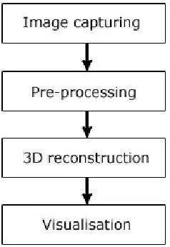
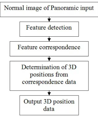
The basic theory of this project is to develop algorithms for areas within the process of creating 3D from 2D. The work concentrates on several small elements of the whole process. The project areas include the capture of the digital images, the pre-processing of the images, the 3D reconstruction and visualisation, as shown in Fig. 3.1.

Figure 3.1: The basic theory of the project

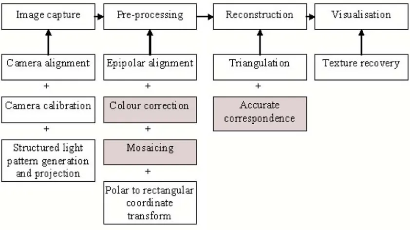
the alignment problem and printed patterns used to achieve accurate focusing. The pre-processing includes epipolar alignment, colour correction, accurate mosaicing us-ing homography and coordinate transform for the ’one-shot’ mirror system. 3D re-construction includes triangulation and accurate correspondence. For visualisation accurate texture recovery is required. Fig. 3.2 shows a more complete picture of the process, with each sub element shown under the main project stages. The shaded components are the areas this work addresses.

Figure 3.2: Showing the sub elements within each stage of the project

3.2 Key project elements

3.2.1 Image capture

Within the capture element accurate alignment of the cameras and camera calibra-tion is required. Without accurate initial capture informacalibra-tion the later stages will contain errors. It is important to ensure accurate capture by checking the alignment with templates, and camera calibration using a known calibration pattern, captured several times and used to calculate the camera properties. In the project two cap-ture systems are available. One system is based on a high resolution digital SLR camera with a 0-360.com ’one-shot’ parabolic mirror attached. This system enables the capture of panoramic images in a single image. The other system is a modular system. The modular system is able to capture stereo vision images, for example for object or face reconstruction, and also capture multiple images for mosaicing into a single panorama. This second system uses low resolution web cameras. The use of web cameras keeps the project costs to a minimum with the goal of proving accurate depth information can be achieved with low cost low resolution equipment. Camera calibration is only required for the second capture system. For example when recon-structing small objects using stereo vision, or capturing multiple images for mosaicing, camera calibration is required to determine the intrinsic and extrinsic parameters of the cameras. Another element of the capture phase is a structured light pattern. This pattern is used to assist the correspondence search algorithm by increasing the texture in areas of low texture, for example walls. The structured light pattern needs to be of sufficient size and distribution to assist the correspondence search, but also suitable for filtering for later texture recovery.

3.2.2 Pre-processing