Selection of Optimal Lag Length in
Cointegrated VAR Models with Weak
Form of Common Cyclical Features
Carrasco Gutierrez, Carlos Enrique and Castro Souza,
Reinaldo and Teixeira de Carvalho Guillén, Osmani
2009
Online at
https://mpra.ub.uni-muenchen.de/66065/
Cointegrated VAR Models with Weak
Form of Common Cyclical Features
*Carlos Enrique Carrasco Gutierrez**
Reinaldo Castro Souza***
Osmani Teixeira de Carvalho Guill´en****
Abstract
An important aspect of empirical research based on the vector autoregressive (VAR) model is the choice of the lag order, since all inferences in this model depend on the correct model specification. There have been many studies on how to select the lag order of a nonstationary VAR model subject to cointegration restrictions. In this paper, we consider an additional weak-form (WF) restriction of common cyclical features in the model to analyze the appropriate way to select the correct lag order. We use two methodologies: the traditional information criteria (AIC, HQ and SC) and an alternative criterion (IC(p, s)) that selects the lag orderpand the rank structuresdue to the WF restriction. We use a Monte Carlo simulation in the analysis. The results indicate that the cost of ignoring additional WF restrictions in vector autoregressive modeling can be high, especially when the SC criterion is used.
Keywords: Cointegration, Common Cyclical Features, Reduced Rank Model, Information
Criteria.
JEL Codes: C32, C53.
*
Submitted in February 2009. Revised in August 2009. We are grateful for the comments and suggestions by Jo˜ao Victor Issler, Wagner Gaglianone, Ricardo Cavalcanti, Luiz Renato Lima and many seminar participants at the 2006 Brazilian Econometric Meeting and 2007 European Econometric Meeting in Hungary. We extend special thanks to Alain Hecq for solving doubts and providing helpful comments. We are responsible for any remaining errors in this paper. Carlos Enrique also acknowledges financial support from Getulio Vargas Foundation and CAPES (Coordination for the Improvement of Higher Level Personnel).
**
FUCAPE Business School, Vit´oria, Brazil. E-mail: [email protected]
***
DEE-PUC-RJ, Brazil. E-mail: [email protected]
****
1. Introduction
In the modeling of economic and financial time series, the vector autoregressive (VAR) model has become the standard linear model used in empirical works. An important aspect of empirical research on the specification of VAR models is determination of the lag order of the autoregressive lag polynomial, since all inferences in the VAR model depend on the correct model specification. Several works have demonstrated the effect of lag length selection. L¨utkepohl (1993) indicated that selecting a higher order lag length than the true one causes an increase in the mean square forecast errors of the VAR and that underfitting the lag length often generates autocorrelated errors. Braun and Mittnik (1993) showed that impulse response functions and variance decompositions are inconsistently derived from the estimated VAR when the lag length differs from the true length. When cointegration restrictions are considered in the model, the effect of lag length selection on the cointegration tests has been demonstrated. For example, Johansen (1991) and Gonzalo (1994) pointed out that VAR order selection can affect proper inference about cointegrating vectors and rank.
Recently, empirical works have considered other kinds of restrictions in the VAR model (e.g., Engle and Issler (1995); Caporale (1997); Mamingi and Iyare (2003)). Engle and Kozicki (1993) showed that VAR models can have other types of restrictions, called common cyclical features, which are restrictions on the short-run dynamics. These restrictions are defined in the same way as cointegration restrictions, but while cointegration refers to relations among variables in the long run, common cyclical restrictions refer to relations in the short run. Vahid and Engle (1993) proposed the serial correlation common feature (SCCF) as a measure of common cyclical features. SCCF restrictions might be imposed in a covariance stationary VAR model or in a cointegrated VAR model. The concept of serial correlation common features appears to be useful. It means that stationary time series move together in a way such that there are linear combinations of these variables which yield white noise processes and that their impulse response functions are collinear. In several practical applications the existence of short-run comovements between stationary time series (e.g., between first-differenced cointegrated I(1)) has been analyzed. For instance, Engle and Issler (1995) found common cycle comovement in U.S. sectoral output data; Hecq (2002) and Engle and Issler (1993) found common cycles in Latin American countries; and Carrasco and Gomes (2009) found common international cycles in GNP data for Mercosur countries.
of the vector error correction model (VECM).1 When SCCF are imposed, all matrices of a VECM have rank less than the number of variables analyzed. On the other hand, with WF restrictions, all matrices except the long-run matrix have rank less than the number of variables being analyzed. Hence, WF restrictions impose less constraint on VECM parameters. Some advantages emerge when WF restrictions are considered. First, due to the fact that the weak-form common cyclical method does not impose constraints on the cointegration space, the rank of common cyclical features is not limited by the choice of cointegrating rank.
The literature has shown how to select an adequate lag order of a covariance stationary VAR model and an adequate lag order of a VAR model subject to coin-tegration restrictions. Among the classical procedures are information criteria, such as Akaike (AIC), Schwarz (SC) and Hannan-Quinn (HQ) (L¨utkepohl, 1993). Kilian (2001) studied the performance of traditional AIC, SC and HQ criteria of a covariance stationary VAR model. Vahid and Issler (2002) analyzed the standard information criteria in a covariance stationary VAR model subject to SCCF re-striction and, more recently, Guill´en et al. (2005) studied the standard information criteria in VAR models with cointegration and SCCF restrictions. However, when cointegrated VAR models contain an additional weak form of common cyclical features, there are no reported works on how to appropriately determine the VAR model order.
The objective of this paper is to investigate the performance of information criteria in selecting the lag order of a VAR model when the data are generated from a true VAR with cointegration and WF restrictions, referred to as the correct model. We carry out the following two procedures:
a) the use of standard criteria, as proposed by Vahid and Engle (1993), referred to here as IC(p), and
b) the use of an alternative model selection criterion (see Vahid and Issler (2002) and Hecq et al. (2006)), which consists in simultaneously selecting the lag orderpand the number of weak forms of common cyclical features,s, which is referred to as IC(p, s).2
The most relevant results can be summarized as follows. The information criterion that selects the pair (p, s) performs better than the model chosen by conventional criteria, especially the AIC(p, s) criterion. The cost of ignoring additional WF restrictions in vector autoregressive modeling can be high, particularly when the SC(p) criterion is used.
The rest of this paper is organized as follows. Section 2 presents the economet-ric model. Section 3 discusses the information criteria. Section 4 shows a Monte
1
When a VAR model has cointegration restriction it can be represented as a VECM. This representation is also known as Granger representation theorem (Engle and Granger, 1987).
2
Carlo simulation and Section 5 presents the results. Finally, Section 6 contains our conclusions.
2. The Econometric Model
We show the VAR model with short-run and long-run restrictions. First, we consider a Gaussian vector autoregression of finite order p, called VAR(p), such that:
yt= p
X
i=1
Aiyt−i+εt (1)
where, yt is a vector of n first-order integrated series, I(1), Ai, i = 1, . . . , pare
matrices of dimension n×n, εt ∼N ormal(0,Ω), E(εt) = 0 and E(εtε
′
τ) ={Ω
, if t = τ and 0n×n, if t 6= τ, where Ω is nonsingular}. The model (1) can
be written equivalently as; Π (L)yt = εt where L represents the lag operator
and Π (L) = In−P p
i=1AiLi such that when L = 1, Π (1) = In −P p
i=1Ai. If
cointegration is considered in (1) the (n×n) matrix Π (·) satisfies two conditions: a) rank (Π (1)) = r, 0 < r < n, such that Π (1) can be expressed as Π (1) =
−αβ′
, where αand β are (n×r) matrices with full column rank, r; and b) the characteristic equation|Π (L)| = 0 has n−r roots equal to 1 and all others are outside the unit circle. These assumptions imply that yt is cointegrated of order
(1,1). The elements of α are the adjustment coefficients and the columns of β
span the space of cointegration vectors. We can represent a VAR model as a vector error correction model (VECM). By decomposing the polynomial matrix Π (L) = Π (1)L+ Π∗
(L) ∆, where ∆≡(1−L) is the difference operator, a VECM is obtained:
∆yt=αβ
′
yt−1+
p−1 X
i=1
Γi∆yt−i+εt (2)
where: αβ′
=−Π (1), Γj =−Ppk=j+1Ak for j = 1, ...., p−1 and Γ0=In. The
VAR(p) model can include additional short-horizon restrictions as shown by Vahid and Engle (1993). We consider an interesting WF restriction (as defined by Hecq et al. (2006)) that does not impose constraints on long-run relations.
Definition 1 The weak form (WF) holds in (2) if, in addition to cointegration restriction, there exists an (n×s) matrix β˜ of rank s, whose columns span the cofeature space, such thatβ˜′
(∆yt−αβyt−1) = ˜β′εt, whereβ˜
′
εtis ans-dimensional
Equivalent to Definition 1, we consider WF restrictions in the VECM if there exists a cofeature matrix ˜β that satisfies the following assumption:
Assumption 1: β˜′
Γj= 0s×n for j= 1, ...., p−1.
Therefore, this is a naturally weaker alternative assumption which implies that the common cyclical part is reduced to white noise by taking a linear combination of the variables in the first differences adjusted for long-run effects. Imposing WF restrictions is convenient because it allows for the study of both cointegration and common cyclical feature without the constraint3 r+s≤n.
We can rewrite the VECM with WF restrictions as a model of reduced-rank structure. In (2) letXt−1= [∆y′t−1, ...∆y
′
t−p+1]
′
and Φ = [Γ1, ....,Γp−1].
There-fore, we obtain:
∆yt=αβyt−1+ ΦXt−1+εt (3)
If Assumption (1) holds, then matrices Γi, i= 1, ..., pare all of rank (n−s) and
we can write Φ = ˜β⊥Ψ = ˜β⊥[Ψ1, ....,Ψp−1], where, ˜β⊥ isn×(n−s) full column
rank matrix, Ψ has dimension (n−s)×n(p−1),and the matrices Ψi, i= 1, ..., p−1
all have rank (n−s)×n. Hence, given Assumption (1), there exists ˜β of n×s
such that ˜β′˜
β⊥= 0. That is, ˜β⊥ n×(n−s) is a full column rank orthogonal to
the complement of ˜β withrank( ˜β,β˜⊥) =n. Rewriting model (3) we have:
∆yt=αβyt−1+ ˜β⊥(Ψ1,Ψ2, ...,Ψp−1)Xt−1+εt (4)
=αβyt−1+ ˜β⊥ΨXt−1+εt (5)
Estimation of (5) is carried out via the switching algorithms (see Centoni et al. (2007); Hecq (2006)) that use the procedure in estimating reduced-rank regression models as suggested by Anderson (1951). There is a formal connection between a reduced-rank regression and the canonical analysis, as noted by Izenman (1975), Box and Tiao (1977), Tso (1981) and Velu et al. (1986). When all the matrix coefficients of the multivariate regression are full rank, they can be estimated by the usual least squares or maximum likelihood procedures. But when the matrix coefficients are of reduced rank they have to be estimated using the reduced-rank regression models of Anderson (1951). The use of canonical analysis may be regarded as a special case of reduced-rank regression. More specifically, the maxi-mum likelihood estimation of the parameters of the reduced-rank regression model may solve a problem of canonical analysis.4 Therefore, we can use the expression
CanCorr{Xt, Zt|Xt−1} which denotes the partial canonical correlations between
3
Since the SCCF also imposes constraints on the long-run matrixαβ′=−Π (1), which has
dimensionn, the cointegration restrictions,r, and SCCF restrictions,s, must satisfyr+s≤n.
4
Xt and Zt: both sets are concentrated out of the effect ofXt−1 allowing us to
obtain canonical correlation (see Johansen (1995)), represented by the eigenvalues ˆ
λ1 >λˆ2>ˆλ3... >λˆn. The Johansen test statistic is based on canonical
corre-lation. In model (2) we can use the expressionCanCorr{∆yt, yt−1|Xt−1} where
Xt−1= [∆y′t−1, ...∆y
′
t−p+1]
′
, which summarizes the reduced-rank regression pro-cedure used in Johansen approach. This means that we extract the canonical correlations between ∆ytandyt−1: both sets are concentrated out of the effect of
lags of Xt−1. In order to test for the significance of the r largest eigenvalues, we
can rely on Johansen’s trace statistic (6):
ξr=−T n
X
i=r+1
Ln(1−λˆ2i) i= 1, ..., n (6)
where the eigenvalues 0 < λˆn < ... < λˆ1 are the solution to : |λm11 −
m−1
10m00m01| = 0, where mij, i, j = 0.1, are the second-moment matrices:
m00 = T1PTt=1u˜0tu˜
′
0t, m10 = T1 PTt=1u˜1tu˜
′
0t, m01 = T1 PTt=1u˜0tu˜
′
1t, m11 = 1
T
PT
t=1u˜1tu˜
′
1t of the residuals ˜u0t and ˜u1t obtained in the multivariate least
squares regressions ∆ yt = (∆yt−1,...,∆yt−p+1) +u0t and yt−1 = (∆yt−1, ...
∆yt−p+1) +u1t respectively (see, Hecq (2006); Johansen (1995)). The result of
Johansen test is a superconsistent estimation ofβ. Moreover, we could also use a canonical correlation approach to determine the rank of the common feature space due to WF restrictions. This is a test for the existence of cofeatures in the form of linear combinations of the variables in first differences, corrected for long-run effects which are white noise (i.e., ˜β′
(∆yt−αβyt−1) = ˜β′εtwhere ˜β
′
εt is a white
noise). We use canonical analysis is this work to estimate and select the lag rank of VAR models, as shown in the subsequent sections.
3. Model Selection Criteria
In model selection we use two procedures to identify the VAR model order: the standard selection criteria, IC(p), and the modified information criteria, IC(p, s), a novelty in the literature, which consists in identifyingpandssimultaneously.
The model estimation following the standard selection criteria, IC(p), originally used by Vahid and Engle (1993), entails the following steps:
1. Estimate p using standard information criteria: Akaike (AIC), Schwarz (SC) and Hanna-Quinn (HQ). We chose the lag length of the VAR in levels that minimizes the information criteria.
2. Using the lag length chosen in the previous step, find the number of cointegration vectors,r, using Johansen cointegration test.5
5
3. Conditional on the results of the cointegration analysis, estimate a final VECM and then calculate the multi-step ahead forecast.
The above procedure is followed when there is evidence of cointegration re-strictions. We check the performance of IC(p) when WF restrictions are imposed on the true model. Additionally, we check the performance of IC(p, s) alternative selection criteria. Vahid and Issler (2002) analyzed a covariance stationary VAR model with SCCF restrictions. They showed that the use of IC(p, s) performs better than IC(p) in VAR model lag order selection. In the present paper we an-alyze the cointegrated VAR model with WF restrictions in order to anan-alyze the performance of IC(p) and IC(p, s) for model selection. The question investigated is: Does IC(p, s) perform better than IC(p)? This is an important question we aim to answer in this paper.
The procedure to choose the lag order and the rank of the structure of short-run restrictions is carried out by minimizing the following modified information criteria (see Vahid and Issler (2002); Hecq (2006)).
AIC(p, s) =
T
X
i=n−s+1
ln(1−λ2i(p)) +
2
T ×N (7)
HQ(p, s) =
T
X
i=n−s+1
ln(1−λ2
i(p)) +
2 ln(lnT)
T ×N (8)
SC(p, s) =
T
X
i=n−s+1
ln(1−λ2i(p)) +
lnT
T ×N (9)
N = [n×(n×(p−1)) +n×r]−[s×(n×(p−1) + (n−s))]
wherenis the number of variables in model (2) andN is a number of parameters.
N is obtained by subtracting the total number of mean parameters in the VECM (i.e., n2×(p−1) +nr), for given r and p, from the number of restrictions the
common dynamics imposes froms×(n×(p−1))−s×(n−s). The eigenvalues
λi are calculated for eachp. In order to calculate the pair (p, s) we assume that
no restriction exists, that is, r = n (see Hecq (2006)). We fix p in model (3) and then find λi i = 1,2...n by computing the cancorr(∆yt, Xt−1 | yt−1). This
are inverting the hierarchical procedure followed by Vahid and Engle (1993) where the first step is to select the number of cointegration relations. This may be an advantage, especially whenris overestimated. Few works have analyzed the order of VAR models considering modified IC(p, s). As mentioned, Vahid and Issler (2002) suggested the use of IC(p, s) to simultaneously choose the order p and a number of reduced-rank structuresin a covariance stationary VAR model subject to SCCF restrictions. However, no work has analyzed the order of the VAR model with cointegration and WF restrictions using a modified criterion, which is exactly the contribution of this paper.
To estimate the VAR model, considering cointegration and WF restrictions, we use the switching algorithms model as considered by Hecq (2006). Consider the VECM given by:
∆yt=αβ
′
yt−1+ ˜β⊥ΨXt−1+εt (10)
A full description of switching algorithms is presented below in four steps:
Step1 : Estimation of the cointegration vectors β.
Using the optimal pair (¯p,¯s) chosen by the information criteria (7), (8) or (9), we estimate β (and so its rank, r = ¯r) using Johansen cointegration test.
Step2 : Estimation of ˜β⊥ and Ψ.
Taking the estimate ofβin step one, we proceed to estimate ˜β⊥and Ψ.
Hence, we run a regression of ∆ytand ofXt−1on ˆβ′yt−1. We label the
residualsu0andu1, respectively. Therefore, we obtain a reduced-rank
regression:
u0t= ˜β⊥Ψu1t+εt (11)
where Ψ can be written as Ψ = C1, ..., C( ¯p−1)
of (n−¯s)×n(¯p−1) and ˜β⊥ofn×(n−s¯). We estimate (11) by FIML. Thus, we can obtain
˜
β⊥ and ˆΨ.
Step3 : Estimation of the maximum likelihood (ML) function.
Given the parameters estimated in steps 1 and 2 we use a recursive algorithm to estimate the maximum likelihood (ML) function. We calculate the eigenvalues associated with ˆΨ, ˆλ2
i i = 1, ...,s¯ and the
matrix of residualsPmax ¯
r, s=¯s. Hence, we compute the ML function:
L0
max,r<n, s¯ =¯s=−
T
2
"
ln
max X
¯
r<n, s=¯s
−
¯
s
X
i=1
ln1−λˆ2
i
#
If ¯r = n, instead of (12) we use the derived log-likelihood:
Lmax, r=n, s=¯s = −T2 ln
Pmax ¯
r=n, s=¯s
. The determinant of the
covari-ance matrix for ¯r=ncointegration vector is calculated by
ln max X ¯
r=n, s=¯s
= ln
m00−m01m
−1 11m10
− ¯ s X i=1
ln1−λˆ2i
(13)
where mij refers to cross moment matrices obtained in multivariate
least squares regressions from ∆yt and Xt−1 on yt−1. In this case,
estimation does not entail using an iterative algorithm yet, because the cointegrating space spansRn.
Step4 : Reestimation ofβ.
We reestimateβ to obtain a more appropriate value for the parameters. In order to reestimateβwe compute theCanCorrh∆yt, yt−1|ΨˆXt−1
i
and thus using the new ˆβ we can repeat step 2 to reestimate ˜β⊥ and
Ψ. Then, we calculate the new value of the ML function in step 3. Hence, we obtain L1
max, r=¯r, s=¯s to calculate ∆L = (L1max, r=¯r, s=¯s
-L0
max, r=¯r, s=¯s).
We repeat steps 1 to 4 to choose ˜β⊥and Ψ until convergence is reached (i.e.,
∆L <10−7). In the end, the optimal parameters ¯p, ¯rand ¯sare obtained and they
can be used to estimate and forecast a VECM with WF restrictions.
4. Monte Carlo Design
The simple real business cycle models and also the simplest closed economy monetary dynamic stochastic general equilibrium models are three-dimensional. Consumption, saving and output and prices, output and money are notable ex-amples. Motivated by these applications and according to the previous paper of Vahid and Issler (2002), we construct a Monte Carlo experiment in a three-dimensional environment. Therefore, the data generating processes considering a VAR model with three variables, one cointegration vector, and two cofeature vectors (i.e.,n= 3,r= 1 and s= 2, respectively). β and ˜β satisfy:
β=
1.0 0.2
−1.0
,β˜=
1.0 0.1 0.0 1.0 0.5 −0.5
ε1t
ε2t
ε3t
∼N
0 0 0 ,
1.0 0.6 0.6 0.6 1.0 0.6 0.6 0.6 1.0
Consider the VAR(3) model: yt=A1yt−1+A2yt−2+A3yt−3+εt. The VECM
representation as a function of the VAR level parameters can be written as:
∆yt= (A1+A2+A3−I3)yt−1−(A2+A3)∆yt−1−A3∆yt−2+εt (14)
The VAR coefficients must simultaneously comply with the restrictions:
a) the cointegration restrictions: αβ′
= (A1+A2+A3−I3) ;
b) WF restrictions: ˜β′
A3 = 0 (iii) ˜β′(A2 +A3) = 0 and c) the covariance
stationary condition.
Considering the cointegration restrictions, we can rewrite (14) as the following VAR(1):
ξt=F ξt−1+vt (15)
ξt=
△yt
△yt−1
β′
yt
, F =
−(A2+A3) −A3 α
I3 0 0
−β(A2+A3) −β′A3 β′α+ 1
andvt=
εt
0
β′
εt
Thus, Equation (15) will be covariance stationary if all eigenvalues of matrix
F lie inside the unit circle. An initial idea to design the Monte Carlo experiment can consist in constructing the companion matrix (F) and verifying whether the eigenvalues of the companion matrix all lie inside the unit circle. This can be carried out by selecting their values from a uniform distribution, and then ver-ifying whether or not the eigenvalues of the companion matrix all lie inside the unit circle. However, this strategy could lead to a wide spectrum of search for adequate values for the companion matrix. Hence, we follow an alternative pro-cedure. We propose an analytical solution to generate a covariance stationary VAR, based on the choice of the eigenvalues, and then on the generation of the respective companion matrix. In the Appendix, we present a detailed discussion of the final choice of these free parameters, including analytical solutions. In our simulation, we constructed 100 data generating processes and for each of these we generated 1,000 samples containing 1,000 observations. To reduce the impact of the initial values, we considered only the last 100 and 200 observations. All the experiments were conducted in the MatLab environment.
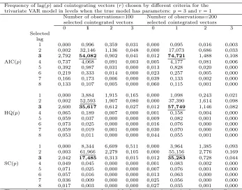
[image:11.595.47.396.235.297.2]5. Results
Figure 1 shows one example of the three-dimensional VAR model with cointe-gration and WF restrictions for 100 and 200 observations.
0 10 20 30 40 50 60 70 80 90 100 −10
0 10 20 30 40 50 60 70
Time Y1t
Y2t Y3t
0 20 40 60 80 100 120 140 160 180 200 10
20 30 40 50 60 70 80
Time Y1t
Y2t Y3t
[image:12.595.83.369.67.278.2]Figure 1
One example of a VAR(3) model withn= 3,r= 1 ands= 2 for 100 and 200 observations
happens when the weak-form common cyclical restrictions are ignored? Tables A.1 and A.2 also show the relative performance of IC(p, s) vis-`a-vis IC(p). For instance, forT = 100 the SC(p, s) has a success rate of 25.2% in selecting the true
p= 3, while the SC(p) only has a success rate of 17.48%. This represents a gain of more than 44%. ForT = 200, the gains are more than 27%. For T = 100 the HQ(p, s) selects the truep=3 witha 40.85% accuracy while the HQ(p) only has a success rate of 35.62%. This represents a gain of 14%. ForT = 200, the gains are more than 8%. For T = 100 the AIC(p, s) has a success rate of 56.34% in choosing the truep = 3, in comparison with a rate of 54.08% for the AIC(p), a gain of more than 4%. For T=200, the gains are more than 3%. Thus, it appears that when using the AIC(p,s) criteria the cost of ignoring the weak-form common cyclical restriction is low.
The most relevant results can be summarized as follows:
−All criteria (AIC, HQ and SC) choose the correct parameters more often when using IC(p, s) vis-`a-vis IC(p).
− There is a cost of ignoring additional weak-form common cyclical restrictions in the model especially when the SC(p) criterion is used. In general, the standard Schwarz, SC(p), or Hannan-Quinn, HQ(p), selection criteria should not be used for this purpose in small samples due to the tendency to identify an underparameterized model.
−The AIC performs better in selecting the true model more frequently for both the IC(p, s) and the IC(p) criteria.
6. Conclusions
In this paper, we considered an additional weak-form restriction of common cyclical features in a cointegrated VAR model in order to analyze the appropriate way to choose the correct lag order. These additional WF restrictions are defined in the same way as cointegration restrictions. While cointegration refers to relations among variables in the long run, the common cyclical restrictions refer to relations in the short run. Two methodologies have been used for selecting lag length; the traditional information criterion, IC(p), and an alternative criterion (IC(p, s)) that selects the lag order pand the rank structure s due to the weak-form common cyclical restrictions.
The results indicate that the information criterion that selects the lag length and the rank order performs better than the model chosen by conventional criteria. When the WF restrictions are ignored there is a nontrivial cost in selecting the true model with standard information criteria. In general, the standard Schwarz or Hannan-Quinn selection criteria should not be used for this purpose in small samples, due to the tendency to identify an underparameterized model.
provides considerable gains in selecting the correct VAR model. Since no work in the literature has analyzed a VAR model with WF common cyclical restrictions, the results of this paper provide new insights and incentives to proceed with this kind of empirical work.
References
Anderson, T. W. (1951). Estimating linear restrictions on regression coefficients for multivariate normal distributions.The Annals of Mathematical Statististics, 22:327–351.
Box, G. E. & Tiao, G. C. (1977). A canonical analysis of multiple time series.
Biometrika, 64:355–365.
Braun, P. A. & Mittnik, S. (1993). Misspecifications in vector autoregressions and their effects on impulse responses and variance decompositions. Journal of Econometrics, 59:319–41.
Caporale, G. M. (1997). Common features and output fluctuations in the United Kingdom. Economic Modelling, 14:1–9.
Carrasco, C. G. & Gomes, F. (2009). Evidence on common features and business cycle synchronization in Mercosur. Brazilian Review of Econometrics, 29:forth-coming.
Centoni, M., Cubadda, G., & Hecq, A. (2007). Common shocks, common dynamics and the international business cycle. Economic Modelling, 24:149–166.
Engle, R. & Granger, C. (1987). Cointegration and error correction: Representa-tion, estimation and testing. Econometrica, 55:251–76.
Engle, R. & Issler, J. V. (1993). Common trends and common cycles in Latin America. Revista Brasileira de Economia, 47:149–176.
Engle, R. & Issler, J. V. (1995). Estimating common sectoral cycles. Journal of Monetary Economics, 35:83–113.
Engle, R. & Kozicki, S. (1993). Testing for common features. Journal of Business and Economic Statistics, 11:369–395.
Gonzalo, J. (1994). Five alternative methods of estimating long-run equilibrium.
Journal of Econometrics, 60:203–233.
Hecq, A. (2002). Common cycles and common trends in Latin America. Medium Econometrische Toepassingen, 10:20–25.
Hecq, A. (2006). Cointegration and common cyclical features in VAR models: Comparing small sample performances of the 2-step and interative approaches. Mimeo.
Hecq, A., Palm, F. C., & Urbain, J. P. (2006). Testing for common cyclical features in VAR models with cointegration. Journal of Econometrics, 132:117–141.
Izenman, A. J. (1975). Reduced rank regression for the multivariate linear model.
Journal of Multivariate Analysis, 5:248–264.
Johansen, S. (1991). Estimation and hypothesis testing of cointegration vectors in Gaussian vector autoegressive models. Econometrica, 59:1551–1580.
Johansen, S. (1995). Likelihood-Based Inference in Cointegrated Vector Autore-gressive Models. Oxford University Press.
Kilian, L. (2001). Impulse response analysis in vector autoregressions with un-known lag order. Journal of Forecasting, 20:161–179.
L¨utkepohl, H. (1993). Introduction to Multiple Time Series Analysis. Springer, New York.
Mamingi, N. & Iyare, S. O. (2003). Convergence and common features in interna-tional output: A case study of the economic community of West African States 1975-1997. Asian African Journal of Economics and Econometrics, 3:1–16.
Tso, M. K. (1981). Reduced rank regression and canonical analysis. Journal of the Royal Statistical Society, 43:183–189.
Vahid, F. & Engle, R. (1993). Common trends and common cycles. Journal of Applied Econometrics, 8:341–360.
Vahid, F. & Issler, J. V. (2002). The importance of common cyclical features in VAR analysis: A Monte Carlo study. Journal of Econometrics, 109:341–363.
Appendix A: Tables
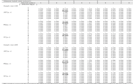
Table A.1 Performance of the IC(p) information criterion in selecting lag orderp
Frequency of lag(p) and cointegrating vectors (r) chosen by different criteria for the trivariate VAR model in levels when the true model has parameters:p= 3 andr= 1
Number of observations=100 Number of observations=200 selected cointegrated vectors selected cointegrated vectors
0 1 2 3 0 1 2 3
Selected lag
1 0,000 0,996 0,359 0,031 0,000 0,095 0,016 0,003
2 0,002 32,146 1,136 0,048 0,000 17,073 0,686 0,033
3 2,792 54,082 0,902 0,041 0,012 74,721 1,488 0,108
AIC(p) 4 0,737 4,068 0,091 0,003 0,005 4,177 0,081 0,006
5 0,392 0,987 0,031 0,000 0,013 0,828 0,020 0,000
6 0,219 0,333 0,014 0,000 0,023 0,257 0,005 0,000
7 0,166 0,173 0,006 0,000 0,039 0,133 0,002 0,000
8 0,133 0,107 0,005 0,000 0,060 0,115 0,001 0,000
1 0,000 3,884 1,915 0,165 0,000 1,098 0,243 0,021
2 0,002 52,593 1,907 0,080 0,000 37,390 1,614 0,098
3 2,600 35,617 0,612 0,027 0,012 57,749 1,146 0,082
HQ(p) 4 0,065 0,189 0,007 0,000 0,001 0,158 0,004 0,000
5 0,059 0,037 0,000 0,000 0,009 0,082 0,001 0,000
6 0,073 0,025 0,000 0,000 0,016 0,076 0,000 0,000
7 0,059 0,019 0,001 0,000 0,030 0,070 0,000 0,000
8 0,053 0,011 0,000 0,000 0,044 0,055 0,001 0,000
1 0,000 8,344 6,609 0,511 0,000 3,964 1,385 0,093
2 0,003 61,966 2,279 0,105 0,000 55,156 2,776 0,169
3 2,042 17,485 0,313 0,015 0,012 35,283 0,728 0,044
SC(p) 4 0,049 0,045 0,000 0,000 0,001 0,083 0,002 0,000
5 0,071 0,025 0,000 0,000 0,007 0,076 0,001 0,000
6 0,057 0,016 0,000 0,000 0,013 0,063 0,000 0,000
7 0,036 0,009 0,000 0,000 0,025 0,056 0,000 0,000
8 0,017 0,003 0,000 0,000 0,027 0,035 0,001 0,000
The numbers represent the percentage the model selection criterion has in choosing the cell corresponding to the lag and number of cointegration vectors in 100,000 runs.
rl o s E . C a rr a sc o G u ti e rr e z , R e in a ld o C a st ro S o u z a a n d O sm a n i T . d e C a rv a lh o G u ill ´e n
Selected rank(s) 1 2 3 1 2 3 1 2 3 1 2 3
Selected lag(p) Sample size=100
1 - - -
-2 0.002 0,000 0,000 39,049 0,001 0,000 1,218 0,000 0,000 0,056 0,000 0,000
3 0,301 0,000 0,000 56,341 0,003 0,000 1,559 0,000 0,000 0,053 0,000 0,000 AIC(p, s) 4 0,004 0,000 0,000 1,186 0,001 0,000 0,070 0,000 0,000 0,001 0,000 0,000 5 0,000 0,000 0,000 0,114 0,001 0,000 0,012 0,000 0,000 0,000 0,000 0,000 6 0,000 0,000 0,000 0,020 0,000 0,000 0,001 0,000 0,000 0,000 0,000 0,000 7 0,000 0,000 0,000 0,006 0,000 0,000 0,001 0,000 0,000 0,000 0,000 0,000 8 0,000 0,000 0,000 0,000 0,000 0,000 0,000 0,000 0,000 0,000 0,000 0,000
1 - - -
-2 0,002 0,000 0,000 55,563 0,000 0,000 1,888 0,000 0,000 0,081 0,000 0,000
3 0,267 0,000 0,000 40,855 0,000 0,000 1,207 0,000 0,000 0,043 0,000 0,000 HQ(p, s) 4 0,000 0,000 0,000 0,088 0,000 0,000 0,005 0,000 0,000 0,000 0,000 0,000 5 0,000 0,000 0,000 0,001 0,000 0,000 0,000 0,000 0,000 0,000 0,000 0,000 6 0,000 0,000 0,000 0,000 0,000 0,000 0,000 0,000 0,000 0,000 0,000 0,000 7 0,000 0,000 0,000 0,000 0,000 0,000 0,000 0,000 0,000 0,000 0,000 0,000 8 0,000 0,000 0,000 0,000 0,000 0,000 0,000 0,000 0,000 0,000 0,000 0,000
1 - - -
-2 0,004 0,000 0,000 70,971 0,000 0,000 2,574 0,000 0,000 0,113 0,000 0,000
3 0,221 0,000 0,000 25,204 0,000 0,000 0,887 0,000 0,000 0,025 0,000 0,000 SC(p.s) 4 0,000 0,000 0,000 0,001 0,000 0,000 0,000 0,000 0,000 0,000 0,000 0,000 5 0,000 0,000 0,000 0,000 0,000 0,000 0,000 0,000 0,000 0,000 0,000 0,000 6 0,000 0,000 0,000 0,000 0,000 0,000 0,000 0,000 0,000 0,000 0,000 0,000 7 0,000 0,000 0,000 0,000 0,000 0,000 0,000 0,000 0,000 0,000 0,000 0,000 8 0,000 0,000 0,000 0,000 0,000 0,000 0,000 0,000 0,000 0,000 0,000 0,000 Sample size=200
1 - - -
-2 0,000 0,000 0,000 18,797 0,000 0,000 0,681 0,000 0,000 0,038 0,000 0,000
3 0,000 0,000 0,000 77,065 0,002 0,000 2,260 0,000 0,000 0,145 0,000 0,000 AIC(p, s) 4 0,000 0,000 0,000 0,908 0,000 0,000 0,035 0,000 0,000 0,001 0,000 0,000 5 0,000 0,000 0,000 0,063 0,000 0,000 0,002 0,000 0,000 0,000 0,000 0,000 6 0,000 0,000 0,000 0,003 0,000 0,000 0,000 0,000 0,000 0,000 0,000 0,000 7 0,000 0,000 0,000 0,000 0,000 0,000 0,000 0,000 0,000 0,000 0,000 0,000 8 0,000 0,000 0,000 0,000 0,000 0,000 0,000 0,000 0,000 0,000 0,000 0,000
1 - - -
-2 0,000 0,000 0,000 33,952 0,000 0,000 1,370 0,000 0,000 0,086 0,000 0,000
3 0,000 0,000 0,000 62,576 0,000 0,000 1,877 0,000 0,000 0,111 0,000 0,000 HQ(p, s) 4 0,000 0,000 0,000 0,027 0,000 0,000 0,001 0,000 0,000 0,000 0,000 0,000 5 0,000 0,000 0,000 0,000 0,000 0,000 0,000 0,000 0,000 0,000 0,000 0,000 6 0,000 0,000 0,000 0,000 0,000 0,000 0,000 0,000 0,000 0,000 0,000 0,000 7 0,000 0,000 0,000 0,000 0,000 0,000 0,000 0,000 0,000 0,000 0,000 0,000 8 0,000 0,000 0,000 0,000 0,000 0,000 0,000 0,000 0,000 0,000 0,000 0,000
1 - - -
-2 0,000 0,000 0,000 50,983 0,000 0,000 2,351 0,000 0,000 0,146 0,000 0,000
3 0,000 0,000 0,000 45,028 0,000 0,000 1,416 0,000 0,000 0,076 0,000 0,000 SC(p, s) 4 0,000 0,000 0,000 0,000 0,000 0,000 0,000 0,000 0,000 0,000 0,000 0,000 5 0,000 0,000 0,000 0,000 0,000 0,000 0,000 0,000 0,000 0,000 0,000 0,000 6 0,000 0,000 0,000 0,000 0,000 0,000 0,000 0,000 0,000 0,000 0,000 0,000 7 0,000 0,000 0,000 0,000 0,000 0,000 0,000 0,000 0,000 0,000 0,000 0,000 8 0,000 0,000 0,000 0,000 0,000 0,000 0,000 0,000 0,000 0,000 0,000 0,000 The numbers represent the percentage the IC(p,s) simultaneous model selection criterion has in choosing the cell corresponding to the lag rank and number of cointegrating vectors in 100,000 runs. The true lag rank cointegration vectors are identified by boldface numbers and the best lag rank cointegration vectors chosen by the criteria are underlined.
[image:17.842.295.760.71.364.2]Appendix B: VAR Restrictions for the DGPs
Consider the vector autoregressive, VAR(3), model:
yt=A1yt−1+A2yt−2+A3yt−3+εt (16)
with parameters: A1 =
a1
11 a112 a112
a1
21 a122 a122
a1
31 a132 a132
, A2 =
a2
11 a212 a212
a2
21 a222 a222
a2
31 a232 a232
and A3 =
a3
11 a312 a312
a3
21 a322 a322
a3
31 a332 a332
. We consider the cointegration vectors β = β11 β21 β31
, the
cofeature vectors ˜β=
˜
β11 β˜12
˜
β21 β˜22
˜
β31 β˜32
and the adjustment matrixα= α11 α21 α31 .
The long-run relation is defined byαβ′
= (A1+A2+A3−I3).Thus, the VECM
representation is:
∆yt=αβ
′
yt−1−(A2+A3)∆yt−1−A3∆yt−2+εt (17)
We can rewrite Equation (17) as a VAR(1):
ξt=F ξt−1+vt (18)
where ξt =
△yt
△yt−1
β′
yt
, F =
−(A2+A3) −A3 α
I3 0 0
−β(A2+A3) −β′A3 β′α+ 1
and vt =
εt 0 β′ εt
1) Short-run restrictions (WF)
We now impose the common cyclical restrictions (i) and (ii) on model (16). Let,G=−[R21K+R31], K= [(R32−R31)/(R21−R22)], Rj1= ˜βj1/β˜11, Rj2 =
˜
βj2/β˜12 (j= 2,3) andS=β11G+β21K+β31
(i) ˜β′
A3= 0 => A3=
−Ga331 −Ga332 −Ga333
−Ka3
31 −Ka332 −Ka333
−a3
31 −a332 −a333
(ii) ˜β′
(A2+A3) = 0 =>β˜
′
A2= 0 => A2=
−Ga2
31 −Ga232 −Ga233
−Ka2
31 −Ka232 −Ka233
−a2
31 −a232 −a233
2) Long-run restrictions (cointegration)
The cointegration restrictions are specified by (iv) and (v ): (iv) β′
(A2+A3) = [−(a231+a331)S −(a232+a332)S −(a233+a333)S] and
β′
A3= [−a331S −a332S −a333S]
(v) β′
α+ 1 = β =
β11 β21 β31 α11 α21 α31
+ 1 = β11α11+β21α21+
β31α31+ 1
Taking into account the short- and long-run restrictions, the companion matrix
F can be represented as:
F=
−(A2+A3) −A3 α
I3 0 0
−β(A2+A3) −β′A3 β′α+ 1
=
−G(a231+a 3
31) −G(a
2
32+a
3
32) −G(a
2
33+a
3
33) −Ga
3
31 −Ga
3
32 −Ga
3
33 α11
−K(a2
31+a
3
31) −G(a
2
32+a
3
32) −G(a
2
33+a
3
33) −Ka
3
31 −Ka
3
32 −Ka
3
33 α21
−(a2
31+a
3
31) −G(a
2
32+a
3
32) −(a
2
33+a
3
33) −a
3
31 −a
3
32 −a
3
33 α31
1 0 0 0 0 0 0
0 1 0 0 0 0 0
0 0 1 0 0 0 0
−(a2
31+a
3
31)S −(a
2
32+a
3
32)S −(a
2
33+a
3
33)S −a
3
31S −a
3
32S −a
3
33S b
with b=β′
α+ 1 =β11α11+β21α21+β31α31+ 1
3) Covariance stationary restrictions
Equation (18) will be covariance stationary if all eigenvalues of matrix F lie inside the unit circle. That is, eigenvalue of matrixF is a numberλsuch that:
|F−λI7|= 0 (19)
The solution of (19) is:
λ7+ Ωλ6+ Θλ5+ Ψλ4= 0 (20)
where the parameters Ω, Θ, and Ψ are: Ω =G(a2
31+a331)+K(a232+a332)+a233+a333−
b, Θ =Ga3
31+Ka332−(a233+a333)b−Gb(a231+a313 )−Kb(a232+a332)+α31S(a233+a333)+
Sα21(a232+a332)+Sα11(a231+a331)+a333 and Ψ =−a333b−Ga331b−Ka332b+α31a333S+
a3
32Sα21+a331Sα11, and the first four roots are λ1 = λ2 = λ3 = λ4 = 0. We
calculated the parameters of matricesA1,A2andA3 as functions of roots (λ5, λ6
andλ7) and free parameters. Hence, we have three roots satisfying Equation (20)
λ3+ Ωλ2+ Θλ+ Ψ = 0 (21) forλ5, we have:λ35+ Ωλ25+ Θλ5+ Ψ = 0 ...Eq1
forλ7, we have:λ37+ Ωλ27+ Θλ7+ Ψ = 0 ...Eq3
Solving Equations 1, 2 and 3 yields: Ω =−λ7−λ6−λ5, Θ =λ6λ7+λ6λ5+λ5λ7
and Ψ =−λ5λ6λ7. Equating these parameters with the relations above we have:
a231 = −(−Ka232−Ka232b+α31Sa233−λ6λ7−λ6−λ7−a332 b−λ5λ6λ7+b
− λ5λ7−λ5λ6−a233+Sa232α21−λ5)/(Sα11−G−Gb)
a332 = (−S2λ7α11α31−b2λ7G−λ6Gb2+bλ7Sα11+λ6Sα11b−a331Sα11G
+ a331S2α112 −Ga331bSα11−λ5Gb2+λ5Sα11b−λ7λ6α31SG−λ7λ5α31SG
− S2α11λ5α31−S2α11λ6α31+Sλ5Gbα31+Sα31λ6Gb−λ5λ7λ6G
+ λ6λ7Gb+λ5λ7Gb+λ5λ6Gb−SGb2α31+S2α11bα31
− S2α11α31a233+S2α231a233G+SG2a331α31+Sα11a233b+Gb3−Sα11b2
− S2α
11Ka232α31−S2α11α31Ga331+S2a232α21Gα31−Sa232α21Gb
+ Sα31G2a331b−Sα31a332 Gb+Sα11Ka232b+Sλ7Gbα31
− λ5λ6α31SG−λ5λ7λ6α31SG+λ5λ7λ6Sα11)/(Sα11Kα31−KGα31
a3
33 = −(Kb3G−λ5Gb2K+Sα11λ6Kλ7λ5
+ Kbλ7Sα11−Kb2λ7G−S2α21λ7α11+λ6GbSα21
+ Sα21λ7Gb−λ6Gb2K+λ6Sα11Kb
− λ6S2α11α21+λ5GbSα21
+ λ5Sα11Kb−λ5S2α11α21
− λ7λ6Sα
21G+Kbλ7λ6G+Kbλ7λ5G
+ Kbλ5λ6G−λ7λ6KGλ5
− S2α11α21Ka322 +S2α11α21b
− S2α11α21a233+S2α221a232G
− Sα11Kb2+Sα21G2a331−Sα21Gb2
+ S2a331Kα211−S2α11α21Ga331
+ S2α21a233Gα31+Sα11Kˆ2ba232
+ Sα11Kba233−Sα11a331KG−Sα11KbGa331
− SKba233Gα31+Sα21G2a331b−Sα21λ5λ6G
− Sα21λ5λ7λ6G−Sα21Ka232Gb
− Sα21λ7λ5G)/(Sα11Kα31−KGα31+bGα21
− Kα31Gb−Sα11α21+Gα21)/S
We can calculate a2
31, a332and a333 fixing the setλ1=λ2=λ3 =λ4= 0. The
values of a3
31, a232, a233, λ5, λ6 and λ7 are sorted independently from uniform
distributions (−0.9; 0.9). Hence, each parameter of the matrices A1, A2 and A3