Munich Personal RePEc Archive
Ambiguity, Learning, and Asset Returns
Ju, Nengjiu and Miao, Jianjun
Boston University
April 2009
Online at
https://mpra.ub.uni-muenchen.de/14737/
Ambiguity, Learning, and Asset Returns
∗Nengjiu Ju† and Jianjun Miao‡
April 2009
Abstract
We propose a novel generalized recursive smooth ambiguity model which allows a three-way separation among risk aversion, ambiguity aversion, and intertemporal substitution. We apply this utility to a consumption-based asset pricing model in which consumption and dividends follow hidden Markov regime-switching processes. Our calibrated model can match the mean equity premium, the mean riskfree rate, and the volatility of the equity premium observed in the data. In addition, our model can generate a variety of dynamic asset pricing phenomena, including the procyclical variation of price-dividend ratios, the countercyclical variation of equity premia and equity volatility, and the mean reversion of excess returns. The key intuition is that an ambiguity averse agent behaves pessimistically by attaching more weight to the pricing kernel in bad times when his continuation values are low.
Keywords: Ambiguity aversion, learning, asset pricing puzzles, model uncertainty, robust-ness, pessimism
JEL Classification: D81, E44, G12
∗We thank Massimo Marinacci and Tom Sargent for encouragement, Lars Hansen, Hanno Lustig, Zhongjun
Qu, Costis Skiadas (AFA discussant), Amir Yaron, and Stanley Zin (AEA discussant) for helpful comments. We are particularly grateful to Massimo Marinacci for his patient explanations of our questions. We have benefitted from comments from seminar participants in Boston University, Georgetown University, Nanyang Technological University, National University of Singapore, Rutgers, Singapore Management University, SUNY, UC at Santa Barbara, University of Hong Kong, University of Virginia, Zhongshan University, 2009 AEA, 2009 AFA, 2008 China International Conference in Finance, 2008 Inaugural Conference of the TSE Chair, “New Developments in Macroeconomics and Finance,” in Paris, and 2008 North American Econometric Society Summer Meetings at CMU. We are grateful to Pok-sang Lam for kindly providing us with the data of Cecchetti, Lam and Mark (2000). Part of this research was conducted while Miao was visiting Hong Kong University of Science and Technology. The hospitality of this university is gratefully acknowledged. First version: September 2007.
†Department of Finance, the Hong Kong University of Science and Technology, Clear Water Bay, Kowloon,
Hong Kong. Email: [email protected]. Tel: (+852) 2358 8318.
‡Department of Economics, Boston University, 270 Bay State Road, Boston MA 02215, USA. Email:
1.
Introduction
Under the rational expectations hypothesis, there exists an objective probability law governing
the state process, and economic agents know this law which coincides with their subjective be-liefs. This rational expectations hypothesis has become the workhorse in macroeconomics and finance. However, it faces serious difficulties when confronting with asset markets data. Most prominently, Mehra and Prescott (1985) show that for a standard rational, representative-agent model to explain the high equity premium observed in the data, an implausibly high degree of risk aversion is needed, resulting in the equity premium puzzle. Weil (1989) shows that this
high degree of risk aversion generates an implausibly high riskfree rate, resulting in the riskfree rate puzzle. Shiller (1981) finds that equity volatility is too high to be justified by changes in the fundamental. In addition, a number of empirical studies document puzzling links be-tween aggregate asset markets and macroeconomics: Price-dividend ratios move procyclically (Campbell and Shiller (1988a)) and conditional expected equity premia move countercyclically (Campbell and Shiller (1988a) and Fama and French (1989)). Excess returns are serially corre-lated and mean reverting (Fama and French (1988b) and Poterba and Summers (1988)). Excess
returns are forecastable; in particular, the log dividend yield predicts long-horizon realized ex-cess returns (Campbell and Shiller (1988b), Fama and French (1988a)). Conditional volatility of stock returns is persistent and moves countercyclically (Bollerslev et al. (1992)).
In this paper, we develop a representative-agent consumption-based asset-pricing model that helps explain the preceding puzzles simultaneously by departing from the rational expec-tations hypothesis. Our model has two main ingredients. First, we assume that consumption
and dividends follow a hidden Markov regime-switching model. The agent learns about the hidden state based on past data. The posterior state beliefs capture fluctuating economic un-certainty and drive asset return dynamics. Second, and more importantly, we assume that the agent is ambiguous about the hidden state and his preferences are represented by a gen-eralized recursive smooth ambiguity model that allows for a three-way separation among risk aversion, ambiguity aversion and intertemporal substitution. We propose novel tractable homo-thetic utility specifications. These specifications nest Epstein-Zin preferences (Epstein and Zin
(1989)), smooth ambiguity preferences (Klibanoff et al. (2005, 2008)), multiplier preferences (Hansen and Sargent (2001)), and risk-sensitive preferences (Tallarini (2000)) as special cases. Ambiguity aversion is manifested through a pessimistic distortion of the pricing kernel in the sense that the agent attaches more weight on low continuation values in recessions. It is this pessimistic behavior that allows our model to explain the asset pricing puzzles.
Paradox (Ellsberg (1961)) and related experimental evidence demonstrate that the distinction between risk and ambiguity is behaviorally meaningful. Roughly speaking, risk refers to the situation where there is a probability measure to guide choice, while ambiguity refers to the
sit-uation where the decision maker is uncertain about this probability measure due to cognitive or informational constraints. Knight (1921) and Keynes (1936) emphasize that ambiguity may be important for economic decision-making. We assume that the agent in our model is ambiguous about the hidden state in consumption and dividend growth. Our adopted ambiguity model captures this ambiguity and attitude towards ambiguity. Our second motivation is related to the robustness theory developed by Hansen and Sargent (2001, 2008) and Hansen (2007). Specifically, the agent in our model may fear model misspecification. He is concerned about
model uncertainty, and thus, seeks robust decision-making. We may interpret our ambiguity model as a model of robustness in the presence of model uncertainty.
Our modelling of learning echoes with Hansen’s (2007) suggestion that one should put econometricians and economic agents on comparable footings in terms of statistical knowledge. When estimating the regime-switching consumption process, econometricians typically apply Hamilton’s (1989) maximum likelihood method and assume that they do not observe the hidden
state. However, the rational expectations hypothesis often requires economic agents to be endowed with more precise information than econometricians. A typical assumption is that agents know all parameter values underlying the consumption process (e.g., Cecchetti et al. (1990, 2000)). In this paper, we show that there are important quantitative implications when agents are concerned about statistical ambiguity by removing the information gap between them and econometricians, while the standard Bayesian learning has small quantitative effects.1
Learning is naturally embedded in our recursive ambiguity model. In this model, the
pos-terior of the hidden state and the conditional distribution of the consumption process given a state cannot be reduced to a compound predictive distribution, unlike in the standard Bayesian analysis. It is this irreducibility that captures ambiguity or model uncertainty. An important advantage of the smooth ambiguity model over other models of ambiguity such as the maxmin expected utility (or multiple-priors) model of Gilboa and Schmeidler (1989) is that it achieves a separation between ambiguity (beliefs) and ambiguity attitude (tastes). This feature allows us
to do comparative statics with respect to the ambiguity aversion parameter holding ambiguity fixed, and to calibrate it for quantitative analysis. Another advantage is that we can apply the usual differential analysis for the smooth ambiguity model under standard regularity conditions. We can then derive the pricing kernel quite tractably. By contrast, the widely applied maxmin
1
expected utility model lacks this smoothness property.
Our paper is related to a growing body of literature that studies the implications of am-biguity and robustness for finance and macroeconomics.2 We contribute to this literature by
(i) proposing a novel generalized recursive ambiguity model and tractable homothetic specifi-cations, and (ii) putting this utility model in quantitative work to address a variety of asset pricing puzzles.
We now discuss closely related papers. In the max-min framework, Epstein and Schneider (2007) model learning under ambiguity using a set of priors and a set of likelihoods. Both sets are updated by Bayes’ Rule in a suitable way. Applying this learning model, Epstein and Schneider (2008) analyze asset pricing implications. Leippold et al. (2008) embed this model in
a continuous-time environment. In contrast to our paper, there is no distinction between risk aversion and intertemporal substitution and no separation between ambiguity and ambiguity attitudes in the preceding three papers. Hansen and Sargent (2007a) formulate a learning model that allows for two forms of model misspecification: (i) misspecification in the underlying Markov law for the hidden states, and (ii) misspecification of the probabilities assigned to the hidden Markov states. Hansen and Sargent (2007b) apply this learning model to study
time-varying model uncertainty premia. Hansen (2007) surveys models of learning and robustness. He analyzes a continuous-time model similar to our log-exponential specification. But he does not consider the general homothetic form and does not conduct a thorough quantitative analysis as in our paper. Our paper is also related to Abel (2002), Brandt et al. (2004), and Cecchetti et al. (2000) who model the agent’s pessimism and doubt in specific ways and show that their modelling helps explain many asset pricing puzzles. Our adopted smooth ambiguity model captures pessimism and doubt with a decision theoretic foundation.
The remainder of the paper proceeds as follows. Section 2 presents our generalized recursive smooth ambiguity model. Section 3 analyzes its asset pricing implications in a Lucas-style model. Section 4 calibrates the model and studies its quantitative implications. Section 5 concludes. Appendix A contains proofs.
2
2.
Generalized Recursive Ambiguity Preferences
In this section, we introduce the recursive ambiguity utility model adopted in our paper. In a
static setting, this utility model delivers essentially the same functional form that has appeared in some other papers, e.g., Ergin and Gul (2009), Klibanoff et al. (2005), Nau (2006), and Seo (2008). These papers provide various different axiomatic foundations and interpretations. Our adopted dynamic model is axiomatized by Hayashi and Miao (2008) and closely related to Klibanoff et al. (2008). Here we focus on the utility representation and refer the reader to the preceding papers for axiomatic foundations.
We start with a static setting in which a decision maker’s ambiguity preferences over con-sumption are represented by the following utility function:
v−1
µZ
Π
v
µ
u−1
µZ
S
u(C)dπ
¶¶
dµ(π) ¶
, ∀C :S→R+, (1)
whereu andv are increasing functions andµis a subjective prior over the set Π of probability
measures on S that the decision maker thinks possible. We have defined utility in (1) in terms of two certainty equivalents. When we define φ = v ◦u−1, it is ordinally equivalent to the smooth ambiguity model of Klibanoff et al. (2005):
Z
Π
φ
µZ
S
u(C)dπ
¶
dµ(π)≡Eµφ(Eπu(C)). (2)
A key feature of this model is that it achieves a separation between ambiguity, identified
as a characteristic of the decision maker’s subjective beliefs, and ambiguity attitude, identified as a characteristic of the decision maker’s tastes.3 Specifically, ambiguity is characterized by properties of the subjective set of measures Π.Attitudes towards ambiguity are characterized by the shape of φ orv, while attitudes towards pure risk are characterized by the shape of u. In particular, the decision maker displays risk aversion if and only if u is concave, while he displays ambiguity aversion if and only ifφis concave or, equivalently, if and only ifv is a con-cave transformation ofu. Intuitively, an ambiguity averse decision maker prefers consumption
that is more robust to the possible variation in probabilities. That is, he is averse to mean-preserving spreads in the distributionµC induced by the prior µ and the consumption act C.
This distribution represents the uncertainty about theex ante utility evaluation ofC,Eπu(C)
for allπ ∈Π. Note that there is no reduction betweenµ and π in general. It is possible when
3
φ is linear. In this case, the decision maker is ambiguity neutral and the smooth ambiguity model reduces to the standard expected utility model.
Klibanoff et al. (2005) show that the multiple-priors model of Gilboa and Schmeidler (1989),
minπ∈ΠEπu(C),is a limiting case of the smooth ambiguity model with infinite ambiguity
aver-sion. An important advantage of the smooth ambiguity model over other models of ambiguity, such as the multiple-priors utility model, is that it is tractable and admits a clear-cut compara-tive statics analysis. Tractability is revealed by the fact that the well-developed machinery for dealing with risk attitudes can be applied to ambiguity attitudes. In addition, the indifference curve implied by (2) is smooth under regularity conditions, rather than kinked as in the case of the multiple-priors utility model. More importantly, comparative statics of ambiguity
atti-tudes can be easily analyzed using the function φ or v only, holding ambiguity fixed. Such a comparative static analysis is not evident for the multiple-priors utility model since the set of priors Π in that model may characterize ambiguity as well as ambiguity attitudes.
We may alternatively interpret the utility model defined in (1) as a model of robustness in which the decision maker is concerned about model misspecification, and thus seeks robust decision making. Specifically, each distribution π ∈ Π describes an economic model. The
decision maker is ambiguous about which is the right model specification. He has a subjective priorµover alternative models. He is averse to model uncertainty, and thus evaluates different models using a concave functionv.
We now embed the static model (1) in a dynamic setting. Time is denoted byt= 0,1,2, .... The state space in each period is denoted by S. At time t, the decision maker’s information consists of history st = {s
0, s1, s2, ..., st} with s0 ∈ S given and st ∈ S. The decision maker
ranks adapted consumption plansC= (Ct)t≥0.That is,Ctis a measurable function ofst.The
decision maker is ambiguous about the probability distribution on the full state spaceS∞. This uncertainty is described by an unobservable parameterz in the spaceZ. The parameterzcan be interpreted in several different ways. It could be an unknown model parameter, a discrete indicator of alternative models, or a hidden state that evolves over time in a regime-switching process (Hamilton (1989)).
The decision maker has a priorµ0over the parameterz.Each parameterzgives a probability
distribution πz over the full state space. The posterior µt and the conditional likelihoodπz,t
can be obtained by Bayes’ Rule. Inspired by Kreps and Porteus (1978) and Epstein and Zin (1989), we consider the following generalized recursive ambiguity utility function:
Vt(C) =W(Ct,Rt(Vt+1(C))), Rt(x) =v−1¡Eµt
©
v◦u−1Eπz,t[u(x)]
ª¢
, (3)
interpretation as in the static setting. Whenv◦u−1 is linear, (3) reduces to the recursive utility model of Epstein and Zin (1989). In particular, the posterior µt and the likelihood πz,t can
be reduced to apredictive distribution, which is the key idea underlying the Bayesian analysis.
When v◦u−1 is nonlinear, the posterior µt and the likelihood πz,t cannot be reduced to a
single distribution. It is thisirreducibility of compound distributions that captures ambiguity, as pointed out by Hansen (2007), Klibanoff et al. (2005, 2008), and Segal (1987).
Our generalized recursive ambiguity utility model in (3) permits a three-way separation among risk aversion, ambiguity aversion and intertemporal substitution. In application, it proves tractable to consider the following homothetic specification:
W (c, y) =£
(1−β)c1−ρ+βy1−ρ¤1−ρ1
, ρ >0, (4)
and u andv are given by:
u(c) = c
1−γ
1−γ, γ >0,6= 1, (5)
v(x) = x
1−η
1−η, η >0,6= 1, (6)
whereβ ∈(0,1) is the subjective discount factor, 1/ρrepresents the elasticity of intertemporal
substitution (EIS),γ is the risk aversion parameter, andη is the ambiguity aversion parameter. We then have
Vt(C) =
h
(1−β)Ct1−ρ+β{Rt(Vt+1(C))}1−ρ
i1−ρ1
, (7)
Rt(Vt+1(C)) =
½ Eµt
³ Eπz,t
h
Vt1+1−γ(C)i´
1−η 1−γ ¾ 1 1−η . (8)
Ifη=γ,the decision maker is ambiguity neutral and (7) reduces to the recursive utility model of Epstein and Zin (1989) and Weil (1989). The decision maker displays ambiguity aversion if and only ifη > γ. By the property of certainty equivalent, a more ambiguity averse agent with a higher value of η has a lower utility level.
In the limiting case with ρ= 1,(7) reduces to:
Ut= (1−β) lnCt+ β
1−η ln
½
Eµtexp
µ 1−η
1−γ ln
¡
Eπz,texp ((1−γ)Ut+1)
¢ ¶¾
, (9)
where Ut = lnVt. This specification is closely related to the robust control model studied by
Hansen (2007) and Hansen and Sargent (2001, 2007a, 2008). In particular, there are two risk-sensitivity adjustments in (9). The first risk-risk-sensitivity adjustment for the distribution πz,t
reflects the agent’s concerns about the misspecification in the underlying Markov law given
a hidden state z. The second risk-sensitivity adjustment for the distribution µt reflects the
If we further take limit in (9) when γ →1,equation (9) becomes:
Ut= (1−β) lnCt+ β
1−η ln
©
Eµtexp
¡
(1−η)Eπz,t[Ut+1]
¢ª
. (10)
This is the log-exponential specification studied by Ju and Miao (2007). In this case, there is only one risk-sensitive adjustment for the state beliefsµt.Following Klibanoff et al. (2005), we
can show that when η→ ∞,(10) becomes:
Ut= (1−β) lnCt+βmin
z Eπz,t[Ut+1]. (11)
This utility function belongs to the class of the recursive multiple-priors model of Epstein and Wang (1994) and Epstein and Schneider (2003, 2007). The agent is extremely ambiguity averse by choosing the worst continuation utility value each period.
Klibanoff et al. (2008) propose the following closely related recursive smooth ambiguity model:
Vt(C) =u(Ct) +βφ−1¡Eµtφ
¡
Eπz,t[Vt+1(C)]
¢¢
, (12)
where β ∈ (0,1) is the discount factor, and u and φ admit the same interpretation as in the static model (2). In this model, risk aversion and intertemporal substitution is confounded. In
addition, Ju and Miao (2007) find that whenu is defined in (5) and φ(x) =x1−α/(1−α) for
x > 0 and 1 6= α >0, the model (12) is not well defined for γ > 1. Thus, they consider (7) withγ =ρ and α≡1−(1−η)/(1−γ), which is ordinally equivalent to (12) whenγ ∈(0,1).
The utility function in (12) is always well defined for the specificationφ(x) =−e−xθ forθ >0.
The nice feature of this specification is that it has a connection with risk-sensitive control and robustness, as studied by Hansen (2007) and Hansen and Sargent (2008). The disadvantage of
this specification is that the utility function generally does not have the homogeneity property. Thus, the curse of dimensionality makes the numerical analysis of the decision maker’s dynamic programming problem complicated, except for the special case where u(c) = ln (c) as in (10) (see Ju and Miao (2007) and Collard et al. (2009)). As a result, we will focus on the homothetic specification (7) in our analysis below.
3.
Asset Pricing Implications
3.1. The Economy
We consider a representative-agent pure-exchange economy. There is only one consumption good with aggregate consumption given by Ct in period t. The agent trades multiple assets.
from period t to period t+ 1, respectively. We specify aggregate consumption by a regime-switching process as in Cecchetti et al. (1990, 1993, 2000) and Kandel and Stambaugh (1991):
ln µ
Ct+1
Ct
¶
=κzt+1+σεt+1, σ >0, (13)
whereεtis an independently and identically distributed (iid) standard normal random variable,
and zt+1 follows a Markov chain which takes values 1 or 2 with transition matrix (λij) where
P
jλij = 1, i, j= 1,2.We may identify state 1 as the boom state and state 2 as the recession
state in that κ1 > κ2.
In a standard Lucas-style model (Lucas (1978)), dividends and consumption are identical in equilibrium. This assumption is clearly violated in reality. There are several ways to model dividends and consumption separately in the literature (Cecchetti, Lam, and Mark (1993)). Here, we follow Bansal and Yaron (2004) and assume:
ln µ
Dt+1
Dt
¶ =φln
µ
Ct+1
Ct
¶
+gd+σdet+1, (14)
where et+1 is an iid standard normal random variable, and is independent of all other
ran-dom variables. The parameter φ > 0 can be interpreted as the leverage ratio on expected consumption growth as in Abel (1999). This parameter and the parameter σd allows us to
calibrate volatility of dividends (which is significantly larger than consumption volatility) and their correlation with consumption. The parametergdhelps match the expected growth rate of
dividends. Our modelling of the dividend process is convenient because it does not introduce
any new state variable in our model.
The model of consumption and dividends in (13) and (14) is a nonlinear counterpart of the long-run risk processes discussed in Campbell (1999) and Bansal and Yaron (2004) in that both consumption and dividends contain a common persistent component of Markov chain. Garcia et al. (2008) show that the processes in (13) and (14) can be obtained by discretizing the long-run risk model Case I in Bansal and Yaron (2004). Unlike Case II in Bansal and Yaron (2004), we assume that volatility σ is constant and independent of regimes. In the Bansal-Yaron model,
fluctuating volatility of consumption growth is needed to generate time-varying expected equity premium. Our assumption of constantσ intends to generate this feature through endogenous learning rather than exogenous fluctuations in consumption volatility.
Unlike the long-run risks model, the regime-switching model can be easily estimated by the maximum likelihood method. Following Hansen (2007), we put economic agents and econome-tricians on equal footing by assuming that economic regimes are not observable. What is
observ-able in period t is the history of consumption and dividends st ={C0, D0, C1, D1, ..., Ct, Dt}.
the generalized ambiguity utility defined in (7). To apply this utility function, we need to derive the evolution of the posterior state beliefs. Let µt = Pr
¡
zt+1 = 1|st
¢
.4 The prior belief µ 0 is
given. By Bayes’ Rule, we can derive:
µt+1=
λ11f(ln (Ct+1/Ct),1)µt+λ21f(ln (Ct+1/Ct),2) (1−µt)
f(ln (Ct+1/Ct),1)µt+f(ln (Ct+1/Ct),2) (1−µt)
, (15)
wheref(y, i) = √1
2πσexp
h
−(y−κi)2/
¡ 2σ2¢i
is the density function of the normal distribution with meanκi and varianceσ2.By our modelling of dividends in (14), dividends do not provide
any new information for belief updating and for the estimation of the hidden states.
3.2. Asset Pricing
As is standard in the literature, we derive the pricing kernel or the stochastic discount factor to understand asset prices. Following Duffie and Skiadas (1994) or Hansen et al. (2008), we use the homogeneity property of the generalized recursive ambiguity utility (7) to show that its pricing kernel is given by:
Mzt+1,t+1 =β
µ
Ct+1
Ct
¶−ρµ
Vt+1
Rt(Vt+1)
¶ρ−γ
³
Ezt+1,t
h
Vt1+1−γi´
1 1−γ
Rt(Vt+1)
−(η−γ)
, zt+1= 1,2, (16)
whereEzt+1,t denotes the expectation operator for the distribution of the consumption process
conditioned on the history st and the period-t+ 1 state zt+1. Given this pricing kernel, the
returnRk,t+1 on any traded asset ksatisfies the Euler equation:
Et
£
Mzt+1,t+1Rk,t+1
¤
= 1, (17)
whereEtis the expectation operator for the predictive distribution conditioned on historyst.We
distinguish between the unobservable price of aggregate consumption claims and the observable price of aggregate dividend claims. The return on the consumption claims is also the return on the wealth portfolio, which is unobservable, but can be solved using equation (17).
A challenge in estimating our model empirically is that the continuation valueVt+1 in (16)
is not observable. One possible approach is to use the following relation between continuation value and wealth proved in the appendix:
Wt
Ct
= 1 1−β
µ
Vt
Ct
¶1−ρ
, (18)
4We abuse notation here since we have used
µtto denote the posterior distribution over the parameter space
where Wt is the wealth level at timet. We can then represent the pricing kernel (16) in terms
of consumption growth and the return on the wealth portfolio, as in Epstein and Zin (1989, 1991). However, the return on the wealth portfolio is also unobservable, which makes empirical
estimation of our model difficult.
We now turn to the interpretation of our pricing kernel in (16). The last multiplicative factor in (16) reflects the effect of ambiguity aversion. In the case of ambiguity neutrality (i.e.,
η=γ),this term vanishes and the pricing kernel reduces to that for the recursive utility model of Epstein and Zin (1989) and Weil (1989). When the agent is ambiguity averse with η > γ,
a recession is associated with a high value of the pricing kernel. Intuitively, the agent has a lower continuation valueVt+1 in a recession state, causing the adjustment factor in (16) to take
a higher value in a recession than in a boom.
To explain asset pricing puzzles, a number of studies propose to adjust the standard pricing kernel. As Campbell and Cochrane (1999) argue, they have to answer the basic question: Why do people fear stocks so much? In the Campbell and Cochrane habit formation model, people fear stocks because stocks do poorly in recessions, times when consumption falls low relative to habits. Our model’s answer is that people fear stocks because they are pessimistic and have
low continuation values in recessions. This pessimistic behavior will reduce the stock price and raise the stock return. In addition, it will reduce the riskfree rate because the agent wants to save more for the future. More formally, using equation (17), we can derive:
Et[Re,t+1−Rf,t+1] =
−Covt
¡
Mzt+1,t+1, Re,t+1
¢
Et£Mzt+1,t+1
¤ . (19)
Because stocks do poorly in recessions when ambiguous averse people put more weight on the pricing kernel, ambiguity aversion helps generate high negative correlation between the pricing kernel and stock returns. This high negative correlation increases equity premium as shown in equation (19).5
To better understand an agent’s pessimistic behavior, we consider the special case of the unitary EIS (ρ= 1).In this case, the recursive ambiguity utility function reduces to the Hansen and Sargent (2008) robust control model (9) and the pricing kernel becomes:
Mzt+1,t+1 =β
Ct
Ct+1
Vt1+1−γ³Ezt+1,t
h
Vt1+1−γi´−
η−γ 1−γ
[Rt(Vt+1)]1−η
. (20)
The expressionβCt/Ct+1is the pricing kernel for the standard log utility. It is straightforward to
show that the adjustment factor in (20) is the density with respect to the predictive distribution
5Using a static smooth ambiguity model, Gollier (2006) analyzes the effect of ambiguity aversion on the
because we can use the law of iterated expectations to show that: Et
Vt1+1−γ³Ezt+1,t
h
Vt1+1−γi´−
η−γ 1−γ
[Rt(Vt+1)]1−η
= 1.
As a result, we can write the Euler equation (17) as ˆEt[βCt/Ct+1Rk,t+1] = 1,where ˆEt is the
conditional expectation operator for the slanted predictive distribution. In this case, the model
is observational equivalent to an expected utility model with distorted beliefs. The distorted beliefs attach more weight to the recession state. A similar observation equivalence result also appears in the multiple-priors model. (see Epstein and Miao (2003) for a discussion.) An undesirable feature of the unitary EIS case is that the consumption-wealth ratio is constant in thatCt= (1−β)Wtby (18), which is inconsistent with empirical evidence.
Ju and Miao (2007) consider further the special case (10) with ρ = γ = 1. In this
log-exponential case, the pricing kernel becomes:
Mzt+1,t+1 =β
Ct
Ct+1
exp¡
(1−η)Ezt+1,t[lnVt+1]
¢
µtexp ((1−η)E1,t[lnVt+1]) + (1−µt) exp ((1−η)E2,t[lnVt+1])
.
The agent slants his state beliefs towards the state with the lower continuation value or the recession state. Ju and Miao (2007) also show that the return on equity satisfies Re,t+1 =
1
βCt+1/Ct if dividends are equal to aggregate consumption, Ct =Dt. Consequently, this case
cannot generate interesting stock returns dynamics.
We now turn to the general homothetic specification with ρ 6= 1.6 In this case, the effect of ambiguity aversion is not distorting beliefs because the multiplicative adjustment factor in (16) is not a probability density. Thus, unlike in the case of ρ = 1, our model with ρ 6= 1 is not observational equivalent to an expected utility model because one cannot find a change in beliefs of an expected utility maximizer that can account for the ambiguity aversion behavior in our model. However, our interpretation of the ambiguity aversion behavior as attaching more weight (the preceding adjustment factor) to the recession state with worse continuation utility
is still valid, but the weight may not be mixture linear in state beliefs.
Let Pe,t denote the date tprice of dividend claims. Using equations (16) and (17) and the
homogeneity property ofVt, we can show that the price-dividend ratioPe,t/Dt is a function of
6Ju and Miao (2007) study the power-power case with
ρ=γ6= 1,in which risk aversion and intertemporal substitution are confounded. They requireγ <1 to explain the asset pricing puzzles. Embedding the multiple-priors model of Epstein and Schneider (2007) in a continuous-time framework, Leippold et al. (2008) also assume
the state beliefs, denoted byϕ(µt). By definition, we can write the equity return as:
Re,t+1 =
Pe,t+1+Dt+1
Pe,t
= Dt+1
Dt
1 +ϕ(µt+1)
ϕ(µt)
.
This equation implies that the state beliefs drive changes in the price-dividend ratio, and hence dynamics of equity returns. In the next section, we will show that ambiguity aversion and learning under ambiguity help amplify consumption growth uncertainty, while Bayesian learning has a modest quantitative effect.
4.
Quantitative Results
We first describe stylized facts and calibrate our model. We then study properties of uncon-ditional and conuncon-ditional moments of returns generated by our model. Our model does not admit an explicit analytical solution. We thus solve the model numerically using the projec-tion method (Judd (1998)) and run Monte Carlo simulaprojec-tions to compute model moments.7
For comparison, we also solve two benchmark models. Benchmark model I is the fully
ratio-nal model with Epstein-Zin preferences under complete information similar to that studied by Bansal and Yaron (2004). Benchmark model II incorporates learning and is otherwise the same as benchmark model I. This model is a special case of our ambiguity model when η = γ. A special case of benchmark model II with time-additive expected utility (η =γ =ρ) is similar to the continuous-time model of Veronesi (1999, 2000).
4.1. Stylized Facts and Calibration
We start by summarizing some asset pricing puzzles documented in the empirical literature. Using annual US data from 1891-1993, Cecchetti et al. (2000) find that the mean values of equity premium and riskfree rate are given by 5.75 and 2.66 percent, respectively, as reported
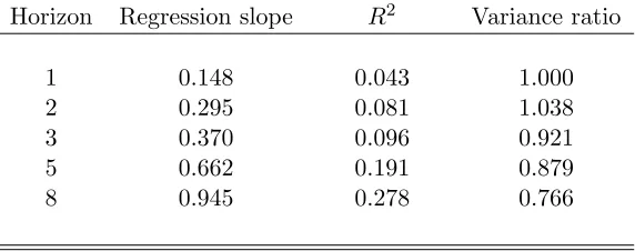
in Panel A of Table 1.8 In addition, the volatility of equity premium is 19.02 percent. These values are hard to match in a standard asset-pricing model under reasonable calibration. This fact is often referred to as the equity premium, riskfree rate and equity volatility puzzles (see Campbell (1999) for a survey). Panel B of Table 1 reports that the log dividend yield predicts long-horizon realized excess returns. It also shows that the regression slopes andR2’s increase
with the return horizon. This return predictability puzzle is first documented by Campbell
and Shiller (1988b) and Fama and French (1988a). Panel B of Table 1 also reports variance
7
The Fortran codes and a technical appendix detailing our numerical method are available upon request.
8
ratio statistics for the equity premium. These ratios are generally less than 1 and fall with the horizon. This evidence suggests that excess returns are negatively serially correlated, or asset prices are mean reverting (Fama and French (1988b) and Poterba and Summers (1988)).
[Insert Table 1 Here.]
In addition to the preceding puzzles, we will use our model to explain three other stylized facts: (i) procyclical variation in price-dividend ratios (Campbell and Shiller (1988a)), (ii) countercyclical variation in conditional expected equity premia (Campbell and Shiller (1988a,b)
and Fama and French (1989)), and (iii) persistent and countercyclical variation in conditional volatility of equity premium (Bollerslev et al. (1992)).
To explain the above asset pricing phenomena, we calibrate our model at the annual fre-quency. We first calibrate parameters in consumption and dividends processes. Cecchetti et al. (2000) apply Hamilton’s maximum likelihood method to estimate parameters in (13) using the annual per capita US consumption data covering the period 1890-1994. Table 2 reproduces their estimates. This table reveals that the high-growth state is highly persistent, with consumption
growth in this state being 2.251 percent. The economy spends most of the time in this state with the unconditional probability of being in this state given by (1−λ22)/(2−λ11−λ22) = 0.96.
The low-growth state is moderately persistent, but very bad, with consumption growth in this state being−6.785 percent. The long-run average rate of consumption growth is 1.86 percent.
[Insert Table 2 Here.]
We next calibrate parameters in the dividend process (14). We follow Abel (1999) and set the leverage parameterφ= 2.74.We then follow Bansal and Yaron (2004) and choosegd=−0.0323
so that the average rate of dividend growth is equal to that of consumption growth. We choose
σd to match the volatility of dividend growth in the data. Using different century-long annual
samples, this volatility is equal to 0.136 and 0.142, according to the estimates given by Cecchetti et al. (1990) and Campbell (1999), respectively. Here, we take 0.13 and findσd= 0.084. Our
calibrated values of σd and φ imply that the correlation between consumption growth and
dividend growth is about 0.76. This value may seem high. However, Campbell and Cochrane (1999) argue that the correlation is difficult to measure and it may approach 1.0 in the very long run since dividends and consumption should share the same long-run trends.
Now, we select baseline preference parameters. We follow Bansal and Yaron (2004) and set EIS to 1.5, implyingρ= 1/1.5.An EIS greater than 1 is critical to generate procyclical variation
the main force of our model comes from ambiguity aversion, but not risk aversion. We next select the discount factor β and ambiguity aversion parameter η to match the mean riskfree rate of 0.0266 and the mean equity premium of 0.0575 from the data reported in Table 1. We
find β= 0.975 and η= 8.864.
There is no independent study of the magnitude of ambiguity aversion in the literature. To judge whether our calibrated value is reasonable, we conduct a thought experiment related to the Ellsberg Paradox (Ellsberg (1961)) in a static setting. Suppose there are two urns. Subjects are told that there are 50 black and 50 white balls in urn 1. Urn 2 also contains 100 balls, but may contain either 100 black balls or 100 white balls. If a subject picks a black ball from an urn, he wins a prize, otherwise he does not win or lose anything. Experimental evidence
reveals that most subjects prefer to bet on urn 1 rather than urn 2 (Camerer (1999) and Halevy (2007)). Paradoxically, if the subject is asked to pick a white ball, he still prefers to bet on urn 1. The standard expected utility model with any beliefs or any risk aversion level cannot explain this paradox. Our adopted smooth ambiguity model in the static setting (1) can explain this paradox whenever subjects display ambiguity aversion (i.e., v is more concave than u).Thus, ambiguity aversion and risk aversion have distinct behavioral meanings.
Formally, Let w be a subject’s wealth level anddbe the prize money. Because the subject knows that the distribution of black and white balls in urn 1 is (1/2,1/2), when he evaluates a bet on urn 1, his utility level in terms of certainty equivalent is equal to:
u−1
µ 1
2u(w+d) + 1 2u(w)
¶
. (21)
The subject believes that there are two possible equally likely distributions (0,1) and (1,0) in urn 2, and thus Π = {(0,1),(1,0)} and µ = (1/2,1/2). But he is not sure which one is the true distribution and is averse to this uncertainty. When he evaluates a bet on urn 2, his utility level in terms of certainty equivalent is equal to:
v−1
µZ
Π
v
µ
u−1
µZ
S
u(c)dπ
¶¶
dµ(π) ¶
, (22)
wherec=w+dorwandS={black, white}.The expression in (21) is larger than that in (22) if
vis more concave thanu,causing the subject to bet on urn 1 rather than urn 2. The difference
between the certainty equivalents in (21) and (22) is a measure of ambiguity premium. Given power functions of u and v and fixing the risk aversion parameter, we can use the size of the ambiguity premium to gauge the magnitude of ambiguity aversion.9 It is straightforward to compute that the ambiguity premium is equal to 1.7 percent of the expected prize value for our
9See Chen, Ju and Miao (2009) for a more extensive discussion and an application of our generalized recursive
calibrated ambiguity aversion parameter η = 8.864, when we set γ = 2 and the prize-wealth ratio of 1 percent. Increasing the prize-wealth ratio raises the ambiguity premium. Camerer (1999) reports that the ambiguity premium is typically in the order of 10-20 percent of the
expected value of a bet in the Ellsberg-Paradox type experiments. Given this evidence, our calibrated ambiguity aversion parameter seems small and reasonable.
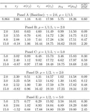
4.2. Unconditional Moments of Returns
As a first check of the performance of our calibrated model, we compare the model prediction of the volatility of the equity premium and the volatility of the riskfree rate with the data. Panel
A of Table 3 reports model results. This table reveals that our model can match the volatility of the equity premium in the data quite closely (0.1826 versus 0.1902). However, our model generated volatility of the riskfree rate is lower than the data (0.0116 versus 0.0513). Campbell (1999) argues that the high volatility of the riskfree rate in the century-long annual data could be due to large swings in inflation in the interwar period, particularly in 1919-21. Much of this volatility is probably due to unanticipated inflation and does not reflect the volatility in the ex ante real interest rate. Campbell (1999) reports that the annualized volatility of the real return
on Treasury Bills is 1.8 percent using the US postwar quarterly data.
[Insert Table 3 Here.]
To understand why our model is successful in matching unconditional moments of returns, we conduct a comparative statics analysis in Panels B-E of Table 3. The first row of each of these panels gives the result of benchmark model II with Epstein-Zin preferences under Bayesian learning. We first consider the effects of the three standard parameters (β, ρ, γ) familiar from the Epstein-Zin model. Equation (17) implies that the riskfree rateRf,t+1 = 1/Et£Mzt+1,t+1
¤
.
Because the pricing kernel Mzt+1,t+1 increases with the subjective discount factor β, a high
value of β helps match the low riskfree rate. Table 3 reveals that an increase in EIS (or 1/ρ) from 1.5 to 2.0 generally lowers the riskfree rate and stock returns due to the high intertemporal substitution effect. In addition, an increase inγ from 2.0 to 5.0 also lowers the riskfree rate and raises stock returns. These results follow from the usual intuition in the Epstein-Zin model.
Next, consider the role of ambiguity aversion, which is unique in our model. Table 3 reveals that an increase in the ambiguity aversion parameterη lowers the riskfree rate and raises stock
returns. The intuition follows from the discussion in Section 3.2. An ambiguity averse agent displays pessimistic behavior by attaching more weight to the worst state with low continuation utilities. Thus, he saves more for the future and invests less in the stock. In addition, as more weight is attached to the low-growth state, there is less variation of Et
£
Mzt+1,t+1
¤
the riskfree rateRf,t+1is less volatile. By contrast, ambiguity aversion makes the pricing kernel
Mzt+1,t+1 more volatile as revealed by the last term in (16), leading to high and volatile equity
premium. It also generates a high market price of uncertainty defined by the ratio of the
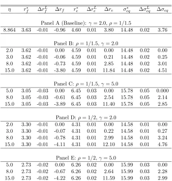
volatility of the pricing kernel and the mean of the pricing kernel (Hansen and Jagannathan (1991)). For our calibrated baseline parameter values, the market price of uncertainty is equal to 0.60, as reported in Panel A Table 3. It is equal to 0.09 in benchmark model II with η=γ. Finally, we analyze the role of learning under ambiguity. We decompose the riskfree rf in
our model into three components:
rf =rf∗+
¡
rfL−r∗f¢ +¡
rf −rLf
¢
, (23)
where r∗
f, rfL, and rf are the means of the riskfree rate delivered by benchmark model I,
benchmark model II, and our ambiguity model, respectively. We do a similar decomposition for the mean stock returns and the volatility of the equity premium.10 Table 4 presents this decomposition.
[Insert Table 4 Here.]
Panel A of this table shows that under the baseline parameter values, benchmark model I with full information predicts that the mean riskfree rater∗
f = 0.0363,the mean equity returns
r∗
e = 0.046, and the volatility of equity premium σeq∗ = 0.1448.For benchmark model II with
Epstein-Zin preferences, the standard Bayesian learning lowers the riskfree rate and raises the
equity return and equity volatility, but by a negligible amount. By contrast, the component (rf−rfL) due to learning under ambiguity accounts for most of the decrease in the riskfree rate
and the increase in the equity return and the volatility of the equity premium. In addition, the magnitude of this component is larger for a larger degree of ambiguity aversion. We find the same result also for various values of the risk aversion parameter as presented in Panels B-C. In particular, when the risk aversion parameterγ = 2 and 5,the corresponding effects of Bayesian
learning are to lower the mean riskfree rate by 0.01 and 0.03 percent, to raise the mean stock return by 0.01 and 0.03 percent, and to raise the equity premium volatility by 0.02 and 0.05 percent. These effects are quantitatively negligible. Increasing EIS from 1.5 to 2.0 does not change this result much as revealed by Panels D-E.
A surprising feature of benchmark model II with Bayesian learning is that equity premium can become negative when risk aversionγis sufficiently large in the special case of time-additive utility γ = ρ. Increasing risk aversion may worsen the equity premium puzzle. In a similar
10In a continuous-time multiple-priors model without learning, Chen and Epstein (2002) provide a similar
continuous-time model, Veronesi (2000) proves this result analytically. The intuition is that an increase in risk aversion raises the agent’s hedging demand for the stock after bad news in dividends, thereby counterbalancing the negative pressure on prices due to the bad news in
dividends. The former effect may dominate so that the pricing kernel and stock returns are positively correlated, resulting in negative equity premia (see equation (19)). By contrast, in our model, an ambiguity averse agent invests less in the stock, thereby counterbalancing the preceding hedging effect. In contrast to risk aversion, an increase in the degree of ambiguity aversion helps increase equity premium.
4.3. Price-Consumption and Price-Dividend Ratios
Panel A of Figure 1 presents the price-consumption ratio as a function of the posterior proba-bilities µt of the high-growth state for three values ofη, holding other parameters fixed at the
baseline values. It reveals two properties. First, the price-consumption ratio is increasing and convex. The intuition is similar to that described by Veronesi (1999) who analyzes time-additive expected exponential utility. When times are good (µt is close to 1), a bad piece of news
de-creases µt,and hence decreases future expected consumption. But it also increases the agent’s
uncertainty about consumption growth sinceµt is now closer to 0.5,which gives approximately
the maximal conditional volatility of the posterior probability of the high-growth state in the next period. Since the agent wants to be compensated for bearing more risk, they will require an additional discount on the price of consumption claims. Thus, the price reduction due to a bad piece of news in good times is higher than the reduction in expected future consumption. By contrast, suppose the agent believes times are bad and hence µt is close to zero. A good
piece of news increases the expected future consumption, but also raises the agent’s perceived uncertainty since it moves µt closer to 0.5. Thus, the price-consumption ratio increases, but
not as much as it would in a present-value model.
The second property of Panel A of Figure 1 is that an increase in the degree of ambiguity aversion lowers the price-consumption ratio because it induces the agent to invest less in the asset. In addition, an increase in the degree of ambiguity aversion raises the curvature of the price-consumption ratio function, thereby helping increase the asset price volatility. In the
special case of benchmark model II with η = γ, the price-consumption ratio is close to be a linear function of the state beliefs.11 Thus, this model cannot generate high asset price volatility.
[Insert Figure 1 Here]
11
Panel B of Figure 1 presents the price-consumption ratio function for various values of ρ, holding other parameters fixed at the baseline values. It reveals that the price-consumption ratio is an increasing function ofµt when ρ <1, while it is a decreasing function when ρ >1.
When ρ = 1, it is equal to β/(1−β) by (18) because wealth is equal to consumption plus the price of consumption claims. This result follows from the usual intuition in the Epstein-Zin model (see Bansal and Yaron (2004)). When ρ < 1,EIS is greater than 1 and hence the intertemporal substitution effect dominates the wealth effect. In response to good news of consumption growth, the agent buys more assets and hence the price-consumption ratio rises. The opposite result holds true whenρ >1.
Panels C and D of Figure 1 present similar figures for the price-dividend ratio. We find that
the effects ofηand ρare similar. One difference is that the price-dividend ratio is not constant when ρ= 1 because dividends and aggregate consumption are not identical in our model. Due to leverage, we need a sufficiently small EIS (or a large ρ) to make the price-dividend ratio decrease withµt.Bansal and Yaron (2004) find a similar result in a full information model with
Epstein-Zin preferences.
In summary, ambiguity aversion helps generate the variation in the price-consumption and
dividend ratios. An EIS greater than 1 is important for generating procyclical price-consumption and price-dividend ratios.
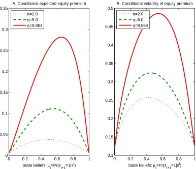
4.4. Time-Varying Equity Premia and Equity Volatility
Panels A of Figure 2 plots the conditional expected equity premium as a function of the posterior probability µt of the high-growth state for various values of η. We find that this function is
hump-shaped and peaks when µt is around 0.6. This shape seems to suggest that a negative
consumption shock can lead to either higher or lower equity premium, depending on whether
µt is close to 0 or to 1. However, since the economy spends most of the time in the
high-growth state, the steady-state distribution of the posterior is highly skewed. This implies that
µt is close to 1 in most of the time, leading to the pattern that equity premium rises following
negative consumption shocks. As a result, our model can generate the countercyclical variation in equity premium observed in the data.
[Insert Figure 2 Here.]
Panel B of Figure 2 plots the conditional volatility of equity premium as a function of µt
for various values of η. This function is also hump-shaped, with the maximum attained at
a value of µt close to 0.6. Following similar intuition discussed above, our model generates
countercyclical variation in conditional volatility of equity premium observed in the data. In addition, ambiguity aversion helps amplify this variation.
Our model can also generate persistent changes in conditional volatility of equity premium, documented by Bollerslev et al. (1992). The intuition is that the agent’s beliefs are persistent in the sense that if he believes the high-growth state today has a high probability, then he expects the high-growth state tomorrow also has a high probability on average. The persistence of
beliefs drives the persistence of the volatility of equity premium.
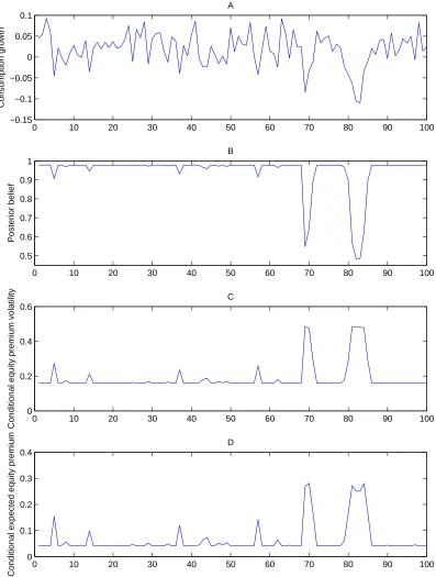
[Insert Figure 3 Here.]
Figure 3 illustrates the time-varying properties of the expected equity premium and the volatility of equity premium by a Monte Carlo simulation. Panel A plots a time series of con-sumption growth simulated using (13). Panel B plots the time series of the posterior probability of the high-growth stateµt,computed using (15). It reveals that in most of the time the agent
believes that the economy is in the high-growth state in that µt is close to 1. After a few
negative shocks to consumption growth, the agent believes the low-growth state is more likely in that µt decreases and is close to 0.5. At this value, the agent’s perceived uncertainty about
the high-growth state in the next period is the highest. Using the simulated series of con-sumption growth, dividend growth, and the posterior probabilities, we can compute the series of conditional volatility of stock returns and conditional expected equity premium. We plot these series in Panels C and D of Figure 3, respectively. From these panels, we can see that both the conditional volatility of equity premium and conditional expected equity premium are
time-varying and move with business cycles countercyclically.
4.5. Serial Correlation and Predictability of Returns
To examine the ability of our model to generate the serial correlation and predictability of returns reported in Table 2, we compare our model with benchmark models I and II. Table 5 reports the model implied values of the variance ratios, the regression slopes and theR2’s, at
From Table 5, we observe that all three models can generate the pattern that variance ratios are less than 1 and decrease with the horizon, suggesting that excess returns are negatively serially correlated. In terms of predictive regressions, benchmark models I and II deliver very
smallR2’s, implying weak predictability.12 One may expect that learning should help generate return predictability. The intuition is that the change of state beliefs is persistent, and hence the price-dividend ratio is also persistent and positively serially correlated. However, Table 5 reports that benchmark model II with Bayesian learning helps little quantitatively. In a related model, Brandt et al. (2004) find a similar result.
We finally consider our model in which we introduce ambiguity aversion into benchmark model II. Table 5 reveals that while all three models can generate the pattern that the regression
slopes increase with the horizon, our model with learning under ambiguity produces much more significant quantitative effects. In particular, compared to benchmark models I and II, our model implied values of the regression slopes and R2’s are much higher. However, our model still cannot replicate the same numbers estimated from the data reported in Panel B of Table 2. In addition, all three models cannot generate the pattern thatR2’s increase with the horizon.
The model predictedR2’s first increase with the horizon and then decrease with it after period 3.
This could be due to the fact that the model generated price-dividend ratios are not persistent enough.13 We should recognize that the predictability results in the empirical literature are quite sensitive to data sets, changing samples, and estimation techniques (Welch and Goyal (2008)). Thus, one should be cautious in interpreting empirical evidence on predictability.
[Insert Table 5 Here]
5.
Conclusion
In this paper, we have proposed a novel generalized recursive smooth ambiguity model which allows a three-way separation among risk aversion, ambiguity aversion and intertemporal sub-stitution. This model nests some utility models commonly adopted in the literature as special cases. We also propose a tractable homothetic specification and apply this model to asset
pric-ing. When modelling consumption growth and dividend growth as regime-switching processes (nonlinear counterpart of the long-run risk processes as in Bansal and Yaron (2004)), our asset pricing model can help explain a variety of asset pricing puzzles. Our calibrated model can match the mean equity premium, the mean riskfree rate, and the volatility of equity premium
12
Beeler and Campbell (2009) and Garcia et al. (2008) re-examine the Bansal-Yaron model and find that it cannot match the predictability in the data, contrary to the finding of Bansal and Yaron (2004).
13
observed in the data. In addition, our model can generate a variety of dynamic asset pric-ing phenomena, includpric-ing the procyclical variation of price-dividend ratios, the countercyclical variation of equity premia and equity volatility, and the mean reversion of excess returns.
We show that ambiguity aversion and learning under ambiguity play a key role in explain-ing asset pricexplain-ing puzzles. An ambiguity averse agent displays pessimistic behavior in that he attaches more weight to the pricing kernel in bad times when his continuation values are low. This pessimistic behavior helps propagate and amplify shocks to consumption growth, and gen-erates time-varying equity premium. We also find that Bayesian learning in the expected utility framework has a modest quantitative effect on asset returns, while learning under ambiguity is important to explain dynamic asset pricing phenomena. One limitation of our model is that it
cannot reproduce the predictability pattern in the data.
Other models can also simultaneously generate the unconditional moments and dynamics of asset returns observed in the data. For example, Campbell and Cochrane (1999) introduce a slow moving habit or time-varying subsistence level into a standard power utility function.14 As a result, the agent’s risk aversion is time varying. Bansal and Yaron (2004) apply the Epstein-Zin preferences, and incorporate fluctuating volatility and a persistent component in
consumption growth.15 Their calibrated risk aversion parameter is 10. Our model of con-sumption and dividend processes is similar to Bansal and Yaron (2004), but is much easier to estimate. We shut down exogenous fluctuations in consumption growth volatility and analyze how endogenous learning under ambiguity can generate time-varying equity premium.
We view our model as a first step toward understanding the quantitative implications of learning under ambiguity for asset returns. We have shown that our model can go a long way to explain many asset pricing puzzles. Much work still remains to be done. For example,
how to empirically estimate parameters of ambiguity aversion, risk aversion, and intertempo-ral substitution would be important future research topics. In addition, our proposed novel generalized recursive ambiguity model can be applied to many other problems in finance and macroeconomics.
14
Ljungqvist and Uhlig (2009) show that government interventions that occasionally destroy part of endowment can be welfare improving when endogenizing aggregate consumption choices in the Campbell-Cochrane habit formation model.
15
Appendix
A
Proofs of Results in Section 3.2
We follow the method of Hansen et al. (2008) to derive the marginal utility of consumption and continuation value as:
M Ct=
∂Vt(C)
∂Ct
= (1−β)VtρCt−ρ,
M Vzt+1,t+1=
∂Vt(C)
∂Vzt+1,t+1
=βVtρ[Rt(Vt+1)]η−ρ
³ Ezt+1,t
h
Vt1+1−γi´−
η−γ 1−γ
Vt−+1γ,
where Vzt+1,t+1 denotes the continuation value Vt+1(C) conditioned on the period t+ 1 state
being zt+1. The pricing kernel is given by Mzt+1,t+1 =
¡
M Vzt+1,t+1
¢
(M Ct+1)/M Ct, which
delivers (16).
We next use the dynamic programming method of Epstein and Zin (1989) to derive other results in Section 3.2. Suppose the agent trades N assets. The budget constraint is Wt+1 =
(Wt−Ct)Rw,t+1,where the return on the wealth portfolio Rw,t+1 is equal to PNk=1ψktRk,t+1,
ψktis the portfolio weight on assetk,andRk,t+1denotes its return. The value functionJ(Wt, µt)
satisfies the Bellman equation:
J(Wt, µt) = max
·
(1−β)Ct1−ρ+β
½µ
µt
¡ E1,t
£
J1−γ(Wt+1, µt+1)
¤¢11−η−γ
(A.1)
+ (1−µt)
¡ E2,t
£
J1−γ(Wt+1, µt+1)
¤¢11−η−γ
¶¾11−η−ρ#
1 1−ρ
.
Conjecture
J(Wt, µt) =AtWt, andCt=atWt, (A.2)
whereAtandatare to be determined. Substituting (A.2) and the budget constraint into (A.1),
we can then rewrite the Bellman equation as:
At= max at,{ψkt}
(1−β)a1t−ρ+ (1−at)1−ρβ
µ Eµt
³ Ezt+1,t
h
(At+1Rw,t+1)1−γ
i´11−η
−γ ¶ 1−ρ 1−η 1 1−ρ
Use the first-order condition for consumption to derive:
µ
at
1−at
¶−ρ = β
1−β
µ Eµt
³ Ezt+1,t
h
(At+1Rw,t+1)1−γ
i´11−η
−γ
¶
1−ρ 1−η
. (A.3)
From the above two equations, we have:
At= (1−β)1/(1−ρ)at−ρ/(1−ρ)= (1−β)1/(1−ρ)
µ
Ct
Wt
¶−ρ/(1−ρ)
. (A.4)
References
Abel, Andrew B., 1999, Risk Premia and Term Premia in General Equilibrium, Journal of Monetary Economics 43, 3-33.
Abel, Andrew B., 2002, An Exploration of the Effects of Pessimism and Doubt on Asset Returns, Journal of Economic Dynamics and Control 26, 1075-1092.
Anderson, Evan W., Lars Peter Hansen, and Thomas J. Sargent, 2003, A Quartet of Semi-groups for Model Specification, Robustness, Prices of Risk, and Model Detection,Journal of the European Economic Association,1, 68-123.
Backus, David, Bryan Routledge, and Stanley Zin, 2005, Exotic Preferences for Macroe-conomists, in Mark Gertler and Kenneth Rogoff (Eds.), NBER Macroeconomics Annual 2004, 319-390. Cambridge: MIT Press.
Bansal, Ravi and Amir Yaron, 2004, Risks for the Long Run: A Potential Resolution of Asset Pricing Puzzles, Journal of Finance 59, 1481-1509.
Beeler, Jason and John Y. Campbell, 2009, The Long-Run Risks Model and Aggregate Asset Prices: An Empirical Assessment, working paper, Harvard University.
Bollerslev, Tim, Ray Y. Chou, and Kenneth F. Kroner, 1992, ARCH Modelling in Finance: A Review of the Theory and Empirical Evidence,Journal of Econometrics 52, 5-59.
Brandt, Michael W., Qi Zeng, and Lu Zhang, 2004, Equilibrium Stock Return Dynamics under Alternative Rules of Learning about Hidden States,Journal of Economic Dynamics and Control 28, 1925-1954.
Brennan, Michael J. and Yihong Xia, 2001, Stock Price Volatility and the Equity Premium,
Journal of Monetary Economics 47, 249-283.
Cagetti, Marco, Lars Peter Hansen, Thomas Sargent, and Noah Williams, 2002, Robustness and Pricing with Uncertain Growth,Review of Financial Studies 15, 363-404.
Camerer, Colin F., 1999, Ambiguity-Aversion and Non-Additive Probability: Experimental Evidence, Models and Applications, Uncertain Decisions: Bridging Theory and Experi-ments, ed. by L. Luini, pp. 53-80. Kluwer Academic Publishers.
Campbell, John Y., 1999, Asset Prices, Consumption and the Business Cycle, in John B. Tay-lor, and Michael Woodford, eds.: Handbook of Macroeconomics, vol. 1 (Elsevier Science, North-Holland, Amsterdam).
Campbell, John Y., and John H. Cochrane, 1999, By Force of Habit: A Consumption-Based Explanation of Aggregate Stock Market Behavior, Journal of Political Economy 107, 205-251.
Campbell, John Y. and Robert J. Shiller, 1988a, The Dividend-Price Ratio and Expectations of Future Dividends and Discount Factors,Review of Financial Studies 1, 195-227.
Campbell, John Y. and Robert J. Shiller, 1988b, Stock Prices, Earnings, and Expected Divi-dends,Journal of Finance 43, 661-676.
Cao Henry, Tan Wang, and Harold Zhang, 2005, Model Uncertainty, Limited Market Partici-pation, and Asset Prices, Review of Financial Studies 18, 1219-1251.
Cecchetti, Stephen G., Pok-sang Lam, and Nelson C. Mark, 1990, Mean Reversion in Equilib-rium Asset Prices,American Economic Review 80, 398-418.
Cecchetti, Stephen G., Pok-sang Lam, and Nelson C. Mark, 1993, The Equity Premium and the Riskfree Rate: Matching the Moments,Journal of Monetary Economics, 31, 21-45.
Cecchetti, Stephen G., Pok-sang Lam, and Nelson C. Mark, 2000, Asset Pricing with Distorted Beliefs: Are Equity Returns Too Good to Be True, American Economic Review 90, 787-805.
Chen, Hui, Nengjiu Ju, and Jianjun Miao, 2009, Dynamic Asset Allocation with Ambiguous Return Predictability, working paper, Boston University.
Chen, Zengjin and Larry G. Epstein, 2002, Ambiguity, Risk and Asset Returns in Continuous Time,Econometrica 4, 1403-1445.
Collard, Fabrice, Sujoy Mukerji, Kevin Sheppard, and Jean-Marc Tallon, 2009, Ambiguity and Historical Equity Premium, working paper, Oxford University.
David, Alexander, 1997, Fluctuating Confidence in Stock Markets: Implications for Returns and Volatility, Journal of Financial and Quantitative Analysis 32, 427-462.
Detemple, Jerome, 1986, Asset Pricing in a Production Economy with Incomplete Information,
Journal of Finance 41, 383-391.
Dothan, Michael U. and David Feldman, 1986, Equilibrium Interest Rates and Multiperiod Bonds in a Partially Observable Economy, Journal of Finance 41, 369-382.
Duffie, Darrell and Costis Skiadas, 1994, Continuous-Time Security Pricing: A Utility Gradi-ent Approach, Journal of Mathematical Economics 23, 107-132.
Ellsberg, Daniel, 1961, Risk, Ambiguity and the Savage Axiom, Quarterly Journal of Eco-nomics 75, 643-669.
Epstein, Larry G. , 1999, A Definition of Uncertainty Aversion, Review of Economic Studies
66, 579-608.
Epstein, Larry G. and Jianjun Miao, 2003, A Two-Person Dynamic Equilibrium under Ambi-guity,Journal of Economic Dynamics and Control 27, 1253-1288.
Epstein, Larry G. and Martin Schneider, 2007, Learning under ambiguity,Review of Economic Studies 74, 1275-1303.
Epstein, Larry G. and Martin Schneider, 2008, Ambiguity, Information Quality and Asset Pricing,Journal of Finance 63, 197-228.
Epstein, Larry G. and Tan Wang, 1994, Intertemporal Asset Pricing under Knightian Uncer-tainty, Econometrica 62, 283-322.
Epstein, Larry G. and Stanley Zin, 1989, Substitution, Risk Aversion and the Temporal Be-havior of Consumption and Asset Returns: A Theoretical Framework,Econometrica 57, 937-969.
Epstein, Larry G. and Stanley Zin, 1991, Substitution, Risk Aversion and the Temporal Be-havior of Consumption and Asset Returns: An Empirical Analysis, Journal of Political Economy 99, 263-286.
Ergin, Huluk I. and Faruk Gul, 2009, A Theory of Subjective Compound Lotteries, Journal of Economic Theory 144, 899-929.
Fama, Eugene F., and Kenneth R. French, 1988a, Dividend Yields and Expected Stock Re-turns,Journal of Financial Economics 22, 3-25.
Fama, Eugene F. and Kenneth R. French, 1988b, Permanent and Temporary Components of Stock Prices,Journal of Political Economy 96, 246-273.
Fama, Eugene F. and Kenneth R. French, 1989, Business Conditions and Expected Returns on Stocks and Bonds,Journal of Financial Economics 25, 23-49.
Garcia, Rene, Nour Meddahi, and Romeo Tedongap, 2008, An Analytical Framework for Assessing Asset Pricing Models and Predictability, working paper, Edhec Business School.
Garlappi, Lorenzo, Raman Uppal, and Tan Wang, 2007, Portfolio Selection with Parameter and Model Uncertainty: A Multi-Prior Approach,Review of Financial Studies 20, 41-81.
Ghirardato, Paolo and Massimo Marinacci, 2002, Ambiguity Made Precise: A Comparative Foundation,Journal of Economic Theory 102, 251-289.
Gilboa, Itzach and David Schmeidler, 1989, Maxmin Expected Utility with Non-unique Priors,
Journal of Mathematical Economics 18, 141-153.
Gollier, Christian, 2006, Does Ambiguity Aversion Reinforce Risk Aversion? Applications to Portfolio Choices and Asset Prices, working paper, University of Toulouse.
Halevy, Yoran, 2007, Ellsberg Revisited: An Experimental Study, Econometrica 75, 503-536.
Hamilton, James D., 1989, A New Approach to the Economic Analysis of Nonstationary Time Series and the Business Cycle,Econometrica 57, 357-384.
Hansen, Lars Peter and Ravi Jagannathan, 1991, Implications of security market data for models of dynamic economies,Journal of Political Economy 99, 225-262.
Hansen, Lars Peter, John C. Heaton, and Nan Li, 2008, Consumption Strikes Back?: Measur-ing Long-Run Risk, Journal of Political Economy 116, 260-302.
Hansen, Lars Peter and Thomas J. Sargent, 2001, Robust Control and Model Uncertainty,
American Economic Review 91, 60-66.
Hansen, Lars Peter and Thomas J. Sargent, 2007a, Recursive Robust Estimation and Control without Commitment,Journal of Economic Theory 136, 1-27.
Hansen, Lars Peter and Thomas J. Sargent, 2007b, Fragile Beliefs and the Price of Model Uncertainty, working paper, New York University.
Hansen, Lars Peter and Thomas J. Sargent, 2008, Robustness, Princeton University Press, Princeton and Oxford.
Hansen, Lars Peter, Thomas J. Sargent, and Thomas Tallarini, 1999, Robust Permanent Income and Pricing, Review of Economic Studies 66, 873-907.
Hayashi, Takashi and Jianjun Miao, 2009, Generalized Recursive Ambiguity Preferences, work in progress, Boston University.
Ju, Nengjiu and Jianjun Miao, 2007, Ambiguity, Learning, and Asset Returns, working paper, Boston University.
Judd, Kenneth, 1998, Numerical Methods in Economics, MIT Press, Cambridge, MA.
Kandel, Shmuel and Robert F. Stambaugh, 1991, Asset Returns and Intertemporal Prefer-ences,Journal of Monetary Economics 27, 39–71.
Keynes, Maynard, 1936, The General Theory of Employment, Interest, and Money, London Macmillan.
Klibanoff, Peter, Massimo Marinacci, and Sujoy Mukerji, 2005, A Smooth Model of Decision Making under Ambiguity,Econometrica 73, 1849-1892.
Klibanoff, Peter, Massimo Marinacci, and Sujoy Mukerji, 2008, Recursive Smooth Ambiguity Preferences, forthcoming inJournal of Economic Theory.
Knight, Frank, 1921,Risk, Uncertainty, and Profit, Boston: Houghton Mifflin.
Kreps, David, M. and Evan L. Porteus, 1978, Temporal Resolution of Uncertainty and Dy-namic Choice,Econometrica 46, 185-200.
Leippold, Markus, Fabio Trojani, and Paolo Vanini, 2008, Learning and Asset Prices under Ambiguous Information,Review of Financial Studies 21, 2565-2597.
Ljunqvist, Lars and Harold Uhlig, 2009, Optimal Endowment Destruction under Campbell-Cochrane Habit Formation, NBER working paper #14772.
Lucas, Robert E., 1978, Asset Prices in an Exchange Economy, Econometrica 46, 1429-1445.
Maccheroni, Fabio, Massimo Marinacci, and Aldo Rustichini, 2006, Ambiguity Aversion, Ro-bustness and the Variational Representation of Preferences,Econometrica 74, 1447-1498.
Maenhout, Pascal J., 2004, Robust Portfolio Rules and Asset Pricing, Review of Financial Studies 17, 951-983.
Mehra, Rajnish and Edward C. Prescott, 1985, The Equity Premium: A Puzzle, Journal of Monetary Economics 15, 145-161.
Nau, Robert F., 2006, Uncertainty Aversion with Second-Order Utilities and Probabilities,
Management Science 52, 136-145.
Poterba, James M. and Lawrence H. Summers, 1988, Mean Reversion in Stock Prices: Evi-dence and Implications,Journal of Financial Economics 22, 27-59.
Routledge, Bryan and Stanley Zin, 2001, Model Uncertainty and Liquidity, NBER working paper #8683.
Segal, Uzi, 1987, The Ellsberg Paradox and Risk Aversion: An Anticipated Utility Approach,
International Economic Review 28, 175-202.
Seo, Kyounwon, 2008, Ambiguity and Second-Order Belief, forthcoming inEconometrica.
Shiller, Robert J., 1981, Do Stock Prices Move too Much to be Justified by Subsequent Changes in Dividends? American Economic Review 71, 421-436.
Tallarini, Thomas D. Jr., 2000, Risk-Sensitive Real Business Cycles, Journal of Monetary Economics 45, 507-532.
Uppal, Raman and Tan Wang, 2003, Model Misspecification and Underdiversification,Journal of Finance 58, 2465-2486.
Veronesi, Pietra, 1999, Stock Market Overreaction to Bad News in Good Times: A Rational Expectations Equilibrium Model, Review of Financial Studies 12, 975-1007.
Veronesi, Pietro, 2000, How Does Information Quality Affect Stock Returns? Journal of Finance 55, 807-839.
Weil, Philippe, 1989, The Equity Premium Puzzle and the Risk-Free Rate Puzzle,Journal of Monetary Economics 24, 401-421.
Weitzman, Martin L., 2007, Subjective Expectations and Asset-Return Puzzles, American Economic Review 97, 1102-1130.